Adaptive AM–FM Signal Decomposition With Application to ... - ICS

296 IEEE TRANSACTIONS ON AUDIO, SPEECH, AND LANGUAGE PROCESSING, VOL. 19, NO. 2, FEBRUARY 2011
last step of aQHM, the signal can be finally approximated as
the sum of its AM–FM components
(28)
Therefore, aQHM suggests an algorithm for the adaptive
AM–FM decomposition of a signal.
For applications such as speech analysis for the purpose of
voice function assessment (i.e., voice disorders, analysis of
tremor), and voice modification, the one sample time step is
accepted. In other applications however, such as speech synthesis,
larger steps are required. In this case, the instantaneous
values of frequency, amplitude, and phase should be estimated
from the set of parameters computed at every analysis time
instant . In SM, between two consecutive synthesis instants,
linear interpolation for the amplitudes and cubic interpolation
for phases were suggested [24]. In aQHM, many analysis time
instants can be considered under the analysis window. For
instantaneous amplitude estimation, we used splines, although
other choices, such as linear interpolation, are possible. Such a
simple solution is not, however, possible for the estimation of
instantaneous phase. For this purpose, we will now describe a
nonparametric approach as an alternative to the cubic interpolation
method suggested in [24].
Based on the definition of phase, the instantaneous phase for
the th component can be computed as the integral of the computed
instantaneous frequency. For instance, between two consecutive
analysis time instants and , the instantaneous
phase can be computed as
(29)
This solution however does not take into account the frame
boundary conditions at , which means that there is no guarantee
that , where is the closet integer
to
. We suggest modifying (29) in
order to guarantee phase continuation over frame boundaries as
follows:
(30)
Note that the derivative of the instantaneous phase over time in
both formulas provide the instantaneous frequency computed
from to . In (30), the continuation of instantaneous frequency
at the frame boundaries is also guaranteed by the use of
the sine function (although other choices may be used as well).
Moreover, it can be easily shown that using (30) the instantaneous
phase at will be equal to if is selected
to be
(31)
where is computed as before.
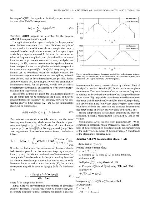
In Fig. 4, the two above formulas are compared on a synthetic
example. The signal was analyzed frame-by-frame using QHM
to compute the phase values at the frame boundaries. The actual
Fig. 4. Actual instantaneous frequency (dashed line) and estimated instantaneous
frequency (solid line) as the derivative of the instantaneous phase computed
from (29) (upper panel) and (30) (lower panel).
instantaneous frequency contour (shown by a dashed line) of
the signal is used in (29) and in (30) for the instantaneous phase
computation. Then an estimation of the instantaneous frequency
is obtained as the derivative over time of the computed instantaneous
phases. Fig. 4(a) and (b) show the estimated instantaneous
frequency (solid line) when (29) and (30) are used, respectively.
It is obvious that in the former case there are spikes at the frame
boundaries while in the latter case, the estimated instantaneous
frequency is free of artefact and very close to the actual one.
Having computing the instantaneous amplitude and phase information,
the signal reconstruction is obtained by (28), as previously.
Summarizing, aQHM suggests a non-parametric AM–FM decomposition
algorithm which proceeds by successive adaptations
of the decomposition basis functions to the characteristics
of the underlying sine waves of the input signal. A pseudocode
of the algorithm is presented next.
Adaptive AM–FM decomposition alg. (aQHM)
1) Initialization (QHM):
Provide initial estimate
For
a) Compute , using as initial frequency
estimates in (2)
b) Update using (26a) and (10)
c) Compute and using (26b) and (26c),
respectively
d)
end
Interpolate , , as described
2) Adaptations:
For
For