Adaptive AM–FM Signal Decomposition With Application to ... - ICS
Adaptive AM–FM Signal Decomposition With Application to ... - ICS
Adaptive AM–FM Signal Decomposition With Application to ... - ICS

You also want an ePaper? Increase the reach of your titles
YUMPU automatically turns print PDFs into web optimized ePapers that Google loves.
PANTAZIS et al.: ADAPTIVE <strong>AM–FM</strong> SIGNAL DECOMPOSITION WITH APPLICATION TO SPEECH ANALYSIS 295<br />
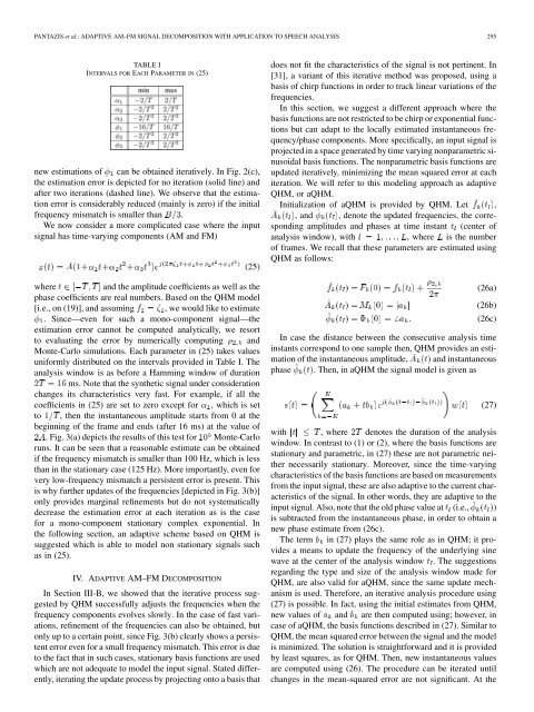
TABLE I<br />
INTERVALS FOR EACH PARAMETER IN (25)<br />
new estimations of can be obtained iteratively. In Fig. 2(c),<br />
the estimation error is depicted for no iteration (solid line) and<br />
after two iterations (dashed line). We observe that the estimation<br />
error is considerably reduced (mainly is zero) if the initial<br />
frequency mismatch is smaller than .<br />
We now consider a more complicated case where the input<br />
signal has time-varying components (AM and FM)<br />
(25)<br />
where<br />
and the amplitude coefficients as well as the<br />
phase coefficients are real numbers. Based on the QHM model<br />
[i.e., on (19)], and assuming , we would like <strong>to</strong> estimate<br />
. Since—even for such a mono-component signal—the<br />
estimation error cannot be computed analytically, we resort<br />
<strong>to</strong> evaluating the error by numerically computing and<br />
Monte-Carlo simulations. Each parameter in (25) takes values<br />
uniformly distributed on the intervals provided in Table I. The<br />
analysis window is as before a Hamming window of duration<br />
ms. Note that the synthetic signal under consideration<br />
changes its characteristics very fast. For example, if all the<br />
coefficients in (25) are set <strong>to</strong> zero except for , which is set<br />
<strong>to</strong> , then the instantaneous amplitude starts from 0 at the<br />
beginning of the frame and ends (after 16 ms) at the value of<br />
. Fig. 3(a) depicts the results of this test for Monte-Carlo<br />
runs. It can be seen that a reasonable estimate can be obtained<br />
if the frequency mismatch is smaller than 100 Hz, which is less<br />
than in the stationary case (125 Hz). More importantly, even for<br />
very low-frequency mismatch a persistent error is present. This<br />
is why further updates of the frequencies [depicted in Fig. 3(b)]<br />
only provides marginal refinements but do not systematically<br />
decrease the estimation error at each iteration as is the case<br />
for a mono-component stationary complex exponential. In<br />
the following section, an adaptive scheme based on QHM is<br />
suggested which is able <strong>to</strong> model non stationary signals such<br />
as in (25).<br />
IV. ADAPTIVE <strong>AM–FM</strong> DECOMPOSITION<br />
In Section III-B, we showed that the iterative process suggested<br />
by QHM successfully adjusts the frequencies when the<br />
frequency components evolves slowly. In the case of fast variations,<br />
refinement of the frequencies can also be obtained, but<br />
only up <strong>to</strong> a certain point, since Fig. 3(b) clearly shows a persistent<br />
error even for a small frequency mismatch. This error is due<br />
<strong>to</strong> the fact that in such cases, stationary basis functions are used<br />
which are not adequate <strong>to</strong> model the input signal. Stated differently,<br />
iterating the update process by projecting on<strong>to</strong> a basis that<br />
does not fit the characteristics of the signal is not pertinent. In<br />
[31], a variant of this iterative method was proposed, using a<br />
basis of chirp functions in order <strong>to</strong> track linear variations of the<br />
frequencies.<br />
In this section, we suggest a different approach where the<br />
basis functions are not restricted <strong>to</strong> be chirp or exponential functions<br />
but can adapt <strong>to</strong> the locally estimated instantaneous frequency/phase<br />
components. More specifically, an input signal is<br />
projected in a space generated by time varying nonparametric sinusoidal<br />
basis functions. The nonparametric basis functions are<br />
updated iteratively, minimizing the mean squared error at each<br />
iteration. We will refer <strong>to</strong> this modeling approach as adaptive<br />
QHM, or aQHM.<br />
Initialization of aQHM is provided by QHM. Let ,<br />
, and , denote the updated frequencies, the corresponding<br />
amplitudes and phases at time instant (center of<br />
analysis window), with , where is the number<br />
of frames. We recall that these parameters are estimated using<br />
QHM as follows:<br />
(26a)<br />
(26b)<br />
(26c)<br />
In case the distance between the consecutive analysis time<br />
instants correspond <strong>to</strong> one sample then, QHM provides an estimation<br />
of the instantaneous amplitude, and instantaneous<br />
phase . Then, in aQHM the signal model is given as<br />
(27)<br />
with , where denotes the duration of the analysis<br />
window. In contrast <strong>to</strong> (1) or (2), where the basis functions are<br />
stationary and parametric, in (27) these are not parametric neither<br />
necessarily stationary. Moreover, since the time-varying<br />
characteristics of the basis functions are based on measurements<br />
from the input signal, these are also adaptive <strong>to</strong> the current characteristics<br />
of the signal. In other words, they are adaptive <strong>to</strong> the<br />
input signal. Also, note that the old phase value at (i.e., )<br />
is subtracted from the instantaneous phase, in order <strong>to</strong> obtain a<br />
new phase estimate from (26c).<br />
The term in (27) plays the same role as in QHM; it provides<br />
a means <strong>to</strong> update the frequency of the underlying sine<br />
wave at the center of the analysis window . The suggestions<br />
regarding the type and size of the analysis window made for<br />
QHM, are also valid for aQHM, since the same update mechanism<br />
is used. Therefore, an iterative analysis procedure using<br />
(27) is possible. In fact, using the initial estimates from QHM,<br />
new values of and are then computed using; however, in<br />
case of aQHM, the basis functions described in (27). Similar <strong>to</strong><br />
QHM, the mean squared error between the signal and the model<br />
is minimized. The solution is straightforward and it is provided<br />
by least squares, as for QHM. Then, new instantaneous values<br />
are computed using (26). The procedure can be iterated until<br />
changes in the mean-squared error are not significant. At the