Adaptive AM–FM Signal Decomposition With Application to ... - ICS

More documents

Recommendations

Info

PANTAZIS et al.: ADAPTIVE AM–FM SIGNAL DECOMPOSITION WITH APPLICATION TO SPEECH ANALYSIS 291 to balance the time and frequency resolution requests of speech signals by choosing the length of the analysis window and the frame rate. However, when fast transitions occur in amplitude and/or in frequency, the sinusoidal model is inadequate for tracking the AM–FM components of the signal, since this model assumes speech stationarity within an analysis frame. In this paper, we suggest an adaptive method for estimating the instantaneous components of voiced speech signals. The suggested approach can also be applied to other time-varying multi-component AM–FM signals like music signals, signals (or calls) generated by marine mammals, birds, etc. The suggested method is based on a model initially introduced by Laroche et al. for audio modeling of percussive sounds [25] and for speech analysis [1]. In [26], the model was reintroduced revealing its main properties: it was shown that the model is equivalent to a time-varying quasi-harmonic representation of speech. In the following, this model will be referred to as Quasi-Harmonic Model (QHM). In this paper, we first show the robustness of QHM as frequency estimator. QHM assumes that an initial estimate for the frequencies of the components is provided as well as that the number of components is known a priori. Then, the remaining parameters are estimated by minimizing the mean squared error between the speech signal and the model which leads to a least squares (LS) solution. In practice, however, a frequency mismatch between the original and the initial estimates of frequencies is inevitable. Reformulating the QHM representation, we show that QHM provides a mechanism for iteratively estimating the frequency mismatch and consequently improving the amplitude estimation in the mean-squared sense. Robustness issues of the frequency mismatch estimation algorithm are discussed and bounds on the magnitude of frequency mismatch for which the algorithm converges are provided. Similar to sinusoidal modeling, QHM assumes speech to be locally stationary. In the case of signals exhibiting strong AM–FM, experiments show that QHM is limited in the sense that it can capture variations of frequencies and amplitudes but only up to a certain point. To overcome this limitation, we expand QHM to a novel speech representation referred to as adaptive QHM, or aQHM, where speech is not assumed to be locally stationary, taking into account the trajectories of the instantaneous frequencies. Then, the speech signal is projected in a space generated by time varying nonparametric sinusoidal basis functions. Therefore, the basis functions are adapted to the local characteristics of the input signal. The basis functions are updated by minimizing the mean squared error between the input signal and the aQHM model, at each adaptation step. This leads to a non-parametric AM–FM decomposition algorithm for speech signals. This is indeed, one key difference between aQHM and other AM–FM decomposition approaches like those suggested in [20], [22], where the amplitude and/or phase functions are represented by linear parametric models. In that sense, aQHM suggests a more flexible AM–FM decomposition algorithm. Another key difference between these approaches and aQHM, lies in the fact that aQHM takes into account the specific properties of voiced speech signals (i.e., quasi-harmonic structure). In that sense, aQHM suggests a representation that is more suitable for speech than the generic models suggested in [20] and [22]. On the other hand, the suggested representation can be applied in a straightforward way on other multicomponent signals, simply by adjusting accordingly the expected distribution of the frequency information. For instance, in the case of singing voice or music, or certain marine biologic sounds, frequencies are expected to have a quasi-harmonic structure. In other cases, however, signals may contain a sparse and uncorrelated frequency content. In any case, prior knowledge about the structure and properties of the input signal may reduce the complexity of models while increasing their modeling efficiency. The Sinusoidal Model (SM) suggests a maximum-likelihood frequency estimator, assuming a harmonic structure for the speech waveform. This leads to a simple peak-picking algorithm for estimating, at the analysis stage, the parameters of the model from the short-time Fourier transform of the signal [24]. Then at the synthesis stage, parametric models for the instantaneous amplitude (linear model) and phase (cubic model) are used for the signal reconstruction. Comparisons between SM, QHM, and aQHM were conducted for validation purposes, on synthetic signals under various noise conditions, while for evaluation we used voiced speech signals. Results show that the suggested approaches outperform SM in terms of accuracy in parameters estimation (for synthetic signals) and in signal-to-reconstruction error ratio (for speech signals). The organization of the paper is as follows. Section II presents an overview of QHM and reveals its main time and frequency properties showing that under certain conditions, QHM may be used to enhance frequency estimation. In Section III, these conditions are further examined and bounds where such an enhancement is possible in the context of QHM, are provided. The iterative adaptive AM–FM decomposition algorithm based on aQHM is presented in Section IV. The validity of the proposed approach, its robustness under noisy conditions, as well as its comparison with the SM on synthetic AM–FM signals are shown in Section V. To further support our suggestions, results of signal reconstruction on voiced speech signals from many speakers using SM, QHM, and aQHM are provided in Section VI. Section VII concludes the paper and discusses future directions of this work. II. QUASI-HARMONIC MODEL A. Overview QHM Within an analysis window, the deterministic (i.e., quasi-harmonic) component of a speech signal is modeled as ([27, Ch. 4]) where is the fundamental frequency of the harmonic signal, specifies the order of the model, i.e., the number of harmonics, are the complex amplitudes, are the complex slopes, and denotes the analysis window which is typically a Hamming window and zero outside a symmetric interval . Thus, will always denote the center of the analysis window. Note that for real signals such as speech, audio, (1)
292 IEEE TRANSACTIONS ON AUDIO, SPEECH, AND LANGUAGE PROCESSING, VOL. 19, NO. 2, FEBRUARY 2011 etc., and , where is the conjugate operator. This model is an extension to the classic harmonic model in which the term is omitted [27]. As a result, it follows that the signal in (1) is projected onto the complex exponential functions, as in the simple harmonic case, and to functions of type . It is worth noting that the model in (1) can also be written for nonharmonically related frequency components. Therefore, a more general model can be expressed as (2) where will be referred to as initial estimates of the frequencies that will be considered to be known. Initial frequencies (or ) are considered to be known but not necessary optimal in representing the input signal in the mean squared error sense. For speech as well as for music signals, this is quite often the case. Assuming that the speech signal is defined on , the estimation of the model parameters is performed into two steps. At first, the fundamental frequency, and the number of harmonic components, , are estimated using spectral and autocorrelation information as described in [27]. Then, the computation of is performed by minimizing a mean squared error which leads to a simple least squares solution [27]. The same procedure is applied if the initial estimates of frequencies are not restricted to be multiples of a fundamental frequency. In this case, frequencies may be obtained by peak picking the magnitude spectrum of the Fourier transform of the input signal as suggested in [24]. In the following, we will not restrict the analysis to , unless otherwise mentioned. From (2), it is easily seen that the instantaneous amplitude of each component is a time-varying function given by where and denote the real and the imaginary parts of , respectively. 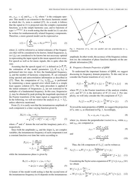Since both the amplitudes and the slopes are complex variables, the instantaneous frequency of each component is not a constant function over time but varies according to while the instantaneous phase is given by A feature of the model worth noting is that the second term of the instantaneous frequency in (4) depends on the instantaneous (3) (4) (5) Fig. 1. Projection of b component. into one parallel and one perpendicular to a amplitude. In other words, the accuracy of the frequency estimation (or, the estimation of phase function) depends on the amplitude information [28]. B. Frequency-Domain Properties of QHM To understand the important features of QHM, we suggest discussing its frequency domain properties. To this end, let us consider the Fourier transform of in (2) where is the Fourier transform of the analysis window, , and is the derivative of over . For simplicity, we will only consider the th component of To reveal the main properties of QHM, we suggest the projection of onto as illustrated in Fig. 1. Accordingly, where denotes the perpendicular (vector) to , while and are computed as and Thus, the th component of can be written as Considering the Taylor series expansion of we obtain (6) (7) (8) (9) (10) (11) (12)
Page 1: 290 IEEE TRANSACTIONS ON AUDIO, SPE
Page 5 and 6: 294 IEEE TRANSACTIONS ON AUDIO, SPE
Page 11: 300 IEEE TRANSACTIONS ON AUDIO, SPE

Adaptive AM–FM Signal Decomposition With Application to ... - ICS

Create successful ePaper yourself

Delete template?

Save as template?