The Finite Element Method for the Analysis of Non-Linear and ...

The Finite Element Method for the Analysis of
Non-Linear and Dynamic Systems
Prof. Dr. Eleni Chatzi
Lecture 1 - 20 September, 2010
Institute of Structural Engineering Method of Finite Elements II 1

Course Information
Instructor
Prof. Dr. Eleni Chatzi, email: chatzi@ibk.baug.ethz.ch
Office Hours: HIL E14.3, Wednesday 10:00-12:00 or by email
Assistant
Mohammad Miah, HIL E14.2, email: miah@ibk.baug.ethz.ch
Course Website
Lecture Notes and Homeworks will be posted at:
http://www.ibk.ethz.ch/ch/education
Suggested Reading
Finite Element Procedures by K.J. Bathe, Prentice Hall, 1996
Nonlinear Finite Elements for Continua and Structures by T.
Belytschko, W. K. Liu, and B. Moran, John Wiley and Sons, 2000
The Finite Element Method: Linear Static and Dynamic Finite
Element Analysis by T. J. R. Hughes, Dover Publications, 2000
Institute of Structural Engineering Method of Finite Elements II 2

Course Outline
Review of the Finite Element method - Introduction to
Non-Linear Analysis
Non-Linear Finite Elements in solids and Structural Mechanics
- Overview of Solution Methods
- Continuum Mechanics & Finite Deformations
- Lagrangian Formulation
- Structural Elements
Dynamical Finite Element Calculations
- Integration Methods
- Mode Superposition
Eigenvalue Problems
Special Topics
- Extended Finite Elements, Multigrid Methods, Meshless Methods
Institute of Structural Engineering Method of Finite Elements II 3

Grading Policy
Homeworks (60%) - Class Project (40%)
Homework
Project
Homeworks are due in class 2 weeks after assignment
Computer Assignments may be done using any coding language
(MATLAB, Fortran, C, MAPLE) - example code will be provided in
MATLAB
Simulation of the non-linear behavior of a concrete column under
cyclic loading
Students can work in groups of two and can assist with the
experimental setup
A final written report by each team will be submitted at the end of
the class
Institute of Structural Engineering Method of Finite Elements II 4

Review of the Finite Element Method (FEM)
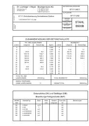
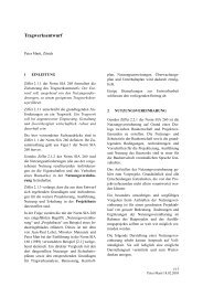
Classification of Engineering Systems
Discrete
Continuous
q|y+dy
h 1
q|x
dy
q|x+dx
dx
q|y
h 2
L
Flow
of water
Permeable Soil
F = KX
Direct Stiffness Method
k
( )
∂ 2 φ
∂ 2 x + ∂2 φ
∂ 2 y
Impermeable Rock
Laplace Equation
= 0
FEM: Numerical Technique for solution of continuous systems.
We will use a displacement based formulation and a stiffness based solution
(direct stiffness method).
Institute of Structural Engineering Method of Finite Elements II 5

Review of the Finite Element Method (FEM)
Differential Formulation (Strong Form)
Obtained through equilibrium and Constitutive Requirements
Governing Differential Equation ex: general 2nd order PDE
A(x, y) ∂2 u
∂ 2 x + 2B(x, y) ∂2 u
∂x∂y + C(x, u
y)∂2 ∂ 2 y
= φ(x, y, u,
∂u
∂y , ∂u
∂y )
Problem Classification
B 2 − AC < 0 ⇒ elliptic
B 2 − AC = 0 ⇒
parabolic
B 2 − AC > 0 ⇒
hyperbolic
Boundary Condition Classification
Essential (Dirichlet): u(x 0 , y 0 ) = u 0
order m − 1 at most for C m−1
Natural (Neumann): ∂u
∂y (x 0, y 0 ) = ˙u 0
order m to 2m − 1 for C m−1
Institute of Structural Engineering Method of Finite Elements II 6

Strong Form - 1D FEM
Consider the following 1D strong form
d
dx (c(x)du dx ) + f(x) = 0
− c(0) d dx u(0) = h
u(L) = 0
(Neumann BC)
(Dirichlet BC)
Physical Problem (1D) Diff. Equation Quantities
One dimensional Heat
flow
Axially Loaded Bar
d dT
Ak
dx dx + Q = 0
d du
AE
dx dx + b = 0
T=temperature
A=area
k=thermal
conductivity
Q=heat supply
u=displacement
A=area
E=Young’s
modulus
B=axial loading
Constitutive
Law
Fourier
q = −k dT/dx
q = heat flux
Hooke
σ = Edu/dx
σ = stress
Institute of Structural Engineering Method of Finite Elements II 7

Weak Form - 1D FEM
From Strong Form to Weak form - Approach #1
Principle of Virtual Work:
For any compatible small virtual displacements imposed on the body in its
state of equilibrium, the total internal virtual work is equal to the total
external virtual work.
∫
W int =
where
Ω
∫
¯ɛ T τ dΩ = W ext =
Ω
∫
ū T bdΩ + ū ST T S dΓ + ∑
Γ
i
ū iT R C
i
T S : surface traction (along boundary Γ)
b: body force per unit area
R C : nodal loads
ū: virtual displacement
¯ɛ: virtual strain
τ : stresses
Institute of Structural Engineering Method of Finite Elements II 8

Weak Form - 1D FEM
From Strong Form to Weak form - Approach #2
Principle of Minimum Potential Energy:
Applies to elastic problems where since the elasticity matrix is positive
definite, hence the energy functional Π has a minimum (stable equilibrium).
Approach #1 applies in general.
The potential energy Π is defined as the strain energy U minus the work of
the external loads W
Π = U − W
U = 1 ∫
ɛ T CɛdΩ
2 Ω
∫
∫
W = ū T bdΩ + ū ST T s dΓ T + ∑
Ω
Γ T i
ū T i R C
i
(b T s , R C as defined previously)
Institute of Structural Engineering Method of Finite Elements II 9

Weak Form - 1D FEM
3. Derive Weak form from Strong form
Given an arbitrary weight function w, where
S = {u|u ∈ C 0 , u(l) = 0}, S 0 = {w|w ∈ C 0 , w(l) = 0}
C 0 is the collection of all continuous functions.
Multiplying by w and integrating over Ω
∫ l
0
w(x)[(c(x)u ′ (x)) ′ + f (x)]dx = 0
[w(0)(c(0)u ′ (0) + h] = 0
Institute of Structural Engineering Method of Finite Elements II 10

Weak Form - 1D FEM
Using the divergence theorem (integration by parts) we reduce the
order of the differential:
∫ l
0
∫ l
wg ′ dx = [wg] l 0 − gw ′ dx
0
The weak form is then written
Find u(x) ∈ S such that :
∫ l
0
wcu ′ dx =
∫ l
0
wfdx + w(0)h
S = {u|u ∈ C 0 , u(l) = 0}
S 0 = {w|w ∈ C 0 , w(l) = 0}
Institute of Structural Engineering Method of Finite Elements II 11

FE formulation: Discretization
Divide the body into finite elements, e, connected to each other
through nodes
e
x 1
e
x 2
e
Replace the integral as sum over the elements:
[
∑ ∫ x e ∫ ]
2
x e
w ′ cu ′ 2
dx − wfdx − w(0)h = 0
x1
e x1
e
e
Institute of Structural Engineering Method of Finite Elements II 12

1D FE formulation: Galerkin’s Method
Galerkin’s method assumes that the approximate solution, u, can be
expressed as
u(x) ≈ u h (x) = ∑ i
N i (x)u i = N(x)u
The weighting function, w is chosen to be of the same form as u
w(x) ≈ w h (x) = ∑ i
N i (x)w i = N(w)w
N = [N 1 N 2 ] u = [u 1 u 2 ] T w = [w 1 w 2 ] T (for 2 nodes)
Shape function Properties:
Bounded and Continuous
One for each node
Ni e(x j e) = δ ij, where
{
1 if i = j
δ ij =
0 if i ≠ j
Institute of Structural Engineering Method of Finite Elements II 13

1D FE formulation: Galerkin’s Method
Substituting into the weak formulation and rearranging terms, we
finally obtain the following discrete system:
Ku = f
K = A e K e −→ K e =
∫ x e
2
x1
e
N Ț xcN ,x dx =
∫ x e
2
x1
e
B T cBdx
f = A e f e −→ f e =
∫ x e
2
x e 1
N T fdx + N T h| x=0
where A is not a sum but an assembly and , x denotes differentiation
with respect to x
Institute of Structural Engineering Method of Finite Elements II 14

1D FE formulation: Iso-Parametric Formulation
Iso-Parametric Mapping
x
x 1
e
x 2
e
−1 1
ξ
Shape Functions in Natural Coordinates
x(ξ) = ∑
N i (ξ)xi e = N 1 (ξ)x1 e + N 2 (ξ)x2
e
i=1,2
N 1 (ξ) = 1 2 (1 − ξ), N 2(ξ) = 1 (1 + ξ)
2
Institute of Structural Engineering Method of Finite Elements II 15

1D FE formulation: Iso-Parametric Formulation
Map the integrals to the natural domain −→ element stiffness matrix:
K e =
∫ x
e
2
x e 1
N Ț xcN ,xdx =
where N ,ξ = d dξ
∫ 1
−1
and x ,ξ = dx
dξ = x 2 e − x1
e
2
(N ,ξ ξ ,x) T c(N ,ξ ξ ,x)x ,ξ dξ
[ 1
]
(1 − ξ)
2
1
(1 + ξ) 2
=
[ −1
2
1
2
]
= h 2 = J (Jacobian)
ξ ,x = dξ
dx = J−1 = 2/h
From all the above,
[ ]
K e c 1 −1
=
x2 e − x 1
e −1 1
Similary, we obtain the element load vector:
f e =
∫ x
e
2
x e 1
N T fdx + N T h| x=0 =
∫ 1
−1
N T (ξ)fx ,ξ dξ + N T (x)h| x=0
Note: the iso-parametric mapping is only done for the integral.
Institute of Structural Engineering Method of Finite Elements II 16

Strong Form - 2D Linear Elasticity FEM
Governing Equations
Equilibrium Eq: ∇ s σ + b = 0 ∈ Ω
Kinematic Eq: ɛ = ∇ s u ∈ Ω
Constitutive Eq: σ = D · ɛ ∈ Ω
Traction B.C.: τ · n = T s ∈ Γ t
Displacement B.C: u = u Γ ∈ Γ u
Hooke’s Law - Constitutive Equation
Plane Stress
Plane Strain
τ zz = τ xz = τ yz = 0, ɛ zz ≠ 0 ɛ zz = γ xz = γ yz = 0, σ zz ≠ 0
⎡
⎤
⎡
D =
E 1 ν 0
1 − ν ν 0
⎣ ν 1 0 ⎦
E
D =
⎣ ν 1 − ν 0
1 − ν 2 (1 − ν)(1 + ν)
0 0
0 0
1−ν
2
1−2ν
2
⎤
⎦
Institute of Structural Engineering Method of Finite Elements II 17

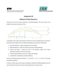
2D FE formulation: Discretization
Divide the body into finite elements connected to each other through
nodes
Institute of Structural Engineering Method of Finite Elements II 18

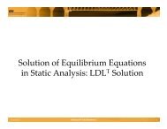
2D FE formulation: Iso-Parametric Formulation
Shape Functions in Natural Coordinates
N 1 (ξ, η) = 1 4 (1 − ξ)(1 − η), N 2(ξ, η) = 1 (1 + ξ)(1 − η)
4
N 3 (ξ, η) = 1 4 (1 + ξ)(1 + η), N 4(ξ, η) = 1 (1 − ξ)(1 + η)
4
Iso-parametric Mapping
x =
y =
4∑
N i (ξ, η)xi
e
i=1
4∑
i=1
N i (ξ, η)y e
i
Institute of Structural Engineering Method of Finite Elements II 19

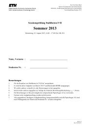
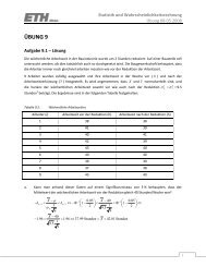
Bilinear Shape Functions
Institute of Structural Engineering Method of Finite Elements II 20

Appendix - Axially Loaded Bar Example
Constant End Load
Given: Length L, Section Area A, Young’s modulus E
Find: stresses and deformations.
Assumptions:
The cross-section of the bar does not change after loading.
The material is linear elastic, isotropic, and homogeneous.
The load is centric.
End-effects are not of interest to us.
Institute of Structural Engineering Method of Finite Elements II 22

Appendix - Axially Loaded Bar Example
Strength of Materials Approach
From equilibrium equation, axial force at random point x along the
bar is:
f(x) = R(= const) ⇒ σ(x) = R A
From constitutive equation (Hooke’s Law):
ɛ(x) = σ(x)
E
Hence, the deformation is obtained as:
= R
AE
δ(x) = ɛ(x)
x
⇒ δ(x) = Rx
AE
Institute of Structural Engineering Method of Finite Elements II 23

Appendix - Axially Loaded Bar Example
Linearly Distributed Axial Load
From equilibrium equation, axial force at random point x along the
bar is:
f(x) = R + a(L2 − x 2 )
( depends on x)
2
In order to now find stresses, deformations we have to repeat the
process for every point in the bar (computationally inefficient).
Institute of Structural Engineering Method of Finite Elements II 24

Appendix - Axially Loaded Bar Example
From equilibrium equation, for the infinitesimal element:
∆σ
dσ
Aσ = q(x)∆x + A(σ + ∆σ) ⇒ A }{{}
lim + q(x) = 0 ⇒ A
∆x dx + q(x) = 0
∆x→0
Also, ɛ = du
dx , ɛ = Eɛ, q(x) = ax ⇒ AE d 2 u
dx 2 + ax = 0
Strong Form
AE d 2 u
dx + ax = 0
2
u(0) = 0 essential BC
f(L) = R ⇒ AE du
dx ∣ = R natural BC
x=L
Analytical Solution
u(x) = u hom + u p ⇒ u(x) = C 1x + C 2 − ax 3
6AE
C 1, C 2 are determined from the BC
Institute of Structural Engineering Method of Finite Elements II 25

Appendix - Axially Loaded Bar Example
An analytical solution cannot always be found
Approximate Solution - The Galerkin Approach: Multiply by the weight function w and
integrate over the domain
Apply integration by parts
∫ L
0
∫ L
0
[
AE d2 u
dx 2 wdx = AE du ] l
dx w −
0
AE d2 u
dx 2 wdx = [
∫ L
∫
AE d2 u
L
0 dx 2 wdx + axwdx = 0
0
AE du
dx
∫ L
0
AE du dw
dx dx dx ⇒
(L)w(L) − AE
du
dx (0)w(0) ]
−
∫ L
0
AE du dw
dx dx dx
But from BC we have u(0) = 0, AE du (L)w(L) = Rw(L), therefore the approximate
dx
weak form can be written as
∫ L
AE du
∫
dw
L
0 dx dx dx = Rw(L) + axwdx
0
Institute of Structural Engineering Method of Finite Elements II 26

Appendix - Axially Loaded Bar Example
In Galerkin’s method we assume that the approximate solution, u can be expressed as
u(x) =
n∑
u j N j (x)
w is chosen to be of the same form as the approximate solution (but with arbitrary
coefficients w i ),
w(x) =
j=1
n∑
w i N i (x)
i=1
Plug u(x),w(x) into the approximate weak form:
∫ L n∑ dN j (x)
AE u j
0
dx
j=1
n∑
i=1
w i
dN i (x)
dx
w i is arbitrary, so the above has to hold ∀ w i :
n∑
∫ L n∑
dx = R w i N i (L) + ax w i N i (x)dx
i=1
0
i=1
n∑
[∫ L dN j (x)
AE dN ]
∫
i (x)
L
dx u j = RN i (L) + axN i (x)dx
j=1
0 dx dx
0
i = 1 . . . n
which is a system of n equations that can be solved for the unknown coefficients u j .
Institute of Structural Engineering Method of Finite Elements II 27

Appendix - Axially Loaded Bar Example
The matrix form of the previous system can be expressed as
K ij u j = f i where K ij =
and f i = RN i (L) +
∫ L
0
∫ L
0
dN j (x)
dx
axN i (x)dx
AE dN i(x)
dx
dx
Finite Element Solution - using 2 discrete elements, of length h (3 nodes)
From the[ iso-parametric ] formulation we know the element stiffness matrix
1 −1
K e = AE . Assembling the element stiffness matrices we get:
h −1 1
⎡
K tot = ⎣
K11 e K12 1 0
K12 1 K22 1 + K11 2 K12
2
0 K12 2 K22
2
⎤
⎦ ⇒
K tot = AE h
⎡
⎣
1 −1 0
−1 2 −1
0 −1 1
⎤
⎦
Institute of Structural Engineering Method of Finite Elements II 28