Randomized Algorithms

CS 124 Section #7 Randomized Algorithms 4/7/13
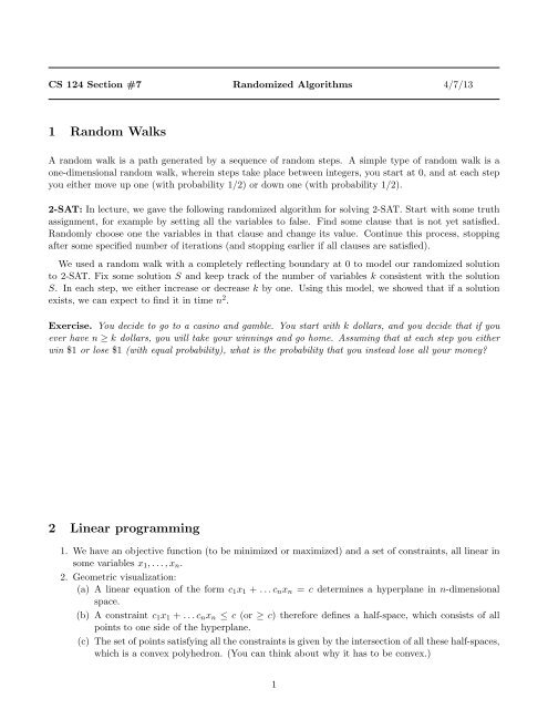
1 Random Walks
A random walk is a path generated by a sequence of random steps. A simple type of random walk is a
one-dimensional random walk, wherein steps take place between integers, you start at 0, and at each step
you either move up one (with probability 1/2) or down one (with probability 1/2).
2-SAT: In lecture, we gave the following randomized algorithm for solving 2-SAT. Start with some truth
assignment, for example by setting all the variables to false. Find some clause that is not yet satisfied.
Randomly choose one the variables in that clause and change its value. Continue this process, stopping
after some specified number of iterations (and stopping earlier if all clauses are satisfied).
We used a random walk with a completely reflecting boundary at 0 to model our randomized solution
to 2-SAT. Fix some solution S and keep track of the number of variables k consistent with the solution
S. In each step, we either increase or decrease k by one. Using this model, we showed that if a solution
exists, we can expect to find it in time n 2 .
Exercise. You decide to go to a casino and gamble. You start with k dollars, and you decide that if you
ever have n ≥ k dollars, you will take your winnings and go home. Assuming that at each step you either
win $1 or lose $1 (with equal probability), what is the probability that you instead lose all your money?
2 Linear programming
1. We have an objective function (to be minimized or maximized) and a set of constraints, all linear in
some variables x 1 , . . . , x n .
2. Geometric visualization:
(a) A linear equation of the form c 1 x 1 + . . . c n x n = c determines a hyperplane in n-dimensional
space.
(b) A constraint c 1 x 1 + . . . c n x n ≤ c (or ≥ c) therefore defines a half-space, which consists of all
points to one side of the hyperplane.
(c) The set of points satisfying all the constraints is given by the intersection of all these half-spaces,
which is a convex polyhedron. (You can think about why it has to be convex.)
1

(d) The objective function, a 1 x 1 +. . .+a n x n , can be thought of as a moveable hyperplane: We want
to find the highest (maximization) or lowest (minimization) value of α such that the hyperplane
a 1 x 1 + . . . + a n x n = α still intersects the polyhedron. Therefore the optimum occurs at a corner
of the polyhedron, which is why the simplex algorithm works.
Exercise. Express the following problem as a linear programming problem: A farmer has 10 acres to plant
in wheat and rye. He has to plant at least 7 acres. He has $1200 to spend; each acre of wheat costs $200
to plant and each acre of rye costs $100 to plant. Moreover, the farmer has to get the planting done in 12
hours, and it takes an hour to plant an acre of wheat and 2 hours to plant an acre of rye. If the profit is
$500 per acre of wheat and $300 per acre of rye, how many acres of each should be planted to maximize
profits?
Exercise. Express the following problem as a linear programming problem: A gold processor has two
sources of gold ore, source A and source B. In order to keep his plant running, at least three tons of ore
must be processed each day. Ore from source A costs $20 per ton to process, and ore from source B costs
$10 per ton to process. Costs must be kept to less than $80 per day. Moreover, Federal Regulations require
that the amount of ore from source B cannot exceed twice the amount of ore from source A. If ore from
source A yields 2 oz. of gold per ton, and ore from source B yields 3 oz. of gold per ton, how many tons of
ore from both sources must be processed each day to maximize the amount of gold extracted subject to the
above constraints?
2

3 Network flows
3.1 Simplex algorithm for network flows
1. Simple example:
S
1
T
2
3
A
Reduction to a linear program: Objective is to maximize f ST + f SA .
(a) Edge constraints: f ST ≤ 1, f SA ≤ 2, f AT ≤ 3, all are ≥ 0.
(b) Conservation of flow: f SA = f AT .
3.2 Max flow / min cut
1. Network: represented by a directed graph whose edge weights are flow capacities and whose vertices
include a start vertex S and an end-vertex T
2. Maximum flow of a network: the maximal flow that can pass from S to T .
3. Minimum cut of a network: a set of nodes containing S but not T , such that the sum of the capacities
of the edges exiting the set is minimized.
4. Maximum flow is equal to minimum cut: Maximum flow ≤ minimum cut is clear. Maximum
flow ≥ minimum cut comes from the augmenting paths algorithm: When there are no more augmenting
paths to be found, all the vertices reachable from S in the residual network form a cut. All
edges crossing this cut must have zero residual capacity, which means the flow is at least the sum of
their original capacities, which in turn is at least the flow of the minimum cut.
5. Residual flow: To form the residual network, we consider all edges e = (u, v) in the graph as well
as the reverse edges ē = (v, u).
(a) Any edge that is not part of the original graph is given capacity 0.
(b) If f(e) denotes the flow going across e, we set f(ē) = −f(e).
(c) The residual capacity of an edge is c(e) − f(e).
In particular, if e is an edge in the original graph with capacity c(e) = c (and with ē not in the
graph), and we ship flow f ≤ c across e, then e has residual capacity c − f. The reverse edge ē then
has residual capacity 0 − (−f) = f.
Exercise. Perform the augmenting paths algorithm on this example, showing the residual graph at each
step. What is the min-cut of this network?
3

A
3
B
1
C
3
3
1 2
S
4
D
5 3
E
T
The augmentation-based max-flow algorithm is called the Ford-Fulkerson method. Ford-Fulkerson doesn’t
specify how augmenting paths are to be found. The BFS-based approach referred to in lecture is known
as Edmonds-Karp and runs in time O(V E 2 ), even for non-integer capacities. In general, the method of
finding augmenting paths affects runtime. In a network with irrational capacities, it is possible to choose
augmenting paths such that Ford-Fulkerson never terminates.
Exercise. Challenge: Give an example of a network for which Ford-Fulkerson does not terminate.
4 LP duality, games
Linear programming problems have the duality property: that is, any LP maximization problem can be
written as a LP minimization problem whose optimum value is the same as that of the maximization
problem’s. (The same is clearly true vice-versa).
We have seen duality in the max-flow/min-cut problem and in matrix games (where the duality result is
called the min-max theorem). To translate from a LP problem to its dual:
1. Transpose the coefficient matrix.
2. Invert maximization to minimization.
3. Switch the RHS and the objective function.
4. Introduce a nonnegative variable for each inequality and an unrestricted one for each equality.
5. For each nonnegative variable introduce a ≥ constraint, and for each unrestricted variable introduce
a = constraint.
4

Exercise. Consider the following zero-sum game, where the entries denote the payoffs of the row player:
( 3 −1
) 2
1 2 −2
Write the column player’s maximization problem as a LP problem. Practice writing the dual LP “mechanically,”
and check the correctness of your answer by writing the row player’s minimization problem as a
LP problem.
Exercise. Now find the equilibrium of this game.
5