pdf-File - IAG - Universität Stuttgart

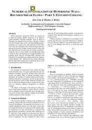
46th AIAA Aerospace Sciences Meeting and Exhibit
7 - 10 January 2008, Reno, Nevada
AIAA 2008-763
Direct Numerical Simulation of a Square-Notched
Trailing Edge for Jet-Noise Reduction
Andreas Babucke ∗ , Markus J. Kloker † and Ulrich Rist ‡
Institut für Aerodynamik und Gasdynamik, Universität Stuttgart, D-70550, Germany
Sound generation of a subsonic laminar jet has been investigated using direct numerical
simulation (DNS). The simulation includes the nozzle end, modelled by a finite flat splitter
plate with Mach numbers of Ma I = 0.8 above and Ma I = 0.2 below the plate. Behind the
nozzle end, a combination of wake and mixing layer develops. Due to its instability, roll up
and pairing of spanwise vortices occur, with the vortex pairing being the major acoustic
source. As a first approach for noise reduction, a rectangular notch at the trailing edge
is investigated. It generates longitudinal vortices and a spanwise deformation of the flow
downstream of the nozzle end. This leads to a an early breakdown of the large spanwise
vortices and accumulations of small-scale structures. The emitted sound is compared with
a two-dimensional simulation performed earlier. 2
k ∗
Nomenclature
dimensionless wavenumber: k ∗ = k · ∆x
Ma Mach number
p pressure
Re Reynolds number
t time
u, v, w velocity components in x, y and z direction, respectively
x, y, z streamwise, normal and spanwise direction, respectively
α streamwise wavenumber (α r ) and spatial amplification rate α i
γ spanwise wavenumber γ = 2π/λ z
δ 1 displacement thickness
µ viscosity
ρ density
ω angular frequency: ω = 2π · f
Subscript
I, II upper and lower stream, respectively
r, i real and imaginary part, respectively
I. Introduction
Noise reduction is of special interest for many technical problems, as high acoustic loads lead to a reduced
quality of life and may cause stress for persons concerned permanently. The current investigation focuses
on jet noise as it is a major noise source of aircrafts. As the major airports are typically located in highly
populated areas, noise reduction would improve the situation of many people. Direct aeroacoustic simulations
are a relatively new field in computational fluid dynamics, facing several difficulties due to largely different
scales. The hydrodynamic fluctuations are small-scale structures containing high energy compared to the
acoustics with relatively long wavelengths and small amplitudes. Therefore, high resolution is required to
∗ Research Assistant
† Senior Research Scientist
‡ Professor
1 of 11
American Institute of Aeronautics and Astronautics
Copyright © 2008 by Andreas Babucke. Published by the American Institute of Aeronautics and Astronautics, Inc., with permission.

compute the noise sources accurately. On the other hand a large computational domain is necessary to
obtain the relevant portions of the acoustic far-field. Due to the small amplitudes of the emitted noise,
boundary conditions have to be chosen carefully, in order not to spoil the acoustic field with reflections.
Up to now, large-eddy or direct numerical simulations of jet noise have been focusing on either pure
mixing layers 1,4,7 or low Reynolds number jets, 8 where an S-shaped velocity profile is prescribed at the
inflow. Our approach is to include the nozzle end, modelled by a thin finite flat plate with two different
free-stream velocities above and below. Including the nozzle end shifts the problem to a more realistic
configuration, leading to a combination of wake and mixing layer behind the splitter plate. Additionally,
wall-bounded actuators for noise reduction can be tested without the constraint to model them by artifical
volume forces. In the current investigation, a passive ’actuator’ is considered as a first realistic approach for
noise reduction.
II.A.
DNS code
II. Numerical Method
The simulation is carried out using the DNS code NS3D. 3 It solves the three-dimensional unsteady compressible
Navier-Stokes equations on multiple domains. The purpose of domain decomposition is not only
to increase computational performance, the combination with grid transformation and modular boundary
conditions allows to compute a wider range of problems. Computation is done in non-dimensional quantities:
velocities are normalized by the reference velocity U ∞ and all other quantities by their freestream values,
marked with the subscript ∞. Length scales are made dimensionless with a reference length L and the
time t with L/U ∞ , where the overbar denotes dimensional values. Temperature dependence of viscosity µ
is modelled using the Sutherland law:
µ(T) = µ(T ∞ ) · T 3/2 · 1 + T s
T + T s
, (1)
where T s = 110.4K/T ∞ and µ(T ∞ = 280K) = 1.735 · 10 −5 kg/(ms). Thermal conductivity ϑ is obtained by
assuming a constant Prandtl number Pr = c p µ/ϑ = 0.71 and a constant heat capacity c p . The most characteristic
parameters describing a compressible viscous flow-field are the Reynolds number Re = ρ ∞ U ∞ L/µ ∞
and the Mach number Ma = U ∞ /c ∞ with c being the speed of sound.
We use the conservative formulation of the Navier-Stokes equations which results in the solution vector
Q = [ρ, ρu, ρv, ρw, E] containing the density, the three momentum densities, and the total energy per volume
E = ρ · c v · T + ρ 2 · (u 2 + v 2 + w 2) . The simulation is carried out in a rectangular domain with x, y, z being
the coordinates in streamwise, normal and spanwise direction, respectively. A typical setup for jet-noise
computations is shown in figure 1.
y
z
x
0000000000000000
1111111111111111
0000000000000000
1111111111111111
0000000000000000
1111111111111111
0000000000000000
1111111111111111
0000000000000000
1111111111111111
0000000000000000
1111111111111111
0000000000000000
1111111111111111
0000000000000000
1111111111111111
0000000000000000
1111111111111111
0000000000000000
1111111111111111
0000000000000000
1111111111111111
0000000000000000
1111111111111111
0000000000000000
1111111111111111
0000000000000000
1111111111111111
0000000000000000
1111111111111111
0000000000000000
1111111111111111
0000000000000000
1111111111111111
0000000000000000
1111111111111111
0000000000000000
1111111111111111
0000000000000000
1111111111111111
0000000000000000
1111111111111111
λ z,0
Figure 1. Integration domain for jet noise computation with splitter plate and sponge zone.
Since the flow is assumed to be periodic in spanwise direction a spectral Fourier discretization in z
direction is used. The fundamental spanwise wavenumber γ 0 is given by the fundamental wavelength λ z,0
2 of 11
American Institute of Aeronautics and Astronautics

epresenting the spanwise width of the integration domain by γ 0 = 2π/λ z,0 . Spanwise derivatives are
computed by transforming the respective variable into Fourier space, multiplying its spectral components
with their wavenumbers (i · k · γ 0 ) for the first derivatives or square of their wavenumbers for the second
derivatives and transforming them back into physical space. Due to the non-linear terms in the Navier-Stokes
equations, higher harmonic spectral modes are generated at each timestep. To suppress aliasing, only 2/3 of
the maximum number of modes for a specific z resolution are used. 5 If a two-dimensional baseflow is used
and disturbances of u, v, ρ, T, p are symmetric and disturbances of w are antisymmetric, flow variables
are symmetric/antisymmetric with respect to z = 0. Therefore only half the number of points in spanwise
direction are needed (0 ≤ z ≤ λ z /2).
The spatial discretization in streamwise (x) and normal (y) direction is done by 6 th -order compact finite
differences. The tridiagonal equation systems of the compact finite differences are solved along multiple
domains using the pipelined Thomas algorithm. 3 To reduce the aliasing error, alternating up- and downwindbiased
finite differences are used for convective terms as proposed by Kloker. 10 The second derivatives are
evaluated directly which distinctly better resolves viscous terms compared to applying the first derivative
twice. 1 The time integration of the solution vector Q is done using the classical 4 th -order Runge-Kutta
scheme. 10 At each timestep and each intermediate level, the biasing of the finite differences for the convective
terms is changed. Mapping the physical x-y grid on an equidistant computational ξ-η grid allows arbitrary
grid transformations in the x-y plane.
II.B. Boundary conditions
For the jet-noise investigation, we use a one-dimensional characteristic boundary condition 9 at the freestream.
This allows outward-propagating acoustic waves to leave the domain. An additional damping zone forces
the flow variables smoothly to a steady state solution, avoiding reflections due to oblique waves. Having a
subsonic flow, we also use a characteristic boundary condition at the inflow, allowing upstream propagating
acoustic waves to leave the domain. Additionally amplitude and phase distributions from linear stability
theory can be prescribed to introduce defined disturbances. The outflow is the most crucial part as one
has to avoid high-amplitude structures passing the boundary and contaminating the sensitive acoustic field.
Therefore, a combination of grid stretching and spatial low-pass filtering along the x-direction is applied in
the sponge region. Disturbances become increasingly badly resolved as they propagate through the sponge
region. As the spatial filter depends on the step size in x-direction, perturbations are smoothly dissipated
before they reach the outflow boundary. This procedure shows very low reflections and has been already
applied by Colonius et al. 6
For the splitter plate representing the nozzle end, an isothermal boundary condition is used with the wall
temperature fixed at the value of the initial condition. The pressure is obtained by extrapolation from the
interior gridpoints. An extension of the wall boundary condition is the modified trailing edge, where the end
of the splitter plate is no more constant along the spanwise direction. As we have grid transformation only in
the x-y plane and not in z-direction, the spanwise dependency of the trailing edge is achieved by modifying
the connectivity of the affected domains. Instead of regularly prescribing the wall boundary condition along
the whole border of the respective subdomain, we can also define a region without wall. At these gridpoints,
the spatial derivatives in normal direction are recomputed, now using also values from the domain at the
other side of the splitter plate. The spanwise derivatives are computed in the same manner as inside the
flowfield with the Fourier-transformation being applied along the whole spanwise extent of the domain. The
modular boundary conditions, chosen because of flexibility, require explicit boundary conditions and by that
a non-compact finite-difference scheme, locally. Therefore explicit finite differences have been developed with
properties quite similar to the compact scheme used in the rest of the domain. According to Lele, 11 the
examination of the finite differences is based on the modified wavenumber kmod ∗ and its square k∗2
mod
for the
first and the second derivative, respectively. The numerical properties of the chosen 8 th -order scheme are
compared with standard explicit 6 th -order finite differences and the compact scheme of 6 th order, regularly
used in the flowfield. For the first derivative, the real and imaginary parts of the modified wavenumber kmod
∗
are shown in figure 2: the increase from order six to eight does not fully reach the good dispersion relation
of the 6 th -order compact scheme but at least increases the maximum of kmod ∗ by 10% compared with an
ad hoc explicit 6 th -order implementation. The imaginary part of the modified wavenumber, responsible for
dissipation, shows similar characteristics as the compact scheme with the same maximum as for the rest of
the domain. For the second derivative, shown by the square of the modified wavenumber kmod ∗2 in figure 3,
the increase of its order improves the properties of the explicit finite difference towards the compact scheme.
3 of 11
American Institute of Aeronautics and Astronautics

3
exact
Re(k* mod
) FD-O8
Re(k* mod
) CFD-O6
Re(k* mod
) FD-O6
Im(k* mod
) FD-O8
Im(k* mod
) CFD-O6
8
exact
Re(k* 2 mod
) FD O8
Re(k* 2 mod
) CFD O6
Re(k* 2 ) FD O6
mod
k* mod
2
k* 2 mod
6
4
1
2
0
0 0.5 1 1.5 2 2.5 3
k*
Figure 2. Real and imaginary part of the
modified wavenumber k ∗ mod for the first
derivative based on a wave with wave number
k ∗ = k · ∆x. Comparison of 8 th -order
explicit finite difference with 6 th -order explicit
and compact scheme.
0
0 0.5 1 1.5 2 2.5 3
k*
Figure 3. Square of the modified wavenumber
of the second derivative for a wave with
wave number k ∗ = k · ∆x. Comparison of
8 th -order explicit finite difference with 6 th -
order explicit and compact scheme.
II.C.
Initial condition
For the current investigation, an isothermal laminar subsonic jet with the Mach numbers Ma I = 0.8 for the
upper and Ma II = 0.2 for the lower stream has been selected. As both temperatures are equal (T 1 = T 2 =
280K), the ratio of the streamwise velocities is U I /U II = 4. This large factor leads to strong instabilities
behind the nozzle end. The Reynolds number Re = ρ ∞ U 1 δ 1,I /µ ∞ = 1000 is based on the displacement
thickness δ 1,I of the upper stream at the inflow. With δ 1,I (x 0 ) = 1, length scales are normalized with the
displacement thickness of the fast stream at the inflow. The boundary layer of the lower stream corresponds
to the same origin of the flat plate.
The cartesian grid is decomposed into sixteen subdomains: eight in streamwise and two in normal
direction. Each subdomain contains 325 x 425 x 65 points in x-, y- and z-direction, resulting in 42 spanwise
modes (dealiased) and a total number of 143.6 million gridpoints. The mesh is uniform in streamwise
direction with a step size of ∆x = 0.15 up to the sponge region, where the grid is highly stretched. In normal
direction, the finest step size is ∆y = 0.15 in the middle of the domain with a continuous stretching up to a
spacing of ∆y = 1.06 at the upper and lower boundaries. In spanwise direction, the grid is uniform with a
spacing of ∆z = 0.2454 which is equivalent to a spanwise wavenumber γ 0 = 0.2, where λ z /2 = π/γ 0 = 15.708
is the spanwise extent of the domain. The origin of the coordinate system (x = 0, y = 0) is located at the
end of the nozzle. Figure 4 shows the x-y plane of the integration domain, illustrating the grid stretching
and the domain decomposition. The nozzle end itself is modeled by a finite thin flat plate with a thickness
of one ∆y. Due to the vanishing thickness of the nozzle end, an isothermal boundary condition at the wall
has been chosen. The temperature of the plate is T wall = 296K, being the mean value of the adiabatic wall
temperatures of the two streams.
The initial condition along the flat plate is obtained from similarity solutions of the boundary-layer
equations. Further downstream, the compressible boundary-layer equations are integrated downstream,
providing a flow-field sufficient to serve as an initial condition and for linear stability theory. Due to the
geometrical discontinuity at the trailing edge, an ad-hoc solution of the boundary-layer equations shows a
peak in the wall-normal velocity v. Therefore, its value is smoothed around x = 0, providing a more realistic
flow field. Thus the characteristic boundary condition at the freestream can be linearized with respect to
the initial condition. The resulting streamwise velocity profiles of the initial condition are shown in figures 5
and 6. Behind the nozzle end, the flow field keeps its wake-like shape for a long range. As high amplification
rates occur here, the flow is already unsteady before a pure mixing layer has developed. This means that
the pure mixing layer investigated earlier 1,4,7 has to be considered as a rather theoretical approach.
4 of 11
American Institute of Aeronautics and Astronautics

0.4
0.2
y
0
100
-0.2
-0.4
-0.6
x
-0.5 0 0.5
y
0
-100
0 100 200 300
x
Figure 4. Integration domain in the x-y plane showing every 25 th grid line. The colour indicates the domain decomposition.
III. Linear Stability Theory
Spatial linear stability theory (LST) 12 is based on the linearization of the Navier-Stokes equations, split
into a steady two-dimensional baseflow and wavelike disturbances
Φ = ˆΦ (y) · e i(αx+γz−ωt) + c.c. (2)
with Φ = (u ′ , v ′ , w ′ , ρ ′ , T ′ , p ′ ) representing the set of fluctuations of the primitive variables. As only first
derivatives in time occur, the temporal problem, where the streamwise wavenumber α = α r is prescribed,
is solved first by a 4 th -order matrix solver providing the complex eigenvalues (ω r , ω i ), with ω r being the
frequency and ω i the temporal amplification. Once an amplified eigenvalue is found, the Wielandt iteration
iterates the temporal to the spatial problem by varying the spatial amplification −(α i ) such that ω i = 0. This
can also be done for a range of streamwise wavenumbers α r and x positions to obtain a stability diagram. A
selected spatial eigenvalue (α r , α i ) can be fed into the matrix solver to obatin the eigenfunction, being the
amplitude and phase distribution of the primitive variables along y. The eigenfunctions can be used directly
in the DNS-code for disturbance generation at the inflow.
As the flow is highly unsteady behind the nozzle end and enforcing an artificial steady state does not
work properly, we use the initial condition derived from the boundary-layer equations to compute eigenvalues
and eigenfunctions. According to figure 7, a fundamental angular frequency of ω 0 = 0.0688 was chosen for
the upper boundary layer. The amplification keeps almost constant in downstream direction. As the two
boundary layers emerge from the same position, the lower boundary layer is stable up to the nozzle end.
Behind the edge of the splitter plate, amplification rates 50 times higher than in the upper boundary layer
5 of 11
American Institute of Aeronautics and Astronautics

occur due to the inflection points of the streamwise-velocity profile. Maximum amplification in the mixing
layer takes place for a frequency of roughly three to four times of the fundamental frequency of the boundary
layer as illustrated in figure 8.
15
15
y
10
5
0
x = -97.5
Reδ 1
= 1000
y
10
5
0
x = 0 ... 96.75
-5
-5
-10
-10
-15
0 0.2 0.4 0.6 0.8 1
u
Figure 5. Profile of the streamwise velocity u
for the upper and lower boundary layer at the
inflow.
-15
0 0.2 0.4 0.6 0.8 1
u
Figure 6. Downstream evolution of the streamwise
velocity profile behind the nozzle end.
-0.01
0
-0.2
-0.1
ω 0
= 0.0688
x = 1.35
x = 13.35
α i
0.01
ω 0
= 0.0688
x = -0.15
x = -97.5
α i
0
0.1
0.05
ω
0.1 0.15
r
0.2
0.1
ω
0.2 0.3
r
Figure 7. Amplification rates of the upper
(fast) boundary layer given by linear stability
theory for various x−positions.
Figure 8. Amplification rates for various
x−positions behind the splitter plate predicted
by linear stability theory.
IV. DNS Results
For the pure mixing layer without splitter plate, 1 we already found that introducing a steady longitudinal
vortex leads to a break-up of the large spanwise vortices and may reduce the emitted sound originating from
vortex pairing. A variety of wall-mounted actuators are conceivable for the generation of streamwise vortices:
Our approach is to engrail the trailing edge of the splitter plate. Here, a rectangular spanwise profile of one
notch per spanwise wavelength with a depth of 10 in x-direction has been chosen. At the inflow of the upper
boundary layer, the flow is disturbed with the Tollmien-Schlichting (TS) wave (1, 0) with the fundamental
frequency ω 0 and an amplitude of û max = 0.005, being the same as for the two-dimensional simulation,
performed earlier. 2 The TS wave generates higher harmonics in the upper boundary layer, driving the rollup
of spanwise vortices (Kelvin-Helmholtz instability) and the subsequent vortex pairing behind the splitter
plate. An additional oblique wave (1, 1) with a small amplitude of û max = 0.0005 is intended to provide a
more realistic inflow disturbance than a purely two-dimensional forcing. A total number of 80000 timesteps
with ∆t = 0.018265 has been computed, corresponding to an non-dimensional elapsed time of t = 1461, with
the last four periods of the fundamental frequency used for analysis.
6 of 11
American Institute of Aeronautics and Astronautics

IV.A.
Flow Field
The instantaneous flowfield is illustrated in figure 9, showing the λ 2 vortex criterion. Small vortices emerge
from the longitudinal edges, slightly deforming the first spanwise vortex of the Kelvin-Helmholtz instability.
Further downstream, multiple streamwise vortices exist per λ z,0 , being twisted around the spanwise vortices.
This vortex interaction leads to a breakdown of the large spanwise vortices. From x ≈ 120 onwards, the
Kelvin-Helmholtz vortices known from two-dimensional investigations are now an accumulation of smallscale
structures. The spanwise vorticity at z = 0 for the serrated nozzle end and for the corresponding
two-dimensional simulation 2 is shown in figure 10. The initial roll up of the mixing layer is quite similar.
These generated Kelvin-Helmholtz vortices merge further downstream for the two-dimensional case. With
the rectangularly serrated trailing edge, the disintegration of the spanwise vortices begins at x ≈ 90 resulting
in a breakdown into smaller structures further downstream (x > 120).
Figure 9. Perspective view of the engrailed trailing edge and the vortical structures in the instantaneous flow field,
visualized by the isosurface λ 2 = −0.005. The distance from the plane of the splitter plate (y = 0) is colored from blue
(y < 0) to red (y > 0).
A spectral decomposition is shown in figures 11 and 12, based on the maximum of v along y. The normal
velocity has been chosen as it is less associated with upstream propagating sound. The modes are denoted
as (h, k) with h and k being the multiple of the fundamental frequency ω 0 and the spanwise wavenumber γ 0 ,
respectively. As figure 11 shows, the nonlinear interaction of the introduced disturbances (1, 0) and (1, 1) in
the upper boundary layer generates nonlinearly the mode (0, 1) up to an amplitude of ˆv = 2 · 10 −5 . From
x = −25 onwards, the upstream effect of the notch at the end of the splitter plate prevails. The engrailment
at the end of the splitter plate (−10 ≤ x ≤ 0) generates steady three-dimensional disturbances (0, k) with
peaks up to ˆv = 8 · 10 −3 at the corners. In the notch (7.8 ≤ z ≤ 23.6), the combination of wake and mixing
layer originates further upstream at x = −10 instead of x = 0. This results in a spanwise deformation,
corresponding to the disturbance (0, 1). Its amplitude decreases behind the splitter plate up to x = 15.
Higher harmonics in spanwise direction (0, 2) and (0, 4) are generated at the notch as well, but only mode
(0, 2) shows a similar upstream effect as mode (0, 1). Behind the splitter plate, the amplitudes of the first two
higher harmonics in spanwise direction stay almost constant at an amplitude of ˆv ≈ 6 ·10 −4 and ˆv ≈ 4 ·10 −4 ,
respectively. As two streamwise vortices per λ z,0 emerge from the longitudinal edges, the steady, spanwise
higher harmonics mainly correspond to these streamwise vortices. The similar amplitudes behind the splitter
plate indicate that the engrailed trailing edge introduces a spanwise deformation due to the different origin
of the mixing layer as well as longitudinal vortices. For x > 40, all steady modes grow due to non-linear
interaction with the traveling waves, resulting in a spanwise deformation of the mixing layer.
7 of 11
American Institute of Aeronautics and Astronautics

Figure 10. Comparison of the spanwise vorticity for the two-dimensional case (top) and the serrated nozzle end (below)
at spanwise position z = 0.
The introduced two-dimensional TS wave grows slowly in the upper boundary layer. Figure 13 reveals
the good agreement of its amplification rate with linear stability theory. Near the end of the splitter plate,
the amplification rate differs from LST due to the discontinuity in geometry. With an amplitude of the
driving TS wave of ˆv ≈ 2 · 10 −3 , shown in figure 12, the generated higher harmonic modes (2, 0), (3, 0) reach
an amplitude of ˆv ≈ 3 · 10 −4 and ˆv ≈ 2 · 10 −5 , respectively. According to the forcing at the inflow, only
low-amplitude oblique disturbances (2, 1) and (3, 1) are generated in the upper boundary layer. Behind the
splitter plate, the growth of two-dimensional disturbances (h, 0) is only weakly affected by the engrailed
trailing edge. The growth rate of the fundamental frequency shows excellent agreement with linear stability
theory. The higher the frequency of the disturbances, the more differs their amplification rate with a slightly
lower mean amplification value compared to LST. The initially small three-dimensional disturbances (h, 1)
grow instantaneously at the beginning of the notch (x = −10) by approximately one order of magnitude.
Further downstream, they are driven by their two-dimensional counterparts (h, 0). Saturation of the first
two higher harmonics (2, 0) and (3, 0) occurs at x ≈ 70, the position of the first vortex roll up. The twodimensional
fundamental disturbance (1, 0) saturates at x ≈ 140. This corresponds to the pairing of the
accumulated smaller-scale structures.
10 -2
10 -2
10 -3
v’
10 -1 (0,1)
10 -3
v’
10 -1 (1,0)
10 -4
10 -5
10 -6
-50 0 50 100
x
(0,2)
(0,4)
(0,8)
10 -4
10 -5
10 -6
0 100 200
x
(1,1)
(2,0)
(2,1)
(3,0)
(3,1)
Figure 11. Generation of the steady modes
(0, k) at the trailing edge, based on the maximum
of v over y.
Figure 12. Maximum amplitude of normal velocity
v along y for unsteady modes (h, k).
8 of 11
American Institute of Aeronautics and Astronautics

-0.03
-0.02
-0.01
α i
0
0.01
0.02
(1,0)
-80 -60 -40 -20 0
x
-0.4
-0.3
-0.2
-0.1
α i
0
0.1
0.2
0 10 20 30
x
(1,0)
(2,0)
(3,0)
Figure 13. Amplification rate of the Tollmien-
Schlichting wave, compared with linear stability
theory (marked with symbols).
Figure 14. Amplification rates of twodimensional
disturbances behind the splitter
plate, compared with linear stability theory
(marked with symbols).
IV.B.
Acoustic Field
In order to evaluate the effect of the modified trailing edge, the emitted sound is compared with a twodimensional
simulation with the same flow parameters, performed earlier. 2 The acoustic field, visualized by
the dilatation ∇⃗u, is given for the two cases in figures 15 and 16 for the two-dimensional simulation and the
engrailed trailing edge, respectively. In both cases, no reflections from the boundaries are visible. For the
two dimensional simulation, the acoustic field is determined by long-wave sound, originating mainly from
x ≈ 150 and x ≈ 220. This corresponds to the positions of vortex pairing. 2 The emitted sound for the
engrailed trailing edge is mainly high-frequency noise with short wavelengths.
Despite being a two-dimensional simulation, the acoustic field in figure 15 is less clear than for the pure
mixing layer. 7 Nevertheless two main sources can be determined at x ≈ 150 and x ≈ 220, corresponding
to the positions of vortex pairing. 2 The emitted sound for the engrailed trailing edge is mainly highfrequency
noise with short wavelengths as shown in figure 16. The main sources are located at x ≈ 140 and
x ≈ 200 which is equivalent to the pairing of the allocations of the small-scale structures. For both, the
two-dimensional case and the modified trailing edge, sound generation takes place not directly at the edge
of the splitter plate but further downstream in the mixing layer.
The dilatation plots themselves do not show clearly whether the emitted sound is reduced. By placing
an observer in the acoustic far-field (x = 195, y = −121.8, z = 0), marked by a red cross in figure 16, the
sound pressure level can be evaluated more precisely. The time-dependent pressure fluctuations are shown in
figure 17 over four periods of the fundamental frequency. For both cases, the pressure fluctuations are almost
random. The two-dimensional sample is dominated by low-frequency fluctuations compared to the engrailedtrailing-edge
case. The pressure fluctuations of the two- and three-dimensional case are p ′ 2D = 0.0139/2 and
p ′ 3D = 0.00693/2, respectively. This means that the engrailed nozzle end leads to a reduction by a factor
two, corresponding to a decrease of the noise by -6dB.
IV.C.
Computational Aspects
The simulation has been run on the NEC-SX8 Supercomputer of the hww GmbH, Stuttgart, using 16 nodes
corresponding to a total number of 128 processors. On each node one MPI process has been executed, each
with shared-memory parallelization having eight tasks. The computation required 46 hours wall-clock time
with a sustained performance of 694.7 GFLOP/s. This leads to a total CPU-time of nearly 6000 hours and
a specific computational time of 1.8µs per gridpoint and timestep (including four Runge-Kutta subcycles).
9 of 11
American Institute of Aeronautics and Astronautics

Figure 15. Snapshot of the far-field sound for the twodimensional
simulation showing the dilatation ∇⃗u in a
range of ±3 · 10 −4 .
Figure 16. Snapshot of the dilatation field ∇⃗u for the
engrailed trailing edge at spanwise position z = 0. Contour
levels are the same as in figure 15. The position
of the acoustic observer is marked by a cross.
p
1.115
1.110
1.105
1.100
mod. trailing edge
2-d simulation
1.095
0 100 200 300
t-t 0
Figure 17. Acoustic pressure fluctuations in the far-field at the observer’s position (x = 195, y = −121.8) for 2-d and 3-d
trailing-edge simulation. The plotted time interval corresponds to four periods of the fundamental frequency.
V. Conclusion
The sound generation of an isothermal subsonic jet with Mach numbers Ma I = 0.8 and Ma II = 0.2
has been simulated using spatial DNS. The nozzle end is modelled by a thin finite flat plate with spanwise
engrailment at its trailing edge. This modification of the nozzle end serves as a first example of an actuator for
noise reduction, generating streamwise vortices and a spanwise deformation of the flow. Further downstream,
the induced longitudinal vortices are bended around the spanwise vortices of the Kelvin-Helmholtz instability,
leading to a breakdown of the large coherent structures. By that, the spanwise vortices, known from twodimensional
simulations are now an accumulation of smaller-scale structures. The emitted sound is compared
to a two-dimensional simulation with the same flow parameters. The engrailed trailing edge leads to higherfrequency
noise, while the generated sound of the two-dimensional simulation is dominated by low-frequency
noise. Despite the parameters of the notch have been chosen arbitrarily, a noise reduction of 6dB has been
achieved. Therefore, we are confident that further improvements in jet-noise reduction are possible. Besides
finding the optimal parameters for the engrailment (shape and dimensions), we also intend to test different
types of active and passive actuators.
10 of 11
American Institute of Aeronautics and Astronautics

Acknowledgments
The authors would like to thank the Deutsche Forschungsgemeinschaft (DFG) for its financial support
within the subproject SP5 in the DFG/CNRS research group FOR-508 ”Noise Generation in Turbulent
Flows”. The provision of supercomputing time and technical support by the Höchstleistungsrechenzentrum
Stuttgart (HLRS) within the project LAMTUR is gratefully acknowledged.
References
1 A. Babucke, M. J. Kloker, and U. Rist. DNS of a plane mixing layer for the investigation of sound generation mechanisms.
to appear in Computers and Fluids, 2007.
2 A. Babucke, M. J. Kloker, and U. Rist. Numerical investigation of flow-induced noise generation at the nozzle end
of jet engines. In to appear in: New Results in Numerical and Experimental Fluid Mechanics VI, Contributions to the 15.
STAB/DGLR Symposium Darmstadt, 2007.
3 A. Babucke, J. Linn, M. Kloker, and U. Rist. Direct numerical simulation of shear flow phenomena on parallel vector
computers. In High performance computing on vector systems: Proceedings of the High Performance Computing Center
Stuttgart 2005, pages 229–247. Springer Verlag Berlin, 2006.
4 C. Bogey, C. Bailly, and D. Juve. Numerical simulation of sound generated by vortex pairing in a mixing layer. AIAA
J., 38(12):2210–2218, 2000.
5 C. Canuto, M. Y. Hussaini, and A. Quarteroni. Spectral methods in fluid dynamics. Springer Series of Computational
Physics. SpringerVerlag Berlin, 1988.
6 T. Colonius, S. K. Lele, and P. Moin. Boundary conditions for direct computation of aerodynamic sound generation.
AIAA Journal, 31(9):1574–1582, Sept. 1993.
7 T. Colonius, S. K. Lele, and P. Moin. Sound generation in a mixing layer. J. Fluid Mech., 330:375–409, 1997.
8 J. B. Freund. Noise sources in a low-Reynolds-number turbulent jet at Mach 0.9. J. Fluid Mech., 438:277–305, 2001.
9 M. B. Giles. Nonreflecting boundary conditions for Euler equation calculations. AIAA J., 28(12):2050–2058, 1990.
10 M. J. Kloker. A robust high-resolution split-type compact FD scheme for spatial DNS of boundary-layer transition. Appl.
Sci. Res., 59:353–377, 1998.
11 S. K. Lele. Compact finite differences with spectral-like resolution. J. Comput. Phys, 103:16–42, 1992.
12 L. Mack. Boundary-layer linear stability theory. In AGARD Spec. Course on Stability and Transition of Laminar Flow,
volume R-709, 1984.
11 of 11
American Institute of Aeronautics and Astronautics