Scattering matrices and expansion coefficients of martian analogue ...

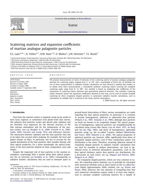
Icarus 199 (2009) 219–230
Contents lists available at ScienceDirect
Icarus
www.elsevier.com/locate/icarus
Scattering matrices and expansion coefficients
of martian analogue palagonite particles
E.C. Laan a,b,∗ ,H.Volten a,1 ,D.M.Stam c,d , O. Muñoz e ,J.W.Hovenier a ,T.L.Roush f
a Astronomical Institute ‘Anton Pannekoek,’ University of Amsterdam, Kruislaan 403, 1098 SJ Amsterdam, The Netherlands
b TNO Science and Industry, Stieltjesweg 1, 2600 AD, Delft, The Netherlands
c SRON Netherlands Institute for Space Research, Sorbonnelaan 2, 3584 CA Utrecht, The Netherlands
d DEOS, Aerospace Engineering, Technical University Delft, Kluyverweg 1, 2629 HS, Delft, The Netherlands
e Instituto de Astrofísica de Andalucía (CSIC), C/ Camino Bajo de Huétor, 50, 18008 Granada, Spain
f NASA Ames Research Center, MS 245-3, Moffett Field, CA 94035-1000, USA
article info abstract
Article history:
Received 22 October 2007
Revised 13 August 2008
Accepted 25 August 2008
Available online 17 September 2008
Keywords:
Polarimetry
Radiative transfer
Mars, atmosphere
Mars, surface
Mars, climate
We present measurements of ratios of elements of the scattering matrix of martian analogue palagonite
particles for scattering angles ranging from 3 ◦ to 174 ◦ and a wavelength of 632.8 nm. To facilitate the
use of these measurements in radiative transfer calculations we have devised a method that enables us
to obtain, from these measurements, a normalized synthetic scattering matrix covering the complete
scattering angle range from 0 ◦ to 180 ◦ . Our method is based on employing the coefficients of the
expansions of scattering matrix elements into generalized spherical functions. The synthetic scattering
matrix elements and/or the expansion coefficients obtained in this way, can be used to include multiple
scattering by these irregularly shaped particles in (polarized) radiative transfer calculations, such as
calculations of sunlight that is scattered in the dusty martian atmosphere.
© 2008 Elsevier Inc. All rights reserved.
1. Introduction
Dust from the martian surface is regularly swept up by winds to
form local, regional, or sometimes even planet-wide dust storms.
The airborne dust particles scatter and absorb solar radiation and
are therefore very important for the thermal structure of the
thin martian atmosphere and for the temperature of the martian
surface (see e.g. Bougher et al., 2006; Gurwell et al., 2005;
Smith, 2004; Gierasch and Goody, 1972, and references therein).
The interaction between radiation and the dust particles thus has
to be taken into account when studying, for example, the local and
global climate on Mars. In particular, one has to account for the
spatial distribution of the dust particles, their number density, and
their optical properties. For a given wavelength, the optical properties
of the dust particles depend on their composition, sizes and
shapes.
Despite the important role of dust particles in the martian atmosphere,
surprisingly little is known about their optical properties
(for an overview, see Korablev et al., 2005). Consequently, in
radiative transfer calculations that are used to interpret space or
*
Corresponding author at: TNO Science & Industry, Stieltjesweg 1, P.O. Box 155,
2600 AD, Delft, The Netherlands.
E-mail address: erik.laan@tno.nl (E.C. Laan).
1 Currently working at the National Institute for Public Health and the Environment
(RIVM), P.O. Box 1, 3720 BA Bilthoven, The Netherlands.
ground-based observations of Mars, various assumptions are made
regarding the dust optical properties. In particular, it is common
to assume homogeneous, spherical or spheroidal dust particles
(Pollack et al., 1995; Tomasko et al., 1999), although dust particles
on Earth are known to be irregularly shaped. The optical properties
of homogeneous, spherical particles can straightforwardly be
calculated using Lorenz–Mie theory (van de Hulst, 1957; de Rooij
and van der Stap, 1984), and those of homogeneous, spheroidal
particles using e.g. the so-called T-matrix method (Mishchenko
and Travis, 1994; Dubovik et al., 2006). The optical properties of
spherical particles can, however, differ significantly from those of
irregularly shaped particles, even if their composition and/or size
distribution is the same. Therefore, assuming spherical instead of
irregularly shaped particles in radiative transfer calculations that
are used for example to analyze observations, can lead to significant
errors in retrieved atmospheric parameters, such as the
dust optical thickness and/or dust particle size distributions (for
a discussion on such errors, see e.g. Dlugach and Petrova, 2003;
Dlugach et al., 2002).
For irregularly shaped particles, which are very common in nature,
the scattering matrix elements can in principle be calculated
with numerical methods such as those based on the so-called Discrete
Dipole Approximation (DDA) method (see e.g. Draine and
Flatau, 1994). However, the vast amounts of computing time that
such numerical calculations require make it at least very impractical
to calculate complete scattering matrices for a sample of
0019-1035/$ – see front matter © 2008 Elsevier Inc. All rights reserved.
doi:10.1016/j.icarus.2008.08.011

220 E.C. Laan et al. / Icarus 199 (2009) 219–230
particles with various (irregular) shapes and various sizes, in particular
if the particles are large compared to the wavelength of
the scattered light. Alternatively, employing geometrical optics for
unrealistically spiky particles combined with an imaginary part of
the refractive index that is rather small compared to the typical
values used in the literature, appears to be useful to reproduce
the scattering behavior of irregularly shaped mineral particles (see
Nousiainen et al., 2003). As suggested by e.g. Tomasko et al. (1999),
Dlugach and Petrova (2003), Wolff and Clancy (2003), amorepractical
method to obtain elements of the scattering matrix for an ensemble
of irregularly shaped particles is to measure the elements
in a laboratory. Note that measured scattering matrix elements are
also essential for validating numerical methods and approximations.
In this article, we present measurements of ratios of elements
of the scattering matrix of irregularly shaped, randomly oriented
martian analogue palagonite particles, described by Banin et al.
(1997), as functions of the scattering angle. The material palagonite
is believed to be a reasonable, but not perfect, analogue for the
martian surface and atmospheric dust particles. Terrestrial palagonite
particles (i.e. terrestrial weathering products of basaltic ash or
glass) have been put forward as martian dust analogues (Evans and
Adams, 1981; Roush and Bell, 1995) because of spectral similarities
observed with visible and near-infrared spectroscopic observations
using both Earth-based telescopes and several Mars orbiting spacecraft
(Singer, 1985; Soderblom, 1992).
The measurements have been performed using a HeNe laser,
which has a wavelength of 632.8 nm, and for scattering angles, Θ,
ranging from 3 ◦ (near-forward scattering) to 174 ◦ (near-backward
scattering). Other examples of such measurements for irregularly
shaped mineral particles obtained with the same experimental setup
have been reported by e.g. Volten et al. (2005) and references
therein. Since we have measured ratios of all (non-zero) elements
of the scattering matrix as functions of the scattering angle, our
results can be used for radiative transfer calculations that include
multiple scattering and polarization. As described by e.g. Lacis et
al. (1998), ignoring polarization, i.e. using only scattering matrix
element (1, 1) (the so-called phase function), in multiple scattering
calculations, induces errors in calculated fluxes. The use of only the
phase function should be limited to single scattering calculations
for unpolarized incident light.
A practical limitation of our experimental method is that we
cannot measure close (

Scattering matrices of martian analogue palagonite 221
Fig. 1. Scanning electron microscope (SEM) image of the martian analogue palagonite particles used in this study. Note that SEM images generally give a good indication of
the typical shapes of particles, but not necessarily of their sizes.
Fig. 2. Measured size distributions of the martian analogue palagonite particles.
The lines refer to the normalized number distribution (plusses), the normalized
projected-surface-area distribution (triangles), and the normalized volume distribution
(crosses) as functions of log r, withr the radius (in microns) of a projectedsurface-area-equivalent
sphere (see Volten et al., 2005, for the definitions of the
various distributions). Approximating the normalized number distribution with a
log normal distribution function yields r eff = 4.46 μm and v eff = 7.29.
We are well aware of the fact that the sizes of real martian dust
particles can be very different from those in our sample. Indeed,
sizes of dust particles on Mars will probably vary from location to
location, and from time to time, especially when in local or global
storms, dust particles are lifted up from the surface to be deposited
somewhere else: depending on the atmospheric turbulence, the
particles in the martian atmosphere could have very different size
distributions than those on the surface.
The effective radius of 4.46 μm of our sample particles is a factor
of 2 to 3 larger than the values put forward for the effective radius
of martian dust by Wolff and Clancy (2003), who analyzed observations
by the Thermal Emission Spectrometer (TES) on-board
the Mars Global Surveyor, and by Pollack et al. (1995), who analyzed
observations performed by the Viking Lander. In particular,
Pollack et al. (1995) derived an effective radius of 1.85 ± 0.3 μm.
From Pathfinder measurements, Tomasko et al. (1999) derived an
effective radius of 1.6±0.15 μm. Lemmon et al. (2004) derived values
from observations by the Mars Exploration Rovers Spirit and
Opportunity that are similar to those of Pollack et al. (1995) and
Tomasko et al. (1999).
Although our sample particles thus seem to be rather large,
it should be noted that particle sizes as derived from observations
will depend on the observing method, e.g. looking at diffuse
skylight or at the surface, as well as on the retrieval method. In
particular, according to numerical simulations by Dlugach et al.
(2002), effective radii that are derived for spheroidal dust particles
at visible wavelengths, under the assumption that these particles
are spherical, can be significantly underestimated. At infrared
wavelengths, Min et al. (2003) and Fabian et al. (2001) show that
absorption and emission processes, even in the small size parameter
regime (i.e. 2πr eff /λ 1), depend on the particle shape, too.
Clearly, because martian dust is expected to show a great variety
in microphysical properties, our results should simply be regarded
as an example of what can be expected for the scattering properties
of irregularly shaped particles.
3. The scattering matrix
3.1. Definition of the scattering matrix
The flux and state of polarization of a quasi-monochromatic
beam of light can be described by means of a so-called flux vector.
If such a beam of light is scattered by an ensemble of randomly
oriented particles, separated by distances larger than their linear
dimensions and in the absence of multiple scattering as in our experimental
set-up (see Section 3.2), the flux vectors of the incident
beam, π 0 (λ), and scattered beam, π(λ, Θ), areforeachscat-

222 E.C. Laan et al. / Icarus 199 (2009) 219–230
tering direction, related by a 4 × 4 matrix, as follows (van de Hulst,
1957; Volten et al., 2006):
⎛
F 11 F 12 F 13 F 14
(λ, Θ) =
λ2
⎜
F 12 F 22 F 23 F 24
⎟
4π 2 D 2 ⎝ −F 13 −F 23 F 33 F 34
⎠ 0(λ), (1)
F 14 F 24 −F 34 F 44
⎞
where the first elements of the column vectors are fluxes divided
by π and the other elements describe the state of polarization of
the beams by means of Stokes parameters. Furthermore, λ is the
wavelength, and D is the distance between the ensemble of particles
and the detector. The scattering plane, i.e. the plane containing
the directions of the incident and scattered beams, is the plane of
reference for the flux vectors. The matrix, F, withelementsF ij is
called the scattering matrix of the ensemble. The scattering matrix
elements F ij are dimensionless, and depend on the number of
the particles and on their microphysical properties (size, shape and
refractive index), the wavelength of the light, and the scattering direction.
For randomly oriented particles, the scattering direction is
fully described by the scattering angle Θ, the angle between the
directions of propagation of the incident and the scattered beams.
According to Eq. (1), a scattering matrix has in general 10 different
matrix elements. For randomly oriented particles with equal
amounts of particles and their mirror particles, as we can assume
applies for the particles of our ensemble, the four elements
F 13 (Θ), F 14 (Θ), F 23 (Θ), and F 24 (Θ) are zero over the entire scattering
angle range (see van de Hulst, 1957). This leaves us only six
non-zero scattering matrix elements, as follows
⎡
F 11 (Θ) F 12 (Θ)
⎤
0 0
F(Θ) = ⎢
F 12 (Θ) F 22 (Θ) 0 0
⎥
⎣ 0 0 F 33 (Θ) F 34 (Θ) ⎦ , (2)
0 0 −F 34 (Θ) F 44 (Θ)
where |F ij (Θ)/F 11 (Θ)| 1(Hovenier et al., 1986).
For unpolarized incident light, matrix element F 11 (Θ) is proportional
to the flux of the singly scattered light and is also called
the phase function. Also, for unpolarized incident light, the ratio
−F 12 (Θ)/F 11 (Θ) equals the degree of linear polarization of the
scattered light. The sign indicates the direction of polarization: a
negative degree of polarization indicates that the scattered light is
polarized parallel to the reference plane, whereas a positive degree
of polarization indicates that the light is polarized perpendicular to
the reference plane. In calculations for fluxes only and where light
is scattered only once, F 11 (Θ) is the only matrix element that is
required. Ignoring the other matrix elements, and hence the state
of polarization of the light, in multiple scattering calculations, usually
leads to errors in calculated fluxes (see e.g. Lacis et al., 1998;
Moreno et al., 2002; Stam and Hovenier, 2005).
3.2. The experimental set-up
Our measurements have been performed with the light scattering
experiment located in Amsterdam, the Netherlands (see
e.g. Volten et al., 2005; Hovenier et al., 2003; Hovenier, 2000;
Volten et al., 2001; Muñoz et al., 2000). Fig. 3 shows a sketch of
the experimental set-up. In our experimental apparatus, we use a
HeNe laser (λ = 632.8 nm, 5 mW) as a light source. The laser light
passes through a polarizer and an electro-optic modulator. The
modulated light is subsequently scattered by an ensemble of randomly
oriented particles from the sample, located in a jet stream
produced by an aerosol generator. The scattered light may pass
through a quarter-wave plate and an analyzer, depending on the
scattering matrix element of interest (for details see e.g. Volten et
al., 2005), and is then detected by a photomultiplier tube which
moves in steps along a ring with radius D (see Eq. (1)) aroundthe
Fig. 3. Sketch of the experimental set-up. The light source (a HeNe laser) emits a
beam of quasi-monochromatic light, which passes through a polarizer and a modulator
(not shown). The light is scattered by the ensemble of palagonite particles.
A detector measures the flux that is scattered over a scattering angle Θ. Measurements
can be performed for 3 ◦ Θ 174 ◦ .
ensemble of particles; in this way a range of scattering angles from
3 ◦ (nearly forward scattering) to 174 ◦ (nearly backward scattering)
is covered in the measurements.
We cannot measure close (

Scattering matrices of martian analogue palagonite 223
Fig. 4. Ratios of scattering matrix elements as functions of the scattering angle. Crosses show the ratios of elements measured, at λ = 632.8 nm, for the martian analogue
palagonite particles, with the vertical bars indicating the experimental errors. Solid lines show the ratios of elements calculated using Mie-theory for homogeneous, spherical
particles that are distributed in size as shown in Fig. 2.
smallest scattering angles (the so-called forward scattering peak)
and a smooth drop-off towards the largest scattering angles. The
measured phase function is very flat for scattering over intermediate
(70 ◦

224 E.C. Laan et al. / Icarus 199 (2009) 219–230
F 44 (Θ) (Hovenier et al., 2004), whereas we find significant differences
where C is a normalization constant. This constant can in principle
where dω is an element of solid angle. Combining Eq. (4) and thetic matrix elements F au (Θ) for i, j = 1 to 4 with the exception
of i = j = 1 from the measured ratios F ij (Θ)/F 11 (Θ), using
Eq. (5) and setting F au
ij
11 (30◦ ) equal to 1/C leads to
∫
Eq. (3). To obtain also the complete scattering angle range for the
1 F 11 (Θ)
4π F 11 (30 ◦ ) dω = C. (6) other scattering matrix element ratios, we extrapolate the measured
F
4π
ij (Θ)/F 11 (Θ) (i, j = 1 to 4 with the exception of i = j = 1)
between the measured F 44 (Θ)/F 11 (Θ) and F 33 (Θ)/F 11 (Θ)
for the palagonite sample. The ratio F 33 (Θ)/F 11 (Θ) is zero at a
smaller scattering angle than F 44 (Θ)/F 11 (Θ), and has a lower
minimum (−0.5 versus −0.2). Indeed, for the irregularly shaped
particles, these ratios show an apparently typical behavior for nonspherical
particles (Mishchenko et al., 2000), namely, at large scattering
angles, F 44 (Θ)/F 11 (Θ) is larger than F 33 (Θ)/F 11 (Θ).
Finally, scattering matrix element ratio F 34 (Θ)/F 11 (Θ) of the
irregularly shaped particles shows a shallow bell shape with
be obtained by evaluating the integral on the left-hand side of
Eq. (6), provided the function to be integrated is known over the
full range of scattering angles. Therefore, we added artificial datapoints
at 0 ◦ and 180 ◦ tothemeasuredvaluesofF 11 (Θ)/F 11 (30 ◦ ).
At Θ = 180 ◦ , the smoothness of the measured phase function allows
us to simply add an artificial data point to F 11 (Θ)/F 11 (30 ◦ )
by spline extrapolation (Press et al., 1992) of the measured data
points.
Adding an artificial data point to the measured F 11 (Θ)/F 11 (30 ◦ )
slightly negative branches for Θ165 ◦ . This at Θ = 0 ◦ , is more complicated. Numerical tests with the calculated
scattering angle dependence is commonly found for irregularly
shaped silicate particles (e.g. Volten et al., 2001, 2005; Muñoz et
al., 2000). Interestingly, whereas for the irregularly shaped particles,
F 34 (Θ)/F 11 (Θ) is very similar to −F 12 (Θ)/F 11 (Θ), for the
spherical particles, these ratios differ strongly from each other,
phase function for the hypothetical homogeneous, spher-
ical palagonite particles (see Fig. 4) show that extrapolation of
the calculated phase function at Θ 3 ◦ towards Θ = 0 ◦ , using
e.g. splines (Press et al., 1992), fails to reproduce the strength of
the calculated forward scattering peak. We thus decided not to
both in sign and in shape, as can be seen in Fig. 4.
extrapolate the measured phase function from Θ = 3 ◦ towards
Comparison between the measured and the calculated scattering
matrix element ratios in Fig. 4 supports the idea that scattering
by non-spherical particles generally leads to smoother functions
of the scattering angle than scattering by spherical particles. This
smooth scattering behavior by irregularly shaped particles proves
to be very difficult to simulate numerically without taking into account
the irregular shape of the particles (Nousiainen et al., 2003;
Nousiainen and Vermeulen, 2003; Kokhanovsky, 2003).
An electronic table of the measured ratios of the elements of
the scattering matrix will be available from the Amsterdam Light
Scattering Database (Volten et al., 2005, 2006).
Θ = 0 ◦ . Instead we add an artificial data point to the measured
F 11 (Θ)/F 11 (30 ◦ ) at Θ = 0 ◦ using the phase function that we calculated
for the projected-surface-area equivalent, homogeneous,
spherical particles. The rationale for this approach, which is similar
to that used by Liu et al. (2003) and Muñoz et al. (2007), is
that the forward scattering peak results mainly from the diffraction
of the incident light. The strength of the diffraction peak
and its scattering angle dependence appears to depend mainly
on the size of the particles and fairly shape independent for
projected-surface-area equivalent convex particles in random orientation
(Mishchenko et al., 2002).
Because our normalization of the measured phase function,
3.4. The auxiliary scattering matrix
F 11 (Θ)/F 11 (30 ◦ ), atΘ = 30 ◦ is rather arbitrary (we could have
chosen a different value of Θ for the normalization), we scale the
It appears to be difficult to directly use the measured ratios
of elements of the scattering matrix in radiative transfer calculations,
because of the lack of measurements below Θ = 3 ◦ and
phase function as calculated for the spherical palagonite particles
to the measured phase function. For this, we use the following
equation,
above Θ = 174 ◦ . In particular, it would be interesting to have the
forward scattering peak in the phase function since it contains a F 11 (0 ◦ )
large fraction of the scattered energy (see Fig. 4), and is thus very F 11 (30 ◦ ) = F s 11 (0◦ ) F 11 (3 ◦ )
F s 11 (3◦ ) F 11 (30 ◦ ) , (7)
important for the accurate modeling of scattered light in e.g. planetary
atmospheres. In addition, the lack of measurements at small
11 (0 ◦ )/F 11 (30 ◦ ) the artificial data point at Θ = 0 ◦ and the
with F
superscript “s” indicating the phase function as calculated for the
and large scattering angles inhibits the normalization of scattering
matrix elements such that the average of the phase function
spherical particles.
over all scattering directions equals unity. With such a normalization
and a value for the single scattering albedo of the scattering
We now have data points available across the full scattering
angle range to evaluate the integral in Eq. (6) and to obtain
the normalization constant C. The numerical evaluation of
particles, one could model the absolute amount of radiation that is
scattered in a given direction.
this integral, however, appears to be difficult because of the
To facilitate the use of the measured ratios of elements of the
steep slope between Θ = 0 ◦ and Θ = 3 ◦ , where no measured
scattering matrix in radiative transfer calculations, we construct
data points are available. Therefore, we have chosen a different
from these a so-called auxiliary scattering matrix, F au , for which
method to obtain the normalization constant C in Eq. (6). This
holds (for i, j = 1 to 4 with the exception of i = j = 1)
method is based on the expansion of the measured phase function
F 11 (Θ)/F 11 (30 ◦ ), including the added, artificial, data points
F au
ij (Θ) = F ij(Θ)
F 11 (Θ) F au
11
(Θ), (3)
at Θ = 0 ◦ to Θ = 180 ◦ , as a function of the scattering angle
into so-called generalized spherical functions (Gel’fand et al., 1963;
where the auxiliary phase function F au
Hovenier and van der Mee, 1983; de Rooij and van der Stap, 1984;
11 is equal to
Hovenier et al., 2004). This method of obtaining expansion coefficients
from scattering matrix elements is explained in detail in
F au
11 (Θ) = F 11(Θ)
F 11 (30 ◦ ) F au
11 (30◦ ) for 3 ◦ Θ 174 ◦ . (4)
Section 4. The expansion of F 11 (Θ)/F 11 (30 ◦ ) yields expansion coefficients
α l This auxiliary phase function is normalized according to
1 (with 0 l). The first of these expansion coefficients,
∫
α 0 1 , is equal to constant C in Eq. (6) (Hovenier et al., 2004). Having
1
F au
obtained C in this way, and thus F
11
(Θ) dω = 1, (5)
11 (30◦ ),wereadilyfindF au
11 (Θ)
4π
from the measured ratio F 11 (Θ)/F 11 (30 ◦ ) and Eq. (4).
4π
Next, given the auxiliary phase function, we derive the syn-

Scattering matrices of martian analogue palagonite 225
towards Θ = 0 ◦ and 180 ◦ . At these two scattering angles, the following
equalities should hold (see Display 2.1 in Hovenier et al.,
0,0 (cos Θ), (17)
∞∑
a 4 (Θ) = α l 4
l=0
2004):
∞∑
F 12 (0 ◦ )/F 11 (0 ◦ ) = F 34 (0 ◦ )/F 11 (0 ◦ ) = 0, (8)
b 1 (Θ) = β l 1 P l 0,2 (cos Θ), (18)
best approximation in the least-squares sense, both for overdetermined
systems (in which the number of data points is larger
∞∑
a 1 (Θ) = α l 1 P l 0,0 (cos Θ), (14)
than the required number of expansion coefficients) and underdetermined
systems (in which the number of data points is smaller
∞∑ (
l=0
a 2 (Θ) + a 3 (Θ) = α
l
2 + ) αl 3 P
l
2,2 (cos Θ), (15)
than the required number of expansion coefficients).
To test the robustness and the quality of the fit method based
l=2
on the SVD method, we applied it to scattering matrix elements
∞∑ (
a 2 (Θ) − a 3 (Θ) = α
l
2 − ) αl 3 P
l
2,−2 (cos Θ), (16) that we calculated for the hypothetical, spherical palagonite particles,
and that are shown in Fig. 4 (note that our Mie-algorithm
l=2
F 22 (0 ◦ )/F 11 (0 ◦ ) = F 33 (0 ◦ )/F 11 (0 ◦ ), (9)
∞∑
F 22 (180 ◦ )/F 11 (180 ◦ ) =−F 33 (180 ◦ )/F 11 (180 ◦ ), (10)
b 2 (Θ) = β l 2 P l 0,2 (cos Θ). (19)
l=2
F 12 (180 ◦ )/F 11 (180 ◦ ) = F 34 (180 ◦ )/F 11 (180 ◦ ) = 0, (11)
F 44 (180 ◦ )/F 11 (180 ◦ ) = 1 − 2F 22 (180 ◦ )/F 11 (180 ◦ ). (12)
Here, α l 1 , αl 2 , αl 3 , αl 4 , βl 1 , and βl 2 are the expansion coefficients. For
each value of integer l, the expansion coefficients can be derived
Following Eq. (8), ratiosF 12 (0 ◦ )/F 11 (0 ◦ ) and F 34 (0 ◦ )/F 11 (0 ◦ ) are
set equal to zero. Following Eq. (9), we use splines to extrapolate
the ratios F 22 (Θ)/F 11 (Θ) and F 33 (Θ)/F 11 (Θ) towards Θ = 0 ◦ ,
and we set both F 22 (0 ◦ )/F 11 (0 ◦ ) and F 33 (0 ◦ )/F 11 (0 ◦ ) equal to the
average of the two extrapolated values. Ratio F 44 (0 ◦ )/F 11 (0 ◦ ) is
from the auxiliary scattering matrix elements using the definitions
of the generalized spherical functions and their orthogonality relations
(see Hovenier et al., 2004).
A similar expansion in generalized spherical functions can be
made for any scattering matrix of the form given by Eq. (2). The
obtained by extrapolating (with splines) the ratio F 44 (Θ)/F 11 (Θ) coefficient α 0 1 is always equal to the average of the one–one element
over all directions (Hovenier et al., 2004). So for the auxiliary
from Θ = 3 ◦ towards Θ = 0 ◦ .
In the backward scattering direction, the measured scattering phase function a 1 (Θ) we have, according to Eq. (5), α 0 1
= 1 and for
matrix element ratios F ij (Θ)/F 11 (Θ) appear to be smooth functions
of Θ (see Fig. 4). We use splines (Press et al., 1992) to extrapolate
the measured phase function, F 11 (Θ)/F 11 (30 ◦ ) we have α 0 1
= C, as
mentioned in Section 3.4.
F 22 (Θ)/F 11 (Θ), and F 33 (Θ)/F 11 (Θ) from Θ = 174 ◦ to Θ =
180 ◦ .BecauseF 22 (180 ◦ )/F 11 (180 ◦ ) should be equal to −F 33 (180 ◦ )/ 4.2. The singular value decomposition method
F 11 (180 ◦ ) (see Eq. (10)), we set both F 22 (180 ◦ )/F 11 (180 ◦ ) and
−F 33 (180 ◦ )/F 11 (180 ◦ ) equal to the average of the two extrapolated
To derive the expansion coefficients of the measured phase
values. Following Eq. (11), we set F 12 (180 ◦ )/F 11 (180 ◦ ) function, including the points added at 0 ◦ and 180 ◦ , and of all six
and F 34 (180 ◦ )/F 11 (180 ◦ ) equal to zero, and calculate F 44 (180 ◦ )/
F 11 (180 ◦ ) using Eq. (12) with F 22 (180 ◦ )/F 11 (180 ◦ ).
elements of the auxiliary scattering matrix we write each of the
Eqs. (14)–(19) into the following general form:
In the following, we will refer to the elements of our auxiliary
m∑
scattering matrix F au (Θ) as (see Hovenier et al., 2004):
y(Θ) = γ l X l (Θ),
⎡
a 1 (Θ) b 1 (Θ)
⎤
0 0
l=n
(20)
F au (Θ) = ⎢
b 1 (Θ) a 2 (Θ) 0 0
⎥
⎣ 0 0 a 3 (Θ) b 2 (Θ) ⎦ . (13) where y(Θ) represents the value of the measured phase function
or an auxiliary scattering matrix element at scattering angle
0 0 −b 2 (Θ) a 4 (Θ)
Θ, or, in the case of a 2 and a 3 , respectively their sum, as
in Eq. (15), or difference, as in Eq. (16). The functions X l (Θ) in
4. Expansion coefficients
Eq. (20) are the basis functions, for which we choose the appropriate
generalized spherical functions (Hovenier et al., 2004;
4.1. Definitions of the expansion coefficients
de Haan et al., 1987). The parameters γ l in Eq. (20) represent
the expansion coefficients, or, in the case of α l 2 and αl 3 , respectively
their sum (Eq. (15)) ordifference(Eq.(16)). Furthermore in
For use in numerical radiative transfer algorithms, it is often advantageous
to expand the elements of a scattering matrix as functions
of the scattering angle into so-called generalized spherical
functions (Gel’fand et al., 1963; Hovenier and van der Mee, 1983;
de Rooij and van der Stap, 1984; Hovenier et al., 2004). The
advantage of using the coefficients of this expansion, the socalled
expansion coefficients, instead of the elements of a scattering
matrix themselves is that it can significantly speed up
Eq. (20), n equals 0 or 2, depending on the auxiliary scattering
matrix element under consideration (see Eqs. (14)–(19)), and, although
theoretically m equals ∞ (see Eqs. (14)–(19)), in practice m
is restricted to the number of scattering angles at which values of
the auxiliary scattering matrix elements y(Θ) are available.
For a linear model such as that represented by Eq. (20), the
merit function χ 2 is generally defined as
multiple scattering calculations, which is of particular importance
when polarization is taken into account (Hovenier et al., 2004;
k∑
[
χ 2 y(Θi ) − ∑ m
l=n
=
X l ] 2
(Θ i )
, (21)
de Haan et al., 1987).
σ i
We indicate the generalized spherical functions by Pm,n l i=1
(cos Θ)
with the indices m and n equal to +2, +0, −0, or −2, and with where k is the number of available data points and σ i is the error
l max{|m|, |n|}. Note that generalized spherical function P l 0,0 is
simply a Legendre polynomial. The expansion of the elements of
auxiliary scattering matrix F au (Θ) (see Eq. (13)) into generalized
spherical functions is as follows:
associated with data point y(Θ i ). We use the Singular Value Decomposition
(SVD) method (Press et al., 1992) tosolveEq.(21) for
the expansion coefficients γ l , because this method is only slightly
susceptible to roundoff errors and provides a solution that is the
l=2

226 E.C. Laan et al. / Icarus 199 (2009) 219–230
Fig. 5. The expansion coefficients α l 1 , αl 2 , αl 3 , αl 4 , βl 1 and βl 2 as functions of integer l, with their absolute errors, as derived from the auxiliary scattering matrix elements
a 1 (Θ), a 2 (Θ), a 3 (Θ), a 4 (Θ), b 1 (Θ), andb 2 (Θ), respectively.
(de Rooij and van der Stap, 1984) provides matrix elements normalized
according to Eq. (5), althoughinFig. 4, the normalization
of the elements has been adapted to correspond to that of the
measurements). For the test we compare the matrix elements calculated
with our Mie-algorithm with the matrix elements obtained
using the expansion coefficients derived with the SVD method and
Eqs. (14)–(19). For the relative errors in the matrix elements we
adopt the values of the experimental errors.
We tested two aspects of the application of the SVD method.
First, we applied the method to matrix elements calculated at the
same set of scattering angles as the measured ratios of matrix elements,
i.e. having a typical angular resolution of 5 ◦ and scattering
angles ranging from 3 ◦ to 174 ◦ . Comparing the matrix elements
obtained using the expansion coefficients that were derived with
the SVD method with the directly calculated matrix elements, we
found that the relatively coarse angular sampling and the lack of
data points below Θ = 3 ◦ gave rise to strong oscillations in the
matrix elements that were calculated from the derived expansion
coefficients. In addition, with the derived expansion coefficients,
we could not reproduce the strong forward scattering peak in the
phase function. The lack of data points above Θ = 174 ◦ appeared
to be less of a problem, probably because of the smoothness of the
matrix elements at those scattering angles.
Second, we applied the SVD method to matrix elements calculated
at an angular resolution of 1 ◦ and covering the full scattering
angle range, i.e. from 0 ◦ to 180 ◦ . The matrix elements obtained
using the hence derived expansion coefficients coincided within
the numerical precision with the directly calculated matrix elements.
From this we conclude that our implementation of the SVD
method is reliable, but that we have to apply it to the whole scattering
angle range, and with a relatively high angular resolution.
Finally, we found that averaging two sets of derived expansion
coefficients, one of which has one coefficient more than the other,
removes most of the left-over oscillations in the scattering matrix
element that is calculated with the coefficients.
4.3. The derived expansion coefficients
For deriving the expansion coefficients of the scattering matrix
elements of the martian analogue palagonite particles, we use
the elements of the auxiliary scattering matrix F au (Θ) (see Section
3.4), because they cover the whole scattering angle range and
are normalized according to Eq. (5).
We increase the angular sampling of the auxiliary scattering
matrix by adding artificial data points by spline interpolation to
the dataset between Θ = 3 ◦ and 174 ◦ . Starting with 44 measured
data points per matrix element, adding the artificial data points results
in 220 data points for each of the auxiliary scattering matrix
elements. This amount of artificial data points includes the values
at the forward and backward scattering angles at respectively
Θ = 0 ◦ and Θ = 180 ◦ as described in Section 3.4. The 220 datapoints
proved to be required to be able to follow the steep slopes
of a 1 (Θ), a 2 (Θ), a 3 (Θ) and a 4 (Θ) between Θ = 0 ◦ and Θ = 3 ◦ ,
where no artificial datapoints were added, without introducing unwanted
oscillations. As 220 datapoints are needed to obtain the
auxiliary phase function a 1 (Θ), it proved to be practical to extend
also F 12 (Θ)/F 11 (Θ) and F 34 (Θ)/F 11 (Θ) to the same amount of
220 datapoints, to be able to straightforwardly apply Eq. (3) to obtain
b 1 (Θ) and b 2 (Θ).
The optimal number of expansion coefficients for each of the
elements was obtained in an iterative process: unrealistic oscillations
at large scattering angles are suppressed when using a
smaller number of expansion coefficients, while the fit of the steep

Scattering matrices of martian analogue palagonite 227
Fig. 6. The synthetic scattering matrix elements a 1 , a 2 , a 3 , a 4 , b 1 ,andb 2 as functions of the scattering angle Θ.
phase function near 0 ◦ is improved when using a larger number
of expansion coefficients. Applying our SVD method to the auxiliary
scattering matrix elements, leaves us with respectively 185
expansion coefficients for a 1 (Θ), a 2 (Θ), a 3 (Θ), a 4 (Θ), 130 expansion
coefficients for b 1 (Θ) and 46 expansion coefficients for b 2 (Θ).
Fig. 5 shows the expansion coefficients α l 1 , αl 2 , αl 3 , αl 4 , βl 1 , and βl 2 ,
derived from the auxiliary scattering matrix of the martian analogue
palagonite particles. The expansion coefficients are plotted
with error bars that originate from the experimental errors in the
measurements. An electronic table of the expansion coefficients
will be available from the Amsterdam Light Scattering Database 3
(Volten et al., 2005, 2006).
4.4. The synthetic scattering matrix
Employing Eqs. (14)–(19) with the expansion coefficients presented
in Section 4.3, we can now calculate, at an arbitrary angular
resolution, the so-called synthetic scattering matrix (see also Muñoz
et al., 2004) which covers the complete scattering range, i.e. from
0 ◦ to 180 ◦ , and which is normalized according to Eq. (5). Fig. 6
shows the calculated synthetic scattering matrix elements. The elements
of the synthetic scattering matrix are also listed in Table 1
at an angular resolution of 1 ◦ to 5 ◦ . An electronic table of the
synthetic scattering matrix elements will be available from the
Amsterdam Light Scattering Database (Volten et al., 2005, 2006).
As a check we used the synthetic scattering matrix to compute the
same ratios of elements as have been measured. We found the differences
to lie within the ranges of experimental uncertainties or
very nearly so.
3 Website: http://www.astro.uva.nl/scatter.
5. Summary and discussion
We present measured ratios of elements of the scattering matrix
of irregularly shaped martian analogue palagonite particles
(Roush and Bell, 1995; Banin et al., 1997) as functions of the scattering
angle Θ (3 ◦ Θ 174 ◦ ) at a wavelength of 632.8 nm.
Our measured ratios of scattering matrix elements differ strongly
from those calculated for homogeneous, spherical particles with
the same size and refractive index. In particular, the measured
phase function (ratio F 11 (Θ)/F 11 (30 ◦ )) shows a very strong (almost
three orders of magnitude) forward scattering peak and a
smooth drop-off towards the largest scattering angles, where the
phase function of the spherical particles shows much more angular
features especially in the backward scattering direction. Clearly,
using scattering matrix elements that have been calculated for homogeneous,
spherical particles when irregularly shaped particles
are to be expected in radiative transfer calculations for e.g. the interpretation
of remote-sensing observations can thus lead to errors
in retrieved dust properties (microphysical parameters and/or optical
thicknesses).
To facilitate the use of our measurements in radiative transfer
calculations for e.g. Mars, we have first constructed an auxiliary
scattering matrix from the measured scattering matrix. This auxiliary
scattering matrix covers the whole scattering angle range
(i.e. from 0 ◦ to 180 ◦ ), and its elements have been normalized such
that the average of the phase function over all scattering directions
equals unity. The value of the phase function at Θ = 0 ◦ has been
computed from the phase function calculated with Mie-theory for
homogeneous, spherical particles with the same size and composition.
The normalization of the auxiliary phase function, and
hence the normalization of the other elements too, is obtained by
applying a Singular Value Decomposition (SVD) method to fit an
expansion in generalized spherical functions (Gel’fand et al., 1963;

228 E.C. Laan et al. / Icarus 199 (2009) 219–230
Table 1
The synthetic scattering matrix elements of the martian analogue palagonite particles (Roush and Bell, 1995), as functions of the scattering angle Θ (in degrees). The
scattering angles are identical to those used in the measurements, extended with Θ = 0 ◦ , 1 ◦ , 2 ◦ and from 175 ◦ to 180 ◦ . An electronic version of this table will be available
from the Amsterdam Light Scattering Database (Volten et al., 2005), at http://www.astro.uva.nl/scatter.
Θ a 1 (Θ) a 2 (Θ) a 3 (Θ) a 4 (Θ) b 1 (Θ) b 2 (Θ)
0 4.36E+003 4.26E+003 4.26E+003 4.12E+003 0.00E+000 0.00E+000
1 2.82E+003 2.75E+003 2.75E+003 2.66E+003 −2.34E−003 −7.15E−003
2 6.60E+002 6.43E+002 6.43E+002 6.17E+002 1.98E−002 −2.68E−002
3 3.71E+001 3.58E+001 3.62E+001 3.49E+001 7.32E−002 −5.39E−002
4 2.51E+001 2.43E+001 2.46E+001 2.38E+001 9.69E−002 −8.20E−002
5 1.53E+001 1.46E+001 1.49E+001 1.43E+001 7.28E−002 −1.05E−001
6 1.17E+001 1.13E+001 1.14E+001 1.10E+001 4.88E−002 −1.18E−001
7 8.75E+000 8.44E+000 8.49E+000 8.18E+000 3.73E−002 −1.20E−001
8 7.08E+000 6.82E+000 6.82E+000 6.60E+000 1.66E−002 −1.12E−001
9 5.68E+000 5.48E+000 5.48E+000 5.29E+000 −1.68E−003 −9.83E−002
10 4.80E+000 4.62E+000 4.61E+000 4.42E+000 −1.55E−003 −8.22E−002
15 2.35E+000 2.22E+000 2.21E+000 2.12E+000 −4.94E−003 −4.04E−002
20 1.42E+000 1.32E+000 1.31E+000 1.23E+000 −8.44E−003 −2.15E−002
25 9.68E−001 8.93E−001 8.80E−001 8.13E−001 −9.63E−003 −1.35E−002
30 6.98E−001 6.27E−001 6.18E−001 5.60E−001 −1.05E−002 −3.85E−003
35 5.22E−001 4.57E−001 4.47E−001 4.08E−001 −1.15E−002 2.72E−003
40 4.06E−001 3.44E−001 3.32E−001 3.00E−001 −1.30E−002 8.12E−003
45 3.24E−001 2.68E−001 2.50E−001 2.25E−001 −1.46E−002 9.34E−003
50 2.68E−001 2.13E−001 1.96E−001 1.75E−001 −1.55E−002 1.23E−002
55 2.24E−001 1.71E−001 1.52E−001 1.38E−001 −1.66E−002 1.46E−002
60 1.90E−001 1.37E−001 1.20E−001 1.10E−001 −1.67E−002 1.57E−002
65 1.68E−001 1.15E−001 9.64E−002 8.91E−002 −1.76E−002 1.59E−002
70 1.49E−001 9.70E−002 7.72E−002 7.20E−002 −1.74E−002 1.80E−002
75 1.34E−001 8.14E−002 5.95E−002 5.79E−002 −1.71E−002 1.79E−002
80 1.21E−001 6.99E−002 4.60E−002 4.70E−002 −1.68E−002 1.82E−002
85 1.12E−001 6.03E−002 3.58E−002 3.79E−002 −1.62E−002 1.85E−002
90 1.05E−001 5.30E−002 2.48E−002 3.12E−002 −1.66E−002 1.77E−002
95 9.87E−002 4.73E−002 1.86E−002 2.50E−002 −1.52E−002 1.71E−002
100 9.29E−002 4.19E−002 1.16E−002 2.00E−002 −1.47E−002 1.55E−002
105 8.94E−002 3.81E−002 4.11E−003 1.57E−002 −1.34E−002 1.40E−002
110 8.46E−002 3.42E−002 −9.87E−004 1.16E−002 −1.20E−002 1.35E−002
115 8.10E−002 3.25E−002 −6.60E−003 7.86E−003 −1.19E−002 1.22E−002
120 7.90E−002 3.06E−002 −1.12E−002 4.75E−003 −1.07E−002 1.05E−002
125 7.68E−002 2.86E−002 −1.46E−002 1.22E−003 −8.74E−003 9.90E−003
130 7.34E−002 2.75E−002 −1.77E−002 −8.03E−004 −7.27E−003 8.21E−003
135 7.34E−002 2.77E−002 −2.09E−002 −3.23E−003 −6.32E−003 6.43E−003
140 7.34E−002 2.81E−002 −2.39E−002 −5.64E−003 −4.64E−003 5.94E−003
145 7.41E−002 2.87E−002 −2.62E−002 −7.85E−003 −3.46E−003 5.51E−003
150 7.33E−002 2.97E−002 −2.80E−002 −9.76E−003 −2.55E−003 3.90E−003
155 7.48E−002 3.13E−002 −3.01E−002 −1.26E−002 −8.35E−004 3.86E−003
160 7.68E−002 3.47E−002 −3.50E−002 −1.38E−002 5.71E−005 1.69E−003
165 7.89E−002 3.62E−002 −3.79E−002 −1.58E−002 1.09E−003 −9.02E−005
170 8.04E−002 3.77E−002 −3.95E−002 −1.74E−002 2.37E−003 −1.02E−003
171 8.32E−002 3.90E−002 −4.17E−002 −1.82E−002 1.96E−003 −1.26E−003
172 8.59E−002 4.07E−002 −4.43E−002 −1.81E−002 1.65E−003 −1.73E−003
173 8.67E−002 4.12E−002 −4.40E−002 −1.87E−002 1.82E−003 −2.31E−003
174 8.59E−002 4.10E−002 −4.65E−002 −1.62E−002 2.12E−003 −2.78E−003
175 8.50E−002 4.16E−002 −4.87E−002 −1.38E−002 2.42E−003 −2.92E−003
176 8.42E−002 4.25E−002 −5.02E−002 −1.31E−002 2.31E−003 −2.60E−003
177 8.35E−002 4.42E−002 −5.07E−002 −1.36E−002 1.85E−003 −1.88E−003
178 8.29E−002 4.59E−002 −5.11E−002 −1.49E−002 1.39E−003 −9.97E−004
179 8.23E−002 4.90E−002 −5.00E−002 −1.70E−002 5.81E−004 −2.76E−004
180 8.18E−002 5.04E−002 −5.04E−002 −1.89E−002 0.00E+000 0.00E+000
Hovenier et al., 2004) to the measured phase function, including
artificial data points. The first expansion coefficient yields the required
normalization constant. After the normalization of the auxiliary
phase function, the SVD method is applied to the auxiliary
scattering matrix and its expansion coefficients are obtained.
With the expansion coefficients, a synthetic scattering matrix
is computed for the complete scattering range. It is normalized so
that the average of its one-one element over all directions equals
unity. The synthetic scattering matrix elements can also straightforwardly
be used in radiative transfer calculations. The need to
include all scattering matrix elements, instead of only the phase
function, is obvious for the interpretation of polarization observations.
However, even for flux calculations, all scattering matrix
elements should be used, because ignoring polarization, i.e. using
only the phase function, in multiple scattering calculations induces
errors in calculated fluxes (e.g. Lacis et al., 1998). The use of only
the phase function should be limited to single scattering calculations
for unpolarized incident light.
Fig. 7 shows a comparison between our synthetic phase function
and two phase functions presented by Tomasko et al. (1999)
as derived from diffuse skylight observations of the Imager for
Mars Pathfinder. Each of the phase functions has its own normalization.
The phase functions of Tomasko et al. (1999) show the
same general angular behavior as our synthetic phase function: a
strong forward scattering peak and a smooth drop-off towards the
largest scattering angles. The forward scattering peak of our phase
function appears to be stronger than the peaks of the phase functions
of Tomasko et al. (1999). This can easily be due to the size
difference of the particles. The dust particles in our sample have
an effective radius that is a factor of 2 to 3 larger than that of
Tomasko et al. (1999) (4.46 μm versus 1.6±0.15 μm). The slopes of
the phase functions in the backward scattering direction are very

Scattering matrices of martian analogue palagonite 229
Fig. 7. The synthetic phase function of the martian analogue palagonite particles compared to the phase function derived by Tomasko et al. (1999) from Mars Pathfinder
results. Each of the curves has its own normalization.
similar, and appear to be typical for (terrestrial) irregularly shaped
mineral particles with moderate refractive indices (see e.g. Volten
et al., 2001; Muñoz et al., 2000, 2001). This smooth slope cannot
be easily anticipated from Mie-theory.
The expansion coefficients, the synthetic scattering matrix elements,
and the measured ratios of elements of the scattering
matrix of the martian analogue palagonite particles will all be
available from the Amsterdam Light Scattering Database (for details,
see Volten et al., 2005, 2006). The Amsterdam Light Scattering
Database contains a collection of measured scattering matrix
element ratios, including information on particle sizes and their
composition, for various types of irregularly shaped particles. The
SVD method presented in this article can straightforwardly be applied
to measured scattering matrix elements of particles other
than the martian analogue palagonite particles.
Acknowledgments
We are grateful to Ben Veihelmann for helping with the SEM
image of Fig. 1. It is a pleasure to thank Martin Konert of the
Vrije Universiteit in Amsterdam for performing the size distribution
measurements and Michiel Min of the University of Amsterdam
for fruitful discussions.
References
Banin, A., Han, F.X., Kan, I., Cicelsky, A., 1997. Acidic volatiles and the Mars soil.
J. Geophys. Res. 102, 13341–13356.
Bougher, S.W., Bell, J.M., Murphy, J.R., Lopez-Valverde, M.A., Withers, P.G., 2006. Polar
warming in the Mars thermosphere: Seasonal variations owing to changing
insolation and dust distributions. Geophys. Res. Lett. 33. L02203.
Clancy, R.T., Lee, S.W., Gladstone, G.R., McMillan, W.W., Rousch, T., 1995. A new
model for Mars atmospheric dust based upon analysis of ultraviolet through
infrared observations from Mariner 9, Viking, and PHOBOS. J. Geophys. Res. 100,
5251–5263.
de Haan, J.F., Bosma, P.B., Hovenier, J.W., 1987. The adding method for multiple scattering
calculations of polarized light. Astron. Astrophys. 183, 371–391.
de Rooij, W.A., van der Stap, C.C.A.H., 1984. Expansion of Mie scattering matrices in
generalized spherical functions. Astron. Astrophys. 131, 237–248.
Dlugach, Z.M., Petrova, E.V., 2003. Polarimetry of Mars in high-transparency periods:
How reliable are the estimates of aerosol optical properties? Solar System
Res. 37, 87–100.
Dlugach, Z.M., Mishchenko, M.I., Morozhenko, A.V., 2002. The effect of the shape
of dust aerosol particles in the martian atmosphere on the particle parameters.
Solar System Res. 36, 367–373.
Draine, B.T., Flatau, P.J., 1994. Discrete-dipole approximation for scattering calculations.
Opt. Soc. Am. J. A 11, 1491–1499.
Dubovik,O.,Sinyuk,A.,Lapyonok,T.,Holben,B.N.,Mishchenko,M.,Yang,P.,Eck,T.F.,
Volten, H., Muñoz, O., Veihelmann, B., van der Zande, W.J., Leon, J.-F., Sorokin,
M., Slutsker, I., 2006. Application of spheroid models to account for aerosol
particle non-sphericity in remote sensing of desert dust. J. Geophys. Res. 111.
D11208.
Evans, D.L., Adams, J.B., 1981. Comparison of spectral reflectance properties of terrestrial
and martian surfaces determined from Landsat and Viking orbiter multispectral
images. Lunar Planet. Sci. XII, 271–273.
Fabian, D., Henning, T., Jäger, C., Mutschke, H., Dorschner, J., Wehrhan, O., 2001.
Steps toward interstellar silicate mineralogy. VI. Dependence of crystalline
olivine IR spectra on iron content and particle shape. Astron. Astrophys. 378,
228–238.
Gel’fand, I.M., Minlos, R.A., Shapiro, Z.Y., 1963. Representations of the Rotation and
Lorentz Groups and Their Applications. Pergamon, New York.
Gierasch, P.J., Goody, R.M., 1972. The effect of dust on the temperature of the martian
atmosphere. J. Atmos. Sci. 29, 400–404.
Gurwell, M.A., Bergin, E.A., Melnick, G.J., Tolls, V., 2005. Mars surface and atmospheric
temperature during the 2001 global dust storm. Icarus 175, 23–31.
Hansen, J.E., Travis, L.D., 1974. Light scattering in planetary atmospheres. Space Sci.
Rev. 16, 527–610.
Herman, M., Deuzé, J.-L., Marchand, A., Roger, B., Lallart, P., 2005. Aerosol remote
sensing from POLDER/ADEOS over the ocean: Improved retrieval using a nonspherical
particle model. J. Geophys. Res. 110 (D9), doi:10.1029/2004JD004798.
D10S02.

230 E.C. Laan et al. / Icarus 199 (2009) 219–230
Hovenier, J.W., 2000. Measuring scattering matrices of small particles at optical
wavelengths. In: Mishchenko, M.I., Hovenier, J.W., Travis, L.D. (Eds.), Light Scattering
by Nonspherical Particles: Theory, Measurements and Applications. Academic
Press, San Diego, pp. 355–365.
Hovenier, J.W., van der Mee, C.V.M., 1983. Fundamental relationships relevant to the
transfer of polarized light in a scattering atmosphere. Astron. Astrophys. 128,
1–16.
Hovenier, J.W., van de Hulst, H.C., van der Mee, C.V.M., 1986. Conditions for the
elements of the scattering matrix. Astron. Astrophys. 157, 301–310.
Hovenier, J.W., van der Mee, C., Domke, H., 2004. Transfer of Polarized Light in
Planetary Atmospheres: Basic Concepts and Practical Methods. Kluwer/Springer,
Dordrecht/Berlin.
Hovenier, J.W., Volten, H., Muñoz, O., van der Zande, W.J., Waters, L.B., 2003. Laboratory
studies of scattering matrices for randomly oriented particles: Potentials,
problems, and perspectives. J. Quant. Spectrosc. Radiat. Trans. 79–80, 741–755.
Kahnert, M., Nousiainen, T., 2007. Variational data-analysis method for combining
laboratory-measured light-scattering phase functions and forward-scattering
computations. J. Quant. Spectrosc. Radiat. Trans. 103, 27–42.
Kokhanovsky, A.A., 2003. Optical properties of irregularly shaped particles. J. Phys.
D Appl. Phys. 36, 915–923.
Konert, M., Vandenberghe, J., 1997. Comparison of laser grain size analysis with
pipette and sieve analysis: A solution for the underestimation of the clay fraction.
Sedimentology 44, 523–535.
Korablev, O., Moroz, V.I., Petrova, E.V., Rodin, A.V., 2005. Optical properties of dust
and the opacity of the martian atmosphere. Adv. Space Res. 35, 21–30.
Lacis, A.A., Chowdhary, J., Mishchenko, M.I., Cairns, B., 1998. Modeling errors in
diffuse-sky radiation: Vector vs scalar treatment. Geophys. Res. Lett. 25, 135–
138.
Lemmon, M.T., Wolff, M.J., Smith, M.D., Clancy, R.T., Banfield, D., Landis, G.A., Ghosh,
A., Smith, P.H., Spanovich, N., Whitney, B., Whelley, P., Greeley, R., Thompson,
S., Bell, J.F., Squyres, S.W., 2004. Atmospheric imaging results from the Mars
exploration rovers: Spirit and opportunity. Science 306, 1753–1756.
Liu, L., Mishchenko, M.I., Hovenier, J.W., Volten, H., Muñoz, O., 2003. Scattering matrix
of quartz aerosols: Comparison and synthesis of laboratory and Lorenz–Mie
results. J. Quant. Spectrosc. Radiat. Trans. 79–80, 911–920.
Min, M., Hovenier, J.W., de Koter, A., 2003. Shape effects in scattering and absorption
by randomly oriented particles small compared to the wavelength. Astron.
Astrophys. 404, 35–46.
Mishchenko, M.I., Hovenier, J., Travis, L., 2000. Light Scattering by Non-spherical
Particles. Theory, Measurements and Applications. Academic Press, San Diego.
Mishchenko, M.I., Travis, L.D., 1994. T-matrix computations of light scattering by
large spheroidal particles. Opt. Commun. 109, 16–21.
Mishchenko, M.I., Travis, L.D., Lacis, A.A., 2002. Scattering, Absorption, and Emission
of Light by Small Particles. Cambridge University Press.
Moreno, F., Muñoz, O., López-Moreno, J.J., Molina, A., Ortiz, J.L., 2002. A Monte Carlo
code to compute energy fluxes in cometary nuclei. Icarus 156, 474–484.
Muñoz, O., Volten, H., de Haan, J.F., Vassen, W., Hovenier, J.W., 2000. Experimental
determination of scattering matrices of olivine and Allende meteorite particles.
Astron. Astrophys. 360, 777–788.
Muñoz, O., Volten, H., de Haan, J.F., Vassen, W., Hovenier, J.W., 2001. Experimental
determination of scattering matrices of randomly oriented fly ash and clay
particles at 442 and 633 nm. J. Geophys. Res. 106, 22833–22844.
Muñoz, O., Volten, H., Hovenier, J.W., Veihelmann, B., van der Zande, W.J., Waters,
L.B.F.M., Rose, W.I., 2004. Scattering matrices of volcanic ash particles of
Mount St. Helens, Redoubt, and Mount Spurr Volcanoes. J. Geophys. Res. 109
(18). D16201.
Muñoz, O., Volten, H., Hovenier, J.W., Nousiainen, T., Muinonen, K., Guirado,
D., Moreno, F., Waters, L.B.F.M., 2007. Scattering matrix of large Saharan
dust particles: Experiments and computations. J. Geophys. Res. 112,
doi:10.1029/2006JD008074. D13215.
Nousiainen, T., Muinonen, K., Räisänen, P., 2003. Scattering of light by large Saharan
dust particles in a modified ray optics approximation. J. Geophys. Res. 108,
doi:10.1029/2001JD001277.
Nousiainen, T., Vermeulen, K., 2003. Comparison of measured single-scattering matrix
of feldspar with T-matrix simulations using spheroids. J. Quant. Spectrosc.
Radiat. Trans. 79–80, 1031–1042.
Pollack, J.B., Ockert-Bell, M.E., Shepard, M.K., 1995. Viking Lander image analysis of
martian atmospheric dust. J. Geophys. Res. 100, 5235–5250.
Press, W.H., Teukolsky, S.A., Vetterling, W.T., Flannery, B.P., 1992. Numerical Recipes
in FORTRAN: The Art of Scientific Computing, second ed. Cambridge University
Press, Cambridge.
Rosenbush, V.K., Kiselev, N.N., 2005. Polarization opposition effect for the Galilean
satellites of Jupiter. Icarus 179, 490–496.
Roush, T.L., Bell, J.F., 1995. Thermal emission measurements 2000-400/cm (5–25 micrometers)
of Hawaiian palagonitic soils and their implications for Mars. J. Geophys.
Res. 100, 5309–5317.
Shkuratov, Y., Kreslavsky, M., Kaydash, V., Videen, G., Bell, J., Wolff, M., Hubbard,
M., Noll, K., Lubenow, A., 2005. Hubble Space Telescope imaging polarimetry of
Mars during the 2003 opposition. Icarus 176, 1–11.
Singer, R.B., 1985. Spectroscopic observation of Mars. Adv. Space Res. 5, 59–68.
Smith, M.D., 2004. Interannual variability in TES atmospheric observations of Mars
during 1999–2003. Icarus 167, 148–165.
Soderblom, L.A., 1992. In: Kieffer, H.H., Jakosky, B.M., Snyder, C.W., Matthews, M.S.
(Eds.), Mars. University of Arizona Press, Tucson.
Stam, D.M., Hovenier, J.W., 2005. Errors in calculated planetary phase functions and
albedos due to neglecting polarization. Astron. Astrophys. 444, 275–286.
Tomasko, M.G., Doose, L.R., Lemmon, M., Smith, P.H., Wegryn, E., 1999. Properties of
dust in the martian atmosphere from the Imager on Mars Pathfinder. J. Geophys.
Res. 104, 8987–9008.
van de Hulst, H.C., 1957. Light Scattering by Small Particles. Wiley, New York.
Veihelmann, B., Volten, H., van der Zande, W.J., 2004. Light reflected by an atmosphere
containing irregular mineral dust aerosol. Geophys. Res. Lett. 31,
doi:10.1029/2003GL018229. L04113.
Volten, H., Muñoz, O., Hovenier, J.W., de Haan, J.F., Vassen, W., van der Zande, W.J.,
Waters, L.B.F.M., 2005. WWW scattering matrix database for small mineral particles
at 441.6 and 632.8 nm. J. Quant. Spectrosc. Radiat. Trans. 90, 191–206.
Volten, H., Muñoz, O., Hovenier, J.W., Waters, L.B.F.M., 2006. An update of the Amsterdam
Light Scattering Database. J. Quant. Spectrosc. Radiat. Trans. 100, 437–
443.
Volten, H., Muñoz, O., Rol, E., de Haan, J.F., Vassen, W., Hovenier, J.W., Muinonen, K.,
Nousiainen, T., 2001. Scattering matrices of mineral aerosol particles at 441.6 nm
and 632.8 nm. J. Geophys. Res. 106, 17375–17402.
Wolff, M.J., Clancy, R.T., 2003. Constraints on the size of martian aerosols
from Thermal Emission Spectrometer observations. J. Geophys. Res. 108,
doi:10.1029/2003JE002057. 5097.