Inferential Statistics using the Coefficient of Variation ...

Academic Forum 26 2008-09
Inferential Statistics using the Coefficient of Variation
Michael Lloyd, Ph.D.
Professor of Mathematics
Abstract
Recall that the Coefficient of Variation 100/ is
a unit-less measure of spread with respect to the center
of a data set. The distributions of the standard deviation
and will be derived and statistical inference
involving the are discussed.
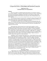
Consider the following example: “A biologist who
studies spiders believes that not only do female green
lynx spiders tend to be longer than their male
counterparts, but also that the lengths of the female
spiders seem to vary more than those of the male spiders.
We shall test whether this latter belief is true.”
Green lynx spider attacking a wasp
Here are data for the lengths of lynx spiders in millimeters:
Lengths of males
5.20 4.70 5.75 7.50 6.45 6.55 4.70 4.80 5.95
5.20 6.35 6.95 5.70 6.20 5.40 6.20 5.85 6.80
5.65 5.50 5.65 5.85 5.75 6.35 5.75 5.95 5.90
7.00 6.10 5.80
Lengths of females
8.25 9.95 5.90 7.05 8.45 7.55 9.80 10.80 6.60
7.55 8.10 9.10 6.10 9.30 8.75 7.00 7.80 8.00
9.00 6.30 8.35 8.70 8.00 7.50 9.50 8.30 7.05
8.30 7.95 9.60
We will assume that these are independent
simple random samples, and that the shapes
of the accompanying histograms are
approximately Normal. Thus, we are
justified in applying the 2-sample F-test for
comparing standard deviations. The
hypotheses are
H 0 : σ M = σ F and H a : σ M < σ F
where M is the male length and F is the
female length variable, respectively.
The F statistic is s F 2 /s M
2
= 3.21 with a
degrees of freedom of (29,29) and a p-value
of 0.0012.
19

Academic Forum 26 2008-09
The small p-value is evidence that the variance in the lengths of the females is greater than that
of the males. However, doing a 2-sample t-test will provide evidence that female lynx spiders
are longer on average than male lynx spiders. Since the female spiders tend to be longer, it
would be more appropriate to compare the sex difference in length for the lynx spider using a
statistic that measures variation relative to length. The coefficient of variation is such a statistic
s
and is defined to be CV = 100 . For the above data,
x
CV M = 100*.663/5.92 = 11.2 and CV F = 100*1.19/8.15 = 14.6, so CV M < CV F ,
but is this difference significant? We will need to determine the distribution of the CV random
s
variable, so for simplicity the 100 in the formula will be dropped and we redefine CV = .
x
We will assume for the remainder of this paper that X
1
, X
2,...,
X
n
is a simple random sample
from N ( µ , σ ) where µ > 0.
Recall the following theorem:
1
Theorem X =
n
n
∑ X j
j=
1
2
( n −1)
S 2
~ χ ( n −1).
2
σ
1 ⎛ σ ⎞
S = ∑ X − X j
are independent, and X ~ N⎜µ,
⎟ and
n −1
j=
1
⎝ n ⎠
n
and ( ) 2
2
We will derive the distribution of the standard deviation. Recall that the probability density
function of ~ 2 2 2
u e
U χ ( n −1)
is fU
( u)
= , u > 0, n = 2,3,...
. Write
n−1
⎛ n −1⎞
2
Γ⎜
⎟2
⎝ 2 ⎠
S =
2
σ ( n −1)
S
⋅
2
( n −1)
σ
2
=
f ( s)
= f
S
σ
n −1
U
1
=
⎛ n −1⎞
Γ⎜
⎟2
⎝ 2 ⎠
n−2
s
=
⎛ n −1⎞
Γ⎜
⎟2
⎝ 2 ⎠
n−1
2
n−3
2
U
du
( u)
ds
n−3
u
−
. Apply the change-of-variable technique to obtain
⎡(
n −1)
s
⎢ 2
⎣ σ
2
⎡(
n −1)
⎤
⎢ 2 ⎥
⎣ σ ⎦
⎤
⎥
⎦
n−1
2
n−3
2
⎡ ( n −1)
s
exp⎢−
2
⎣ 2σ
⎡ ( n −1)
s
exp⎢−
2
⎣ 2σ
2
2
⎤
⎥
⎦
d
ds
⎤
⎥,
s > 0
⎦
⎡(
n −1)
s
⎢ 2
⎣ σ
2
⎤
⎥
⎦
20

Academic Forum 26 2008-09
Here are graphs of some probability distribution functions for the standard deviation and a
formula for its mean and variance:
Graph of S pdf for n=2,3,4,5 using σ=1
E[
S]
=
⎛ n ⎞
2Γ⎜
⎟
⎝ 2 ⎠
−
σ → σ
⎛ n −1⎞
n −1Γ⎜
⎟
⎝ 2 ⎠
2
⎡ ⎛ n ⎞
⎢ 2Γ⎜
⎟
⎢ ⎝ 2
Var[
S]
= 1 −
⎠
⎢
⎛ n −1⎞
⎢ ( n −1)
Γ⎜
⎟
⎢⎣
⎝ 2 ⎠
2
as n → ∞
⎤
⎥
⎥ 2
σ
⎥
⎥
⎥⎦
Mean and Variance of S
→ 0 as n → ∞
To find a formula for the distribution of the CV, consider the joint distribution of ( X , S)
. By
independence, the joint probability density function is
f with support +
R × R . The
probability density function for S was derived earlier, and the probability mass function for is
2
n ⎛ n(
x − µ ) ⎞
easily computed to be f X
( x)
= exp
, ∈ R
2
2
⎜−
2
⎟ x . Therefore, the cumulative
πσ ⎝ σ ⎠
distribution function for CV is
⎡ S ⎤
FCV
( c)
= P⎢
≤ c⎥
= P[ ( S ≤ cX ) ∩ ( X > 0)
] + P[
X < 0]
⎣ X ⎦
(If n is sufficiently large, then
∞ cx
= f ( x)
f ( s)
dsdx + P[
X < 0], c > 0
P [ CV < 0] ≈ 0.)
∫ ∫
0 0
X
S
f X S
Differentiate the
cumulative
distribution
function to obtain
the probability
density function:
=
∞
∫
0
⎛ n ⎞
= ⎜ ⎟
⎝ π ⎠
c > 0
f
CV
n ⎡ n(
x − µ )
exp⎢−
2
2πσ
⎣ 2σ
1
2
c
n−2
( n −1)
⎛ n −1⎞
n
Γ⎜
⎟σ
2
⎝ 2 ⎠
∞
'
( c)
= FCV
( c)
= ∫ f
n−1
2
n−2
2
2
⎤
⎥
⎦
0
( cx)
X
n−2
⎛ n −1⎞
Γ⎜
⎟2
⎝ 2 ⎠
2
⎡ nµ
⎤
exp⎢
−
2 ⎥
⎣ 2σ
⎦
( x)
f
∞
∫
0
x
n−3
2
x
S
n−1
d(
cx)
( cx)
dx + 0
dc
⎡n
−1⎤
⎢ 2
⎣ σ ⎥
⎦
n−1
2
⎡ ( n −1)(
cx)
exp⎢−
2
⎣ 2σ
2
⎡ ( n −1)
c + n
exp⎢−
x
2
⎣ 2σ
2
2
⎤
⎥dx
⎦
nµ
x ⎤
+ ,
2 ⎥dx
σ ⎦
21

Academic Forum 26 2008-09
For the case 2, this formula simplifies to f CV
(c) =
where
erf( z)
=
2
z
∫ − 2
t
e
0
π
system
Derive can find a formula for
small n. Here are graphs of the
CV for n = 2 ,3,4,5; µ = 1; σ = 1.
The areas under these curves are
.921, .958, .977, .987,
respectively. These areas are less
than 1 because µ and n are small
and the P [ CV < 0]
term in the
derivation of the probability
density function was ignored.
However, note that the area under
the probability density function
appears to converge to 1 rapidly
as n converges to infinity.
dt . I could not find general formula for all n, but the computer algebra
Since it appeared hopeless to find a formula for the distribution of the CV for 30, I
attempted to directly compute the probability using
P[
CV
< CV
. However, both Derive and Maple were unable to compute f M or f F because n=30 was
apparently too large. For example,
M
F
] =
∞ c M
∫ ∫
0 0
f
M
( c
M
) f
F
( c
F
) dc dc
F
M
could not be evaluated. My last approach was to try a simulation which was successful.
One thousand samples of size 30 were simulated using the accompanying TI-nspire program.
The parameters µ M =5.92, σ M =0.663, µ F =8.15, σ F =1.18 were estimated from the sample
statistics. Here are the histograms for the simulated coefficients of variation:
22

Academic Forum 26 2008-09
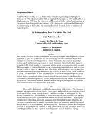
The variable mcv is the male CV, and the
variable fcv is the female CV,
respectively. The accompanying diagram
is a typical Law-of- Large Numbers graph
showing the empirical probability verses
the number of trials generated using the
above program. This probability estimated
using 1000 gives
P [ CV M
< CVF
] ≈ 0.923 . This probability
is less than 0.95, so this provides evidence
that the female spider CV does not appear
to be significantly larger than the male
spider CV.
23

Academic Forum 26 2008-09
Conclusion
Unless the distributions can be modeled with simpler functions, it is impractical to directly do
statistical inference using the CV. Also, perhaps simulations should not be overlooked as an
important tool.
It appears that the mean of CV is approximately σ/µ, and its variance approaches zero as n
approaches infinity. Further investigation would be to provide rigorous proofs or numerical
evidence for these conjectures.
References
• Probability and Statistical Inference by Hogg and Tanis , 7th edition ©2006 Pearson.
• http://creatures.ifas.ufl.edu/beneficial/green_lynx04.htm
Biography
Michael Lloyd received his B.S in Chemical Engineering in 1984 and accepted a position at
Henderson State University in 1993 after earning his Ph.D. in Mathematics from Kansas State
University. He has presented papers at meetings of the Academy of Economics and Finance,
the American Mathematical Society, the Arkansas Conference on Teaching, the Mathematical
Association of America, and the Southwest Arkansas Council of Teachers of Mathematics. He
has also been an AP statistics consultant since 2001 and a member of the American Statistical
Association.
24