PDF 4:1

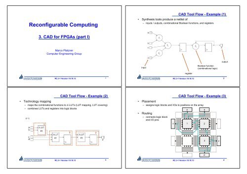
Reconfigurable Computing 

CAD Tool Flow - Example (1) 

• Synthesis tools produce a netlist of 

– inputs / outputs, combinational Boolean functions, and registers 

3. CAD for FPGAs (part I) 

Marco Platzner 

Computer Engineering Group 

output 

input 

Boolean function 

(combinational logic) 

register 

RC.3-1 Version 10.10.13 1 

RC.3-1 Version 10.10.13 2 


• Technology mapping 

– maps the combinational functions to K-LUTs (LUT mapping, LUT covering) 

– combines LUTs and registers into logic blocks 

K=3: 

1 


• Placement 

– assigns logic blocks and I/Os to positions on the array 

• Routing 

– connects logic block 

and I/O pins 

c 

a 

b 

1 2 

2 3 

3 

z 

d 

RC.3-1 Version 10.10.13 3 

RC.3-1 Version 10.10.13 4

design entry 

optimization 

& synthesis 

technology 

mapping 

placement 

CAD for FPGAs - Contents 

– Technology mapping 

! network decomposition 

! LUT mapping 

! sequential mapping 

! logic block packing (VPack) 

– Placement 

! simulated annealing (VPR) 

Optimization Problems 

• Objectives 

– area: minimize the required chip area 

– delay: minimize the delay on the critical path 

– power: minimize the dynamic power dissipation 

– routability: facilitate successful routing 

! these goals are often conflicting, eg. area and delay 

routing 

simulation 

generation 

of bitfile 

– Routing 

! Pathfinder (VPR) 

– Timing analysis & delay modeling 

• Cost models (estimates) 

– area models: number of LUTs (logic blocks), routing area 

– delay models: logic block delay, routing delay 

– power models: the power can be estimated by the output load 

capacitances and transition frequencies 

RC.3-1 Version 10.10.13 5 

RC.3-1 Version 10.10.13 6 

optimization 

& synthesis 

technology 

mapping 

node decomposition 

LUT mapping 

Technology Mapping 

sometimes called 

FPGA logic synthesis 

Boolean Network – Definitions (1) 

• A Boolean network is a directed acyclic graph (DAG) G=(V,E), where 

the nodes v !V represent logic functions, primary inputs (PIs), or 

primary outputs (POs). A directed edge (v,w) ! E denotes that the 

output of v is an input of w. 

1 2 3 4 5 6 7 8 

placement 

logic block packing 

p q t 

o 

routing 

s 

w 

x 

– node decomposition 

! split combinational functions into nodes with at most K inputs 

! is done during synthesis or during technology mapping 

r u y 

v 

z 

9 10 11 

RC.3-1 Version 10.10.13 7 

RC.3-1 Version 10.10.13 8


• Given a directed edge (v,w) ! E, v is a fanin of w, and w is a fanout of v. 

A PI has no fanin; a PO has no fanout. If there is a path from a node r 

to a node s, r is a predecessor of s, and s is a successor of r. 

• The level of a node v is the maximum number of edges on any path 

from a PI to v. The depth of a network is the largest level of any node. 

• The set of fanins of node v is called input(v). A node is K-feasible, if 

|input(v)| ! K. If every node in a network is K-feasible, the network is 

K-bounded. 


• The set of fanouts of a node v is called output(v). A node v is fanoutfree, 

if |output(v)| ! 1. 

• The network is called a 

– tree if every node (including PIs) is fanout-free and there is only one PO 

– leaf-DAG if every non-PI node is fanout-free 

– general network otherwise 

RC.3-1 Version 10.10.13 9 

RC.3-1 Version 10.10.13 10 


• A cone of node v is denoted as C v and consists of v and some non-PI 

predecessors such that for any node w in C v there exists a path from w 

to v that is entirely in C v . The node v is the root of C v . The maximum 

cone of v is denoted as MC v and consists of all non-PI predecessors 

of v. 

N v 

Boolean Network - Example 

1 2 3 4 5 6 7 8 

p q t o 

• The fanin network of v is denoted as N v and extends MC v by including 

all PI predecessors of v. 

MC v 

s 

w 

x 

• A fanout-free cone (FFC) is a cone in which the fanouts of every node 

(except the root node) are in the cone. For each node v, there exists a 

unique maximum fanout-free cone MFFC v . 

• For each node v, there exists also a maximum tree MT v of non-PI nodes. 

MT " MFFC " MC ! N 

v 

v 

v 

v 

MFFC v 

MT v 

r u y 

v 

z 

9 10 11 

RC.3-1 Version 10.10.13 11 

RC.3-1 Version 10.10.13 12

Network Decomposition 

• Some nodes in the network might not be K-feasible 

! decompose such nodes into smaller ones that are K-feasible 

– a decomposed (ie. a K-bounded) network is already a trivial LUT mapping 

• Classification of decomposition methods 

– structural decomposition methods 

! for node functions that are basic gates 

! some methods: balanced tree decomposition, minimum tree decomposition, 

Huffman tree decomposition, bin-packing decomposition 

– symbolic decomposition methods 

! for more complex node functions 

! some methods: AND/OR decomposition, algebraic division based extraction, 

OBDD based extraction 

– Boolean decomposition methods 

! for more complex node functions 

! some methods: cofactoring, function-based decomposition 

RC.3-1 Version 10.10.13 13 

Structural Decomposition 

• For simple node functions (AND, OR, XOR, !.) 

– associative and commutative properties allow arbitrary groupings 

of the inputs 

a + (b + c) = (a + b) + c a + b = b + a 

– structural decomposition is used in classical logic synthesis systems 

that target simple gates (eg. 2-NAND) 

– early FPGA logic synthesis systems used the same approach 

1. decompose the network into simple gates 

2. map the simple gate network to LUTs 

• Problem statement: Decompose a simple gate node v, 

input(v) = {w 1 , …w m }, (m > K), into a 

tree of nodes of input size K or less. 

RC.3-1 Version 10.10.13 14 

Balanced Tree Decomposition 

• Algorithm 

1. divide input(v) into K groups of (nearly) equal size (balancing constraint) 

2. introduce K new gates, each combining the inputs from one group; 

these K new gates form the input of the root gate v that replaces v 

3. apply recursively for all nodes with input size larger than K 

• Properties 

– gives minimum-depth decomposition of v 

– the size (number of gates) might not be minimum (for K>2) 

Minimum Tree Decomposition 

• Replaces the balancing constraint by a FIFO (first-in, first-out) list 

• Algorithm 

1. construct a list L of nodes in input(v) in FIFO order 

2. iterate: a. remove the first K nodes from L and create a new node with these 

nodes as inputs 

b. put the new node back to L in FIFO order 

c. stop when |L| ! K; |L| is the number of entries in the FIFO 

9-OR, K=2 

5 4 

3 

RC.3-1 Version 10.10.13 15 


– gives minimum-depth and minimum-size decomposition of v 

$ m % 1" 

(for |input(v)| = m, the minimum number of gates is D = ) 

# K % 1! 

– runtime complexity O(m) 

RC.3-1 Version 10.10.13 16

Huffman Tree Decomposition 

• Balanced tree decomposition 

– does not give the minimum number of levels for the overall network when 

the inputs of v have different levels 

! the Huffman tree decomposition uses a different sorting rule for the list L 

• Algorithm 

1. construct a list L of nodes in input(v) sorted according to non-decreasing 

levels 

2. iterate a. remove the first K nodes from L and create a new node with these 

nodes as inputs 

b. put the new node back to L (the list must remain sorted) 

c. stop when |L| ! K 


– when done for all not K-feasible nodes of the network in topological order 

(from the PIs to the POs), the decomposed network is delay-optimal 

– runtime complexity O(m.log(m)) 

RC.3-1 Version 10.10.13 17 

Symbolic Decomposition 

• For more complex node functions 

– the node function is specified in some symbolic representation, eg. as 

Boolean expression, sum-of-products (SOP), ordered binary decision 

diagram (OBDD), ! 

– symbolic decomposition techniques try to extract K-feasible subfunctions 

from these representations 

• Some methods 

– AND/OR decomposition 

! when the node function is given as SOP, split it into a disjunction of conjunctions 

! if the resulting subfunctions are not K-feasible, apply structural decomposition 

– algebraic division based extraction 

! when the node function is given as Boolean expression, view it as an algebraic 

expression and apply transformations of polynomial algebra (instead of Boolean 

algebra) 

! although weaker, the polynomial algebra allows to perform polynomial division to 

extract kernels and co-kernels as subfunctions 

RC.3-1 Version 10.10.13 18 

Boolean Decomposition 

• For more complex node functions 

– symbolic decomposition works on the symbolic representation of the node 

function, but the specific representation might not be the best one 

– Boolean decomposition works on the Boolean function itself, which is 

independent of the representation 

• Some methods 

– co-factoring 

! uses Shannon expansion to extract cofactors; a cofactor has one fewer variable 

! limited to cofactors as subfunctions f x! 

f + x f 

a b c d 

z 

f z 

= abc( de + de) 

= d( 

abce) 

+ d( 

abce) 

e 

= 

x= 1 

! 

x=0 

a b 

z 

c e 

z 

a b 

z 

c e 

RC.3-1 Version 10.10.13 19 

d 

• Some methods (contd) 

– functional decomposition 

! exploits arbitrary subfunctions 

i, 

j, 

m # r 

Boolean Decomposition 

( y ( x … x ),… 

y ( x … x ), x ,… 

x ) 

f ( x1, 

… xr 

) = g 

1 1 i m 1 

i " j ! 1 > 0 

! the first j-1 variables of the function are encoded by m new variables 

! y 1 …y m are the econding functions, g is the base function 

! if i=j-1 the decomposition is disjunctive, x 1 …x i is the bound set and x j …x r the free 

set 

! there are several methods for partitioning the variables into bound and free sets 

and finding encoding and base functions, eg. Ashenhurst decomposition, Roth- 

Karp decomposition, ! 

– functional decomposition techniques are very important for LUT-based logic 

synthesis, because LUTs can implement any function that is K-feasible (the 

specific structure or symbolic representation is irrelevant) 

RC.3-1 Version 10.10.13 20 

i 

j 

r

optimization 

& synthesis 

technology 

mapping 

placement 

routing 


LUT mapping 





• Given is 

– a K-bounded tree T r with root node r 

Tree Mapping (1) 

– a mapping where LUT r implements r, which means that there is also a 

mapping for each subtree T w rooted at w ! input(LUT r ) 

– the number of LUTs in is given by 

! 

area 

M Tw 

M Tr 

M Tr 

( M 

T 

) = 1+ 

! area( M ) 

r 

T w 

w" 

input ( LUTr 

) 

area( M Tr 

) 

– LUT mapping 

! maps K-bounded Boolean networks into K-LUTs 

r 

K=3 

RC.3-1 Version 10.10.13 21 

RC.3-1 Version 10.10.13 22 

• The area optimal mapping 

area 

% 

& = + ' 

LUTr 

$ w input ( 

* 

* 

( M ) min 1 area( M ) 

Tr 

( LUTr 

) 

Tw 

# 

" 

! 


* 

M Tr 

– can be computed from the area-optimal mappings of the subtrees 


• How can the best LUT r be found? 

– by enumerating all K-feasible cones rooted at r (all possible LUT r ) 

– by a greedy method TreeMap that has been shown to be optimal 

! with input(v) = {w 1 , …w m }, and 

the following ordering of LUT indices 

{ } 

input LUTw ) !!! 

input( 

LUT w 

) 

( 

1 m 

! set LUT 

where s is the largest index such that LUT 

v 

= v " LUTw 

v 

i 

remains K-feasible 

i! 

s 

r 

two possible LUT r 

K=3 

• Algorithm TreeMap 

– go through the tree in topological order 

1. at each node v, sort the input LUTs in increasing order of input size 

2. greedily expand the cone C v to cover as many input LUTs as possible in that order 

3. set LUT v =C v 


– gives the area-optimal mapping for trees 

– runtime complexity O(max{K,log(n)·n}); n is the number of nodes in the tree 

RC.3-1 Version 10.10.13 23 

RC.3-1 Version 10.10.13 24


• Remarks 

– to find a delay-optimal mapping with TreeMap, sort the LUTs by decreasing 

order of depths 

– TreeMap is optimal only for trees, general networks must be partitioned into 

a set of MT (maximum trees) which are mapped independently 

! which does not give an optimal mapping for the overall circuit 

MFFC Mapping 

• In MFFCs, internal nodes may have multiple fanouts 

– LUTs may overlap, ie. a node may be implemented in several LUTs 

– a mapping without such overlaps is called a duplication-free mapping 

– a mapping with such overlaps is called mapping with logic duplication and 

can lead to less delay and less area (!) 

– MMFC mapping with logic duplication is as difficult as general network 

mapping 

– for leaf-DAGs there exists also a delay-optimal version of TreeMap, 

but no area-optimal version 

K=4 

r 

RC.3-1 Version 10.10.13 25 

RC.3-1 Version 10.10.13 26 

General Network Mapping (1) 

• General networks 

– can be split into MTs or MFFCs that are mapped independently 

– however, direct mapping of general networks can produce better results 

• Delay minimization 

– we only have to look at the levels of the nodes, the number of LUTs is not 

important (ie. we can use logic duplication) 

! the delay-optimal mapping of a node v depends only on the mapping of 

nodes in N v ; the delay of node v is 1 plus the delay of N v -LUT v 

– we go through the network in topological order and, at each node v, select 

the LUT v that minimizes the delay of N v -LUT v 

! there are several algorithms to find the delay-optimal LUT v (eg. dag-map) 


• Algorithm dag-map 

– assign each PI node v of the network a label l(v)=0 

– go through the network in topological order, for each node v 

! let p be the largest label of the nodes in input(v) 

! l(v)=p if the set of nodes w ! N v with label l(w)=p form a K-feasible cone C v ; 

otherwise, l(v)=p+1 

! LUT v = {w | w ! N v , l(w)=l(v)} (plus duplicated logic, if required) 


– runtime complexity O(n 2 ) for a network with n nodes 

– delay-optimal only if the network is monotonic under LUT mapping 

! if a cone C w is not K-feasible, then any larger cone C v containing C w cannot 

be K-feasible 

! general networks are not always monotonic, they can have reconvergent 

fanout paths 

RC.3-1 Version 10.10.13 27 

RC.3-1 Version 10.10.13 28


• Delay minimization 

– there is also a delay-optimal algorithm for non-monotonic general 

networks: flowmap 

– flowmap has a runtime complexity of O(Kmn), with m as the number of 

edges and n as the number of nodes of the general network 

• Area minimization for general networks 

– is a more difficult problem than delay minimization because we have to 

consider overlapping sub-networks 

– there exist several algorithms 

! exact algorithms based on enumeration and Integer Linear Programs (ILP) 

! heuristic algorithms that use rules to select the nodes that will be covered 

by a LUT 

RC.3-1 Version 10.10.13 29 

Overview - Decomposition & LUT Mappers 

– Chortle family 

! Chortle [1990] partitions simple-gate networks into trees, node 

decomposition, area-optimal mapping by enumeration 

! Chortle-crf [1991] decomposition and mapping by FFD bin-packing, 

further heuristic improvements for leaf-DAGs 

! Chortle-d [1991] delay minimization for leaf-DAGs 

– MIS family 

! MIS-pga [1990], symbolic and Boolean decomposition, 

MIS-pga (new) [1991] area-minimization for general networks 

! MIS-pga (delay) [1991] delay minimization for general networks 

– TechMap family 

! TechMap [1992], TechMap-L [1992], TechMap-D [1993] for simple-gate 

networks 

– FlowMap family 

! DAG-Map [1992], FlowMap [1992] delay-optimal mapping for general networks 

! FlowMap-r [1993], FlowSYN [1993], diverse improvements 

FlowMap-d [1993], CutMap [1995] 

RC.3-1 Version 10.10.13 30 

Sequential Mapping 

Retiming - Example 

• Technology mapping algorithms usually 

1. split a sequential circuit into several combinational circuits 

2. map the combinational circuits to LUTs independently 

3. assemble LUTs and registers to the final technology-mapped netlist 

a 

b 

d 

e 

retiming 

a 

b 

d 

e 

c 

c 

• Direct sequential mapping techniques 

– do not split the sequential circuit into independent combinational 

circuits, but work on the overall netlist 

– common treatment of combinational functions and registers allows for 

! more combinational optimizations (area and delay) 

! register optimization (minimize number of registers) 

– most important transformation: retiming, ie. shifting registers to different 

positions in the netlist without changing the function of the circuit 

combinational 

LUT mapping 

K=4 

a 

b 

d 

e 

a 

b 

c 

combinational 

LUT mapping 

K=4 

d 

e 

example: 

c 

register 

optimization 

4-LUT 

RC.3-1 Version 10.10.13 31 

RC.3-1 Version 10.10.13 32


Logic Block Packing (1) 

optimization 

& synthesis 

technology 

mapping 


LUT mapping 



• Combines LUTs and registers into logic blocks 

– simple logic block (basic logic element, BLE) consists of a single LUT 

and a register 

– cluster-based logic block consists of several BLEs 

placement 


• Basic logic element (BLE) 

– characterized by K 

routing 

– logic block packing 

! combines LUTs and registers into logic blocks and/or clusters of logic blocks 

RC.3-1 Version 10.10.13 33 

RC.3-1 Version 10.10.13 34 

• A cluster is characterized by 

– the BLE parameter K 

– the number of BLEs in the cluster N 

– the number of cluster inputs I, I < K.N 

Cluster-based Logic Blocks (1) 

• Example: K = 3, N = 3, I = 6 

! 9 multiplexors 9:1 

Cluster-based Logic Blocks (2) 

• Fully-connected clusters 

– any cluster input or cluster output can 

connect to any BLE input 

– the connections are realized with 

multiplexors 

– full connectivity is expensive but 

simplifies the packing problem 

– some commercial FPGAs are fully 

connected (eg. Altera 8K/10K), 

others are nearly fully connected 

(eg. Xilinx XC5200) 

RC.3-1 Version 10.10.13 35 

• Packing goals 

– pack connected BLEs (LUTs) into one cluster to minimize the number of 

signals to be routed between clusters 

– pack the clusters as full as possible to minimize the number of required 

clusters 

RC.3-1 Version 10.10.13 36

• Logic block packing is a clustering problem 

– for logic block packing, greedy heuristics are used 

(eg. algorithms VPack, T-VPack) 

Logic Block Packing (2) 

Algorithm VPack (1) 

• VPack – step 1 

– pack LUTs and registers to BLEs by following pattern matching rule 

• Algorithm VPack 

– input: netlist of LUTs and registers 

– output: netlist of clusters 

– parameters: N, I, K 

– runs in two steps: 

1. pack LUTs with registers into BLEs 

2. pack BLEs into clusters 

LUT followed by a register: 

pack into one BLE 

LUT with fanout followed by a register: 

pack LUT and register into two different BLEs 

RC.3-1 Version 10.10.13 37 

RC.3-1 Version 10.10.13 38 



• VPack – step 2 

– pack BLEs to clusters; runs in two phases 

phase I: 

1. start a new cluster with a seed BLE; the seed BLE is the BLE 

with the most inputs used 

2. greedily pack further BLEs to the cluster using the metric 

attraction(C, BLE) 

3. if the cluster is full, goto 1 and start a new cluster; if the cluster 

is not full, start phase II 

phase II: greedily pack further BLEs to the cluster using the metric 

" cluster inputs (C, BLE) 

UnClusteredBLEs = PatternMatchingToBLEs(netlist); 

Clusters = { }; 

while (UnClusteredBLEs != { }) { 

C = GetBLEWithMostUsedInputs(UnClusteredBLEs); 

while (|C| < N) { 

BestBLE = MaxAttractionLegalBLE(C, UnClusteredBLEs); 

if (BestBLE) == { } ) break; 

} 

UnClusteredBLEs = UnClusteredBLEs \ BestBLE; 

C = C U BestBLE; 

} 

if (|C| < N) { 

while (|C| < N) { 

BestBLE = MinClusterInputIncreaseBLE(C, UnClusteredBLEs); 

} 

UnClusteredBLEs = UnClusteredBLEs \ BestBLE; 

C = C U BestBLE; 

} 

if (!ClusterIsLegaI(C)) 

RestoreToLastLegalState(C, UnClusteredBLEs); 

Clusters = Clusters U C 

phase I 

phase II 

RC.3-1 Version 10.10.13 39 

RC.3-1 Version 10.10.13 40


• MaxAttractionLegalBLE(C, UnClusteredBLEs) 

– attraction(C, BLE) = | nets(BLE) " nets(C) | 

nets(BLE) is the set of inputs and outputs of the BLE 

nets(C) is the set of inputs and outputs of the BLEs in cluster C 

– this metric tends to pack connected BLEs into one cluster 

– a BLE is not added to a cluster if the cluster size would be exceeded 

(ie. if the number of required inputs becomes larger than I) 

• MinClusterInputIncreaseBLE(C, UnClusteredBLEs) 

– " cluster inputs (C, BLE) = | fanin(BLE) | - | nets(BLE) " nets(C) | 

– the number of cluster inputs is allowed to exceeded I, because subsequent 

steps could reduce the number of required inputs 

– if the cluster is illegal at the end, the last legal state of phase II is restored 

Timing-driven VPack (1) 

• Algorithm T-VPack 

– VPack tries to pack clusters full; T-VPack additionally tries to minimize the 

number of intercluster-connections on the critical path 

– the seed and attraction functions of T-VPack depend on the criticality of 

BLEs 

– T-VPack performs timing analysis with three types of delays 

! LogicDelay: delay through a BLE 

! IntraClusterDelay: delay between BLEs in a cluster 

! InterClusterDelay: delay between different clusters, approximated 

by a constant 

• Runtime complexity is O(k max Kn) 

– k max is the maximum number of terminals on any net 

– n is the number of LUTs and registers (BLEs) in the netlist 

RC.3-1 Version 10.10.13 41 

RC.3-1 Version 10.10.13 42 

• Algorithm T-VPack (cont'd) 


• Algorithm T-VPack (contd) 


– the criticality of a connection i is: 

slack( 

i) 

Connection Criticality ( i) 

= 1! 

MaxSlack 

! MaxSlack is the maximum slack of any connection in the circuit 

– seed BLE: the BLE with the highest connection criticality for any of its 

connections 

– attraction function: 

nets( 

BLE) 

! nets( 

C) 

attraction ( C, 

BLE) 

= !" 

Criticalit y ( C, 

BLE) 

+ (1 # !)" 

MaxNets 

! ! is a weighting parameter (" = 0 corresponds to VPack; " = 1 minimizes 

the circuit delay) 

! MaxNets is the maximum nuber of nets that can connect to a BLE (normalization) 

– attracting a BLE to a cluster C: the criticality of the BLE, Criticality(C, BLE), 

is defined as the maximum connection criticality of any connection joining 

BLE to C; if there is no such connection, the criticality is zero 

• Runtime complexity 

– depends on how often timing analysis is done 

! recompute the delays after each packed BLE: O(n 2 ), where n is the no. of BLEs 

! recompute the delays after p packed BLEs: O(n 2 /p) 

! compute the delays only once at the beginning: O(k max Kn), the same as for VPack 

RC.3-1 Version 10.10.13 43 

RC.3-1 Version 10.10.13 44

Selected Literature (1) 

• Digital Design 

– John P. Hayes. Introduction to Digital Logic Design. 

Addison-Wesley, 1993 

– John F. Wakerly. Digital Design: Principles and Practices. 

Addison-Wesley, 4th. Edition, 2006 

– Randy H. Katz, Gaetano Borriello. Contemporary Logic Design. 

Addison-Wesley, 2. Edition, 2005 

– M. Morris Mano, Charles R. Kime, Logic and Computer Design 

Fundamentals. 4th. Edition, Prentice Hall, 2007 

• CAD General 

– G. De Micheli. Synthesis and Optimization of Digital Circuits. 

McGraw-Hill, 1994. 

Selected Literature (2) 

• CAD for FPGAs 

– V. Betz, J. Rose and A. Marquardt. Architecture and CAD for Deep- 

Submicron FPGAs. Kluwer Academic Publishers, 1999. 

– J. Cong and Y. Ding. Combinational Logic Synthesis for LUT Based 

Field Programmable Gate Arrays. ACM Transactions on Design 

Automation of Electronic Systems, 1(2):145–204, April 1996. 

• FPGA Architectures 

– S. Brown and J. Rose. FPGA and CPLD Architectures: A Tutorial. 

IEEE Design & Test of Computers, pages 42–57, Summer 1996. 

– S. Brown, R.J. Francis, J. Rose, and Z.G. Vranesic. Field- 

Programmable Gate Arrays. Kluwer Academic Publishers, 1992. 

– J. Rose, A. El Gamal, and A. Sangiovanni-Vincentelli. Architecture of 

Field-Programmable Gate Arrays. Proceedings of the IEEE, 81(7): 

1013–1029, July 1993. 

RC.3-1 Version 10.10.13 45 

RC.3-1 Version 10.10.13 46

PDF 4:1

You also want an ePaper? Increase the reach of your titles

Delete template?

Save as template?