Equivariant Embeddings of Algebraic Groups

c○ Copyright by David Charles Murphy, 2004

EQUIVARIANT EMBEDDINGS OF ALGEBRAIC GROUPS 

BY 

DAVID CHARLES MURPHY 

B.A., Western Michigan University, 1996 

M.S., University of Illinois at Urbana-Champaign, 1998 

DISSERTATION 

Submitted in partial fulfillment of the requirements 

for the degree of Doctor of Philosophy in Mathematics 

in the Graduate College of the 

University of Illinois at Urbana-Champaign, 2004 

Urbana, Illinois

Abstract 

We classify embeddings of algebraic groups as open orbits in affine varieties, generalizing results 

from toric geometry to connected reductive groups. In particular, we show that an embedding is 

determined by the set of one-parameter subgroups that have a limit in the embedding. We then 

investigate the structure of such sets of one-parameter subgroups and how their properties reflect 

properties of the associated embedding. 

iii

To my parents in gratitude for all of their support and encouragement 

iv

Acknowledgements 

This thesis would not have been possible without the help, patience, and wisdom of my advisers, 

Robert M. Fossum and William J. Haboush. Specifically, I would like to thank Professor Haboush 

for his great help in developing my understanding of the algebraic geometry and representation 

theory used in this dissertation and Professor Fossum for his algebraic insights. 

I also wish to 

thank the other members of my committee, Professors Maarten Bergvelt, Phillip Griffith and Rinat 

Kedem. 

I would like to thank Professor Griffith, in his capacity as the Director of Graduate Studies. He 

and his staff, Lori Dick and Marci Blocher, have constantly helped and encouraged me during my 

years as a graduate student. 

Finally, I am very grateful to my fellow graduate student and friend, Joshua Mullet, for the 

many conversations we have had about our work and the new ideas these discussions generated. 

v

Table of Contents 

Chapter 1 Introduction . . . . . . . . . . . . . . . . . . . . . . . . . . . . . . . . . . . . . . . 1 

1.1 Toric varieties . . . . . . . . . . . . . . . . . . . . . . . . . . . . . . . . . . . . . . . . 2 

1.2 Luna–Vust theory and spherical varieties . . . . . . . . . . . . . . . . . . . . . . . . . 3 

1.3 The “wonderful compactification” . . . . . . . . . . . . . . . . . . . . . . . . . . . . . 6 

1.4 Affine group embeddings . . . . . . . . . . . . . . . . . . . . . . . . . . . . . . . . . . 7 

Chapter 2 Toric varieties and group embeddings . . . . . . . . . . . . . . . . . . . . . . . . 11 

2.1 Toric varieties as group embeddings . . . . . . . . . . . . . . . . . . . . . . . . . . . 12 

2.1.1 Affine toric varieties and one-parameter subgroups . . . . . . . . . . . . . . . 12 

2.1.2 Toric varieties from fans . . . . . . . . . . . . . . . . . . . . . . . . . . . . . . 14 

2.1.3 The torus action . . . . . . . . . . . . . . . . . . . . . . . . . . . . . . . . . . 15 

2.1.4 Equivariant divisors in toric varieties . . . . . . . . . . . . . . . . . . . . . . . 16 

2.2 Toric varieties in group embeddings . . . . . . . . . . . . . . . . . . . . . . . . . . . . 17 

2.2.1 Regular compactifications . . . . . . . . . . . . . . . . . . . . . . . . . . . . . 17 

2.2.2 A family of left-equivariant SL n -embeddings . . . . . . . . . . . . . . . . . . 19 

2.3 Group embeddings from toric varieties . . . . . . . . . . . . . . . . . . . . . . . . . . 22 

2.3.1 Mumford’s group embeddings . . . . . . . . . . . . . . . . . . . . . . . . . . . 22 

2.3.2 Group embeddings constructed using flag varieties . . . . . . . . . . . . . . . 23 

Chapter 3 Affine group embeddings . . . . . . . . . . . . . . . . . . . . . . . . . . . . . . . . 34 

3.1 Group actions on affine varieties . . . . . . . . . . . . . . . . . . . . . . . . . . . . . 34 

3.2 Classification of affine group embeddings . . . . . . . . . . . . . . . . . . . . . . . . . 39 

3.2.1 Limits of one-parameter subgroups . . . . . . . . . . . . . . . . . . . . . . . . 39 

3.2.2 States and strongly convex lattice cones . . . . . . . . . . . . . . . . . . . . . 48 

3.2.3 Classification theorem . . . . . . . . . . . . . . . . . . . . . . . . . . . . . . . 54 

3.3 Functoriality of our classification . . . . . . . . . . . . . . . . . . . . . . . . . . . . . 58 

3.3.1 Equivariant morphisms between affine G-embeddings . . . . . . . . . . . . . . 58 

3.3.2 Biequivariant resolutions . . . . . . . . . . . . . . . . . . . . . . . . . . . . . . 60 

References . . . . . . . . . . . . . . . . . . . . . . . . . . . . . . . . . . . . . . . . . . . . . . . 67 

Vita . . . . . . . . . . . . . . . . . . . . . . . . . . . . . . . . . . . . . . . . . . . . . . . . . . 71 

vi

Chapter 1 

Introduction 

A basic problem in algebraic geometry is the study of algebraic actions. Even actions with a dense 

orbit are not well understood. A quasihomogeneous variety is a normal G-variety X possessing an 

open orbit isomorphic to G/H, for some closed subgroup H of G. Toric varieties are an important 

family of quasihomogeneous varieties, where G is an algebraic torus and H is its trivial subgroup. 

A partial classification of quasihomogeneous varieties was obtained in the important paper of Luna 

and Vust [30], written twenty years ago. 

Their classification seeks to generalize that of toric 

varieties, but it is only feasible in special cases. 

The goal of this dissertation is to solve the 

equivariant classification problem for one case not covered in [30], namely the classification of 

quasihomogeneous varieties in which H is trivial. 

In this introduction, we review the history of and some of the results that are essential to our 

problem. As mentioned above, toric varieties are the natural place to begin, so we discuss them 

in the first section. After that, we present a short overview of Luna and Vust’s paper [30] and 

some of the work that has been done in an attempt to exploit the Luna–Vust classification in cases 

that initially appear to be outside the scope of their original work. This chapter concludes with an 

overview of our results. 

First, we establish a few conventions that will be used throughout this thesis and notation 

that we use freely hereafter. We will always work over a ground field k, which we assume to be 

algebraically closed and of characteristic zero. The term variety will refer to a separated, integral 

scheme of finite type over k. All algebraic groups are assumed to be linear and defined over k, and 

will be denoted by letters such as G and H. In particular, G will refer to a connected reductive 

linear algebraic group defined over k, unless otherwise stipulated. 

1

1.1 Toric varieties 

The theory of toric varieties is a well-established and valuable class of examples for the study 

of equivariant algebraic geometry. Toric varieties were introduced by Demazure [13] in the early 

1970s, in which he classified all smooth toric varieties. The classification of all toric varieties was 

accomplished three years later by Kempf–Knudsen–Mumford–Saint-Donat [28] using fans in the 

vector space associated to the set of one-parameter subgroups of a torus. 

We begin by recalling the definition of toric varieties. Suppose T is an algebraic torus. Since 

we are assuming that our ground field k is algebraically closed, T ∼ = G r m for some r, where G m = 

Spec k[x, x −1 ] is the multiplicative group scheme of k. 

Definition 1. A toric variety is a normal variety X containing an algebraic torus T as an open 

subset such that the translations of T on itself extend to give an action of T on X. 

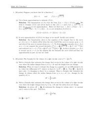
Example 1 (A toric variety and its fan). Consider T = G 2 m. Then X = P 2 is a toric variety for 

T as it is normal, contains T as the open subvariety {[t 0 : t 1 : t 2 ] : t 0 , t 1 , t 2 ≠ 0}, and has T -action 

given by [t 0 : t 1 : t 2 ] · [x 0 : x 1 : x 2 ] = [t 0 x 0 : t 1 x 1 : t 2 x 2 ]. There are seven open affine T -subvarieties 

of X, which are glued together along common open affine subvarieties within X. This is recorded 

by the “fan” below, consisting of seven cones: 3 are two dimensional (cones 1 , 2 , 3 ), 3 are one 

dimensional (cones 4 , 5 , 6 ) and one is zero dimensional (cone 7 ). 

• • 5 • 1 

2 • • • • 

• • 7 • 4 

• • • • • 

 

6 • • 3 • 

The two dimensional cones each correspond to T -stable affine spaces in X, U i = {[x 0 : x 1 : x 2 ] : 

2

x i ≠ 0} for i = 0, 1, 2, the one dimensional cones correspond to the T -stable affine subvarieties 

U ij = {[x 0 : x 1 : x 2 ] : x i , x j ≠ 0}, and the zero dimensional cone corresponds to T itself, viewed as 

the subvariety {[t 0 : t 1 : t 2 ] : t 0 , t 1 , t 2 ≠ 0}. 

Toric varieties play an important role both in algebraic and combinatorial geometry due to the 

nature of their classification. In particular, toric varieties are useful for the calculation of the number 

of lattice points in polytopes in combinatorial geometry. Their applications in algebraic geometry 

are numerous as well, especially as a “source of interesting, yet manageable examples” [17]. Toric 

varieties also play a critical role in mirror symmetry [11]. 

Due to the relationship between algebraic geometry and combinatorial geometry afforded by 

the classification of toric varieties, many have recently preferred to introduce and even define toric 

varieties not in terms of the torus within, but instead in terms of their combinatorial classification. 

However, this separation from the roots of the subject has had negative consequences. By studying 

toric varieties as varieties whose transition functions are monomials or via Cox’s homogeneous coordinate 

ring [10], as many now do, the role toric varieties play as part of the equivariant classification 

program has been diminished. 

In the introduction to [12], after motivating the importance of toric varieties and their relationship 

with combinatorial geometry, Danilov returns to their original definition and proposes “An 

extension of this theory would seem possible, in which the torus T is replaced by an arbitrary 

reductive group G” ([12], page 101). 

1.2 Luna–Vust theory and spherical varieties 

In [30], Luna and Vust began a program to describe up to G-isomorphism varieties admitting an 

action of an algebraic group G. A birational classification of G-varieties (i.e., classifying how G acts 

on fields) may be obtained using Galois cohomology [38]. The second part of the problem requires 

one to describe all G-models of a given function field K with G acting birationally on K. 

Let K be a field of finite type over k. A model of K is a variety X with k(X) = K. We remark 

that all models of K may be glued together to form a large (non-Noetherian, non-separated) scheme 

X = X(K/k). The group G acts on X in a natural way, but this is not an action in the category of 

3

schemes. However, there is a largest open subset X G ⊆ X such that G acts on X G as an algebraic 

group. 

In the paper [30], G is assumed to be reductive and of simply connected type (that is, G is the 

direct product of a torus and a simply connected semisimple group). Furthermore, all G-models 

are assumed to be normal. 

The following theorem of Sumihiro is the basic tool for the local study of G-varieties. 

Theorem 1 ([42], Lemma 8). Let G be a connected linear algebraic group and let X be a normal 

G-variety. Then any point x ∈ X has a G-stable neighborhood X 0 ⊆ X admitting an equivariant 

locally closed embedding in a projective space. 

Therefore, every regular action of a connected linear algebraic group on a normal variety is 

obtained by patching finitely many linear actions on normal quasi-projective varieties. Thus, if we 

are interested in local properties of a G-model X in a neighborhood of a point x or a subvariety Y , 

we may assume that X is quasi-projective. 

Let X be a quasihomogeneous G-variety with open orbit G/H and k(X) = k(G/H) = K. Let 

B be a Borel subgroup of G. We introduce the following terminology. 

The complexity of the variety X or of the field K, denoted c(X) or c(K) respectively, is the 

transcendence degree of K B . 

Hence c(X) is equal to the codimension of a B-orbit in general 

position on X. 

The set of G-stable discrete Q-valued valuations of K/k that are geometric (that is, correspond 

to prime divisors on a suitable model of K) is denoted V = V(K). Elements of V are called G- 

valuations. Let D = D(G/H) be the set of irreducible subvarieties of G/H of codimension one that 

are not G-stable. The valuation corresponding to a divisor D ∈ D is denoted by v D . Prime divisors 

that are B-stable but not G-stable are called B-divisors. The set of B-divisors is denoted D B . 

Suppose X is a G-model of K, so k(X) = K. Then the complexity measures the codimension 

of a B-orbit in general position on X. When the complexity is ≤ 1, D B is particularly simple. If 

c(X) = 0, G has an open orbit in X, say G/H. In this case, D B is the finite set of the irreducible 

components of the complement of the open orbit of B in G/H. Suppose c(X) = 1. Let G/H be a 

sufficiently generic orbit and let U be the open subset of G/H formed of B-orbits of codimension 

1. Then D ∈ D B implies either D is the closure of a B-orbit in U or D is a component of the 

4

complement of U in G/H. 

Remark 1 ([30], page 220). The Luna–Vust classification strategy is only feasible when c(K) ≤ 1. 

Let P be the set of f ∈ k(G) which are simultaneously eigenvectors of B (acting by left 

translations) and of H (acting by right translations). 

f = g ∏ D∈D B f v D(f) 

D 

, where g is some element of k[G] × . 

Any f ∈ P may be written in the form 

In order to state the classification result of [30] when c(G/H) = 0, we need two more ideas. 

Let X ∗ (H) be the group of characters of H. 

If f ∈ k(G) is an eigenfunction of H, let χ f 

be its character so χ f ∈ X ∗ (H). For E ⊂ k(G), let X ∗ E (H) be the set of χ ∈ X∗ (H) such that 

E χ ≠ 0, where E χ is the set of H-eigenvectors in E of character χ. In order to describe the final 

requirement of Luna and Vust’s result, we focus on two such E’s. The first is E = k[G] and the 

second is E = P(E) = {f ∈ P : v D (f) = 0, for all D ∈ E} for a subset E of D B . 

Denote by V the finite dimensional Q-vector space obtained by tensoring with Q the free Z- 

module (P ∩k(G/H))/G m . The elements of V and the v D , D ∈ D B , may be thought of as elements 

in the dual vector space V ∗ . If E ⊂ D B and W ⊂ V, let C(W, E) be the convex cone in V ∗ generated 

by W and {v D : D ∈ E}. 

Proposition 1 ([30], Proposition 8.10). Let H be a closed subgroup of G such that c(G/H) = 0. 

Let E ⊂ D B and let W be a finite subset of V. Then there exists a G/H-embedding X and a closed G- 

subvariety Y of X such that W is the set of valuations corresponding to the irreducible components 

of X − G/H which are of codimension 1 in X containing Y and E is the set of v D ∈ D B such that 

the closure of D in X contains Y if and only if the following conditions are satisfied: 

1. The cone C(W, E) is strongly convex. 

2. The lines Qw (w ∈ W) are the extremal lines of C(W, E) and do not coincide with any of the 

Qv D (D ∈ E). 

3. C(W, E) 0 ∩ V ≠ ∅, where C 0 denotes the relative interior of a cone C. 

4. The group of characters of H is generated, as a monoid, by X ∗ k[G] (H) and X∗ P(E) (H). 

Moreover, in terms of cones and sets as above, a pair (X ′ , Y ′ ) is an open G-subvariety of (X, Y ) 

5

(i.e., O X ′ ,Y ′ is a localization of O X,Y ) if and only if C X ′ ,Y ′ is a face of C X,Y and E X ′ ,Y ′ = {D ∈ 

E X,Y : v D ∈ C X ′ ,Y ′}. 

Therefore, to determine a G-model X is the same thing as to determine the set of its pairs 

(V Y , DY B ) as Y varies over the closed G-subvarieties of X, as then we may glue cones together to 

form colored fans (with “colors” being the sets D B Y 

⊂ DB ) and in this way characterize G/Hembeddings 

in general. 

Varieties of complexity zero are called spherical. These include flag varieties (and horospherical 

varieties in general), toric varieties, and symmetric varieties. The theory of these spaces can be 

unified with the concept of spherical varieties. 

For example, all three types of spaces have a 

nice compactification theory, respectively due to Pauer (horospherical varieties); Demazure, Kempf 

et al., Miyake–Oda, etc. (toric varieties); and De Concini–Procesi, etc. (symmetric varieties). 

Spherical varieties have been extensively studied over the past twenty years, so Knop reworked 

and improved the results of [30] in the special case of spherical varieties, extending the Luna–Vust 

classification to positive characteristic [29]. There are a number of results concerning the spherical 

subgroups of G, cohomology computations, local structure theorems, the B-orbit structure, and 

relations to symplectic geometry. Here is just one example: 

Proposition 2 ([30], Proposition 7.5). Suppose c(K) = 0. Then the number of G-orbits in any 

G-model of K is finite. In fact, any such G-model can only have finitely many B-orbits. 

1.3 The “wonderful compactification” 

A partial extension of toric geometry to embeddings of reductive groups may be obtained by viewing 

the group G as a homogeneous variety for G×G under left and right translations [6], [7], [8], [9], [46]. 

In this way, all G × G-equivariant embeddings of G are spherical, so may be classified by means of 

the Luna–Vust theory described above. For instance, the wonderful compactification of an adjoint 

group, introduced and studied by De Concini and Procesi [7], [8], [9], is a special case of a G × G- 

spherical compactification of G. 

The wonderful compactification of an adjoint group G is constructed as follows. For the adjoint 

action of G × G in its Lie algebra g ⊕ g, the isotropy group of the diagonal diag(g ⊕ g) is equal to 

6

G. The wonderful compactification of G is the closure of the (G × G)-orbit of diag(g ⊕ g) in the 

Grassmannian Grass dim G (g ⊕ g). 

Example 2 (The wonderful compactication of P GL n ). For G = P GL n , P(M n ) is its wonderful 

compactification. 

Example 3 (A spherical compactification of SL 2 ). The group SL 2 has a nice biequivariant 

compactification, namely the quadric in P 4 , Q = {[M : t] ∈ P(M 2 (k) × k) : det M = t 2 } with 

SL 2 → Q given by M ↦→ [M : 1] and the action is by left and right multiplications on the first 

coordinate, (g 1 , g 2 ) · [M : t] = [g 1 Mg −1 

2 : t]. This is a spherical compactification of SL 2 . 

In [5], Brion gave a combinatorial classification of regular compactifications [3] of semi-simple 

groups in terms subdivisions of a Weyl chamber for the group, which is simpler than the Luna–Vust 

classification for regular compactifications as complexity zero (G×G)-varieties. In general, however, 

the complexity of G as a G-variety is too large (i.e., c(G) > 1) for the Luna–Vust approach to be 

effective and, without a right G-action, Brion’s classification doesn’t apply. Thus the systematic 

study of all equivariant group embeddings proposed by Danilov has been left virtually undone for 

the past twenty five years. 

1.4 Affine group embeddings 

We study normal varieties X with a left G-action which possess an open subset isomorphic to an 

algebraic group G so that the action of G on itself by (left) translations extends to the action of 

G on all of X. As noted in [30], the combinatorial machinery of Luna and Vust cannot be easily 

applied in this situation (as the complexity will be larger than 1 for most groups G). In its place, 

we use the structure theory of the group G, and in particular its set of one-parameter subgroups, 

X ∗ (G), to reduce the problem to classifying combinatorial data that we naturally attach to an 

embedding of the group. 

Let G be a connected reductive algebraic group defined over an algebraically closed field k. By a 

G-variety, we mean a k-variety X together with a morphism ρ : G × X → X, written (g, x) ↦→ g · x, 

satisfying g 1 · (g 2 · x) = (g 1 g 2 ) · x and e · x = x for all g 1 , g 2 ∈ G and all x ∈ X, where e ∈ G denotes 

the identity element. We are interested in the following class of G-varieties. 

7

Definition 2. A G-embedding is a normal G-variety X that contains an open orbit Ω isomorphic 

to G. The closed subvariety ∂X = X − Ω is called the boundary of X. Since Ω is an affine G-orbit, 

∂X is a G-stable divisor of X unless Ω = X. 

Any toric variety is a T -embedding, in our terminology. Similarly, the wonderful compactification 

of an adjoint group G defined by De Concini and Procesi [7] is a G-embedding. All of these 

examples have both a left and a right G-action. Yet our definition of a G-embedding allows the 

consideration of G-varieties which only possess a left action of the group. For instance, if Z is a 

toric variety for a maximal torus T of a reductive group G, then the variety X = G × T Z is a 

normal G-variety for the action g · [h, z] = [gh, z], and the orbit G · [e G , e T ] ⊂ X is open and isomorphic 

to G. However, we can’t define a right action of G on X since we can’t do so in a way that 

preserves the equivalence relation (g, z) ∼ (gt −1 , tz) defined by the diagonal action of T on G × Z. 

Thus, our definition of G-embeddings includes all of the biequivariant compactifications already 

in the literature [3], [6], [7], [28], [46] and many more. In Chapter 2, we discuss these biequivariant 

G-embeddings as well as other constructions of G-embeddings derived from toric varieties. 

An important consequence of this discussion is the proof that non-isomorphic G-embeddings can 

produce isomorphic toric varieties T , which is impossible in the (G × G)-equivariant case. This 

is accomplished by our construction of a family of pairwise non-isomorphic SL n -embeddings in 

Section 2.2.2 in which two or more of the induced toric varieties T are isomorphic whenever n ≥ 4. 

Suppose X is a G-embedding. Identify G with the open orbit Ω in X by selecting a base point 

x 0 ∈ Ω and considering the isomorphism G → Ω given by g ↦→ g · x 0 . The choice of base point 

x 0 ∈ Ω, and hence the identification of G with Ω, is not canonical. If x ′ is any other point of Ω, 

then it could serve just as well to identify G with Ω. For such x ′ ∈ Ω, there is a unique element 

h ∈ G such that x ′ = h · x 0 . Thus any base point differs from a fixed one by a unique element of 

G. The boundary is unchanged, but the manner in which G is identified with Ω changes the way 

in which one-parameter subgroups of G can approach ∂X, as we will see below. We will want our 

classification to be independent of this choice of base point x 0 , but for now our constructions will 

rely upon it. 

Suppose that X is an affine G-embedding with base point x 0 , so X is a normal affine G-variety 

containing the open orbit Gx 0 isomorphic to G. Our primary method for classifying embeddings 

8

X is to use one-parameter subgroups of G. Assign to the pair (X, x 0 ) the set 

Γ(X, x 0 ) = {γ ∈ X ∗ (G) : lim 

t→0 

γ(t)x 0 exists in X}. 

Recall, lim t→0 γ(t)x 0 exists in X if and only if the composition of γ : G m → G with ψ x0 : G → X 

extends to a morphism ˜γ : A 1 → X, where ψ x0 (g) = g · x 0 . In this case, lim t→0 γ(t)x 0 is defined to 

be ˜γ(0). 

The classification of affine quasihomogeneous G-varieties is equivalent to the classification, up 

to right translations, of left-invariant finitely generated subalgebras of k[G]. We prove that affine 

G-embeddings X may be recovered from the set Γ(X, x 0 ) by reconstructing k[X] from Γ(X, x 0 ), 

up to right translation. To each one-parameter subgroup γ of G, we associate a G-stable discrete 

valuation v γ of k(G) and prove 

Theorem. X ∼ = Spec A Γ(X,x0 ), where A Γ(X,x0 ) = {f ∈ k[G] : v γ (f) ≥ 0 for all γ ∈ Γ(X, x 0 )} is a 

finitely generated subalgebra of k[G] that is invariant under left translations by G. 

Therefore, the classification of affine G-embeddings is equivalent to characterizing sets of oneparameter 

subgroups of G that can be obtained from affine G-embeddings. The next observation 

is that the set Γ(X, x 0 ) for an affine G-embedding, or for any affine G-variety, is determined by a 

state [27]. A state Ξ is an assignment of a nonempty subset Ξ(R) ⊆ X ∗ (R), for each torus R of G, 

satisfying certain compatibility conditions. In particular, the set Γ(X, x 0 ) defines a state Γ(X, x 0 ) ∨ 

by 

Γ(X, x 0 ) ∨ (R) = {χ ∈ X ∗ (R) : 〈χ, γ〉 ≥ 0 for all γ ∈ Γ(X, x 0 ) ∩ X ∗ (R)}. 

Similarly, a state Ψ determines a set of one-parameter subgroups by Ψ ∨ = {γ ∈ X ∗ (G) : 〈χ, γ〉 ≥ 0 

for all χ ∈ Ψ(γ(G m ))}. So, if a set Γ of one-parameter subgroups is obtained from an affine G- 

embedding, it must be strongly convex: Γ = (Γ ∨ ) ∨ and γ, γ −1 ∈ Γ if and only if γ is the trivial 

one-parameter subgroup, ε. Moreover, the associated state Γ ∨ must be a finitely generated monoid 

state which will be defined in Chapter 3. Thus, 

Theorem. Affine G-embeddings are classified, up to conjugation, by strongly convex lattice cones 

of one-parameter subgroups. Conjugation corresponds to the change of base point. 

9

We conclude by describing G-equivariant morphisms between affine G-embeddings in terms 

of this classification. 

In particular, if X 1 → X 2 is a morphism of G-embeddings and x i ∈ X i 

are base points such that x 1 ↦→ x 2 , then Γ(X 1 , x 1 ) ⊆ Γ(X 2 , x 2 ) and conversely. We characterize 

biequivariant affine G-embeddings in terms of their cones and construct a canonical “biequivariant 

resolution” X G → X of any given affine G-embedding X, where X G is a (G × G)-equivariant affine 

G-embedding satisfying a universal property. 

10

Chapter 2 

Toric varieties and group embeddings 

Throughout this chapter, k is an algebraically closed field of characteristic zero, G will denote a 

connected reductive algebraic group defined over k, and T will denote a maximal torus of G. 

Suppose X is a G-embedding. That is, assume X is a normal G-variety which contains G as 

an open subvariety in such a way that the action of G on X extends the left translation action 

on G. Note that this is a generalization of the notion of toric varieties to more general algebraic 

groups. The hope for such a theory was mentioned by Danilov in [12]. However, little work in this 

generality appears in the literature, where preference is given to the class of embeddings that are 

also spherical varieties for G × G. 

Among the biequivariant embeddings of G, i.e., G-embeddings which have both a left and a right 

action by G, the regular compactifications of G have been studied extensively [3], [2], [5], [46], [44] 

and, more specifically, the wonderful compactification of the group [7], [8], [9], [41], [6]. In such 

embeddings, the closure of a maximal torus is always a toric variety [46] and this toric variety 

determines the compactification [5]. 

In this chapter, we investigate the relationship between toric varieties and embeddings of reductive 

groups in a number of contexts. First, we will briefly review the theory of toric varieties, 

borrowing heavily from [28], [12], [33], [17], and [14]. With this background in hand, we next consider 

toric varieties in group embeddings. Finally, we conclude the chapter with several constructions of 

group embeddings using toric varieties. Using one of these constructions, in Section 2.2.2 we prove 

that the closure of a single maximal torus of G in a G-embedding is insufficient for determining the 

embedding, in contrast to the result mentioned above for regular compactifications. 

11

2.1 Toric varieties as group embeddings 

Let T = G r m be a split algebraic torus defined over k. A toric variety X is a normal T -variety which 

contains T as a dense open subvariety so that the action of T on X extends the regular action of 

T on itself by multiplication. As the rest of this paper hinges upon the ideas originally used to 

classify toric varieties in [28], we present a brief overview of those ideas here. Other references for 

this subject are [12], [33], [17]. We borrow much from their treatment of the topic and refer to 

them for proofs. 

Let T be an algebraic torus and X a toric variety for T , both defined over an algebraically 

closed field k. By a theorem of Sumihiro [42], there is a covering of X by T -stable, affine, open 

subvarieties which are therefore also toric varieties. 

Hence every toric variety may be obtained 

by gluing together affine toric varieties, so the classification of toric varieties reduces to the two 

problems of classifying affine toric varieties and describing how affine toric varieties may be glued 

together. We review the solutions to these problems in the following subsections. 

2.1.1 Affine toric varieties and one-parameter subgroups 

Suppose X is an affine toric variety, say X = Spec A. The open embedding T → X corresponds to 

an injective homomorphism A → k[T ] ∼ = k[x 1 , x −1 

1 , . . . , x r, x −1 

r ]. The action of T on X induces an 

action of T on A as well via t · f : x ↦→ f(t −1 x) for all f ∈ A. 

Let X ∗ (T ) denote the set of one-parameter subgroups of T , X ∗ (T ) = Hom(G m , T ). This is a 

free abelian group, which is dual to the group of characters of T , X ∗ (T ), with respect to the perfect 

pairing 〈·, ·〉 : X ∗ (T ) × X ∗ (T ) → Z determined by 

χ(γ(a)) = a 〈χ,γ〉 (2.1) 

for all χ ∈ X ∗ (T ), γ ∈ X ∗ (T ), a ∈ k × . 

Let S be a semi-group in X ∗ (T ), which is finitely generated. Set k[S] equal to the k-subalgebra 

of k[T ] = k[X ∗ (T )] generated by characters χ ∈ S. Since S is finitely generated, k[S] is a k-algebra 

of finite type. If S generates X ∗ (T ) as a group, then the inclusion k[S] ⊂ k[T ] induces an equivariant 

embedding T ⊂ Spec k[S], and every equivariant T -embedding arises in this way. Therefore, 

12

Proposition 3 ([28], Proposition I.1). The correspondence S ↦→ Spec k[S] defines a bijection 

between the set of finitely generated semi-groups S ⊂ X ∗ (T ) which generate X ∗ (T ) as a group and 

the set of isomorphism classes of equivariant affine embeddings of T . Moreover, the morphisms 

of equivariant affine embeddings correspond (in a contravariant way) to the inclusions between 

semi-groups contained in X ∗ (T ). 

We say a semi-group S ⊂ X ∗ (T ) is saturated if χ n ∈ S for some positive n ≥ 1 and χ ∈ X ∗ (T ) 

implies that χ ∈ S. This saturated condition corresponds to the normality of the associated torus 

embedding, so that 

Theorem 2 ([28], Theorem I.1). The correspondence S ↦→ Spec k[S] defines a bijection between 

the set of finitely generated semi-groups S ⊂ X ∗ (T ) which generate X ∗ (T ) as a group and are 

saturated and the set of equivariant normal affine embeddings of T . 

Hence, affine toric varieties correspond to saturated semi-groups S of X ∗ (T ) which generate 

X ∗ (T ) as a group. Now we classify all such saturated semi-groups of X ∗ (T ). 

Regard X ∗ (T ) as a Z-lattice in the real vector space X ∗ (T ) R = X ∗ (T ) ⊗ Z R. 

Definition 3. Let σ ⊂ X ∗ (T ) R . We call σ a convex rational polyhedral cone if σ = { ∑ N 

i=1 λ ix i : 

λ i ∈ R ≥0 , for all i} for some finite collection of elements x i ∈ X ∗ (T ). 

We say σ is a strongly 

convex rational polyhedral cone if it is a convex rational polyhedral cone and it does not contain 

any non-zero linear subspace of X ∗ (T ) R . 

We associate to a strongly convex rational polyhedral cone σ its dual cone, σ ∨ ⊂ X ∗ (T ) R , which 

is defined as σ ∨ = {u ∈ X ∗ (T ) R : 〈u, v〉 ≥ 0 for all v ∈ σ}. Then σ ∨ is a convex, rational, polyhedral 

cone in X ∗ (T ) R and (σ ∨ ) ∨ = σ. The correspondence σ ↦→ σ ∨ ∩ X ∗ (T ) defines a bijection between 

the set of strongly convex rational polyhedral cones and the set of finitely generated semi-groups 

in X ∗ (T ) which are saturated and generate X ∗ (T ) as a group by 

Lemma 1 ([28], Gordan’s Lemma). Given a finite set of homogeneous linear integral inequalities, 

the semi-group of integral solutions is finitely generated. 

Therefore, we obtain the classification of affine toric varieties below. 

13

Theorem 3 ([28], Theorem I.1 ′ ). The correspondence σ ↦→ Spec k[σ ∨ ∩ X ∗ (T )] = X σ defines 

a bijection between the set of strongly convex, rational, polyhedral cones in X ∗ (T ) R and the set of 

affine toric varieties of T . Moreover, for γ ∈ X ∗ (T ), γ ∈ σ if and only if lim t→0 γ(t) exists in X σ . 

Therefore, affine toric varieties X are all of the form X σ , where 

σ = {γ ∈ X ∗ (T ) : lim 

t→0 

γ(t) exists in X} 

is the intersection of a strongly convex, rational, polyhedral cone with X ∗ (T ). 

2.1.2 Toric varieties from fans 

In this subsection, we explain how affine toric varieties are glued together to form new toric varieties 

using the classification of affine toric varieties given above. As we will only be considering strongly 

convex, rational, polyhedral cones in the remainder of this chapter, we shall simply use the term 

“cone” and suppress the adjectives. 

Recall σ ∨ ⊂ X ∗ (R) R is the set of u ∈ X ∗ (T ) R such that 〈u, v〉 ≥ 0 for all v ∈ σ. For each 

χ ∈ σ ∨ ∩ X ∗ (T ), define χ ⊥ = {x ∈ X ∗ (T ) R : 〈χ, x〉 = 0}. We call τ = σ ∩ χ ⊥ a face of σ and write 

τ < σ. 

Definition 4. A fan Σ in X ∗ (T ) R is a finite collection of (strongly convex, rational, polyhedral) 

cones σ such that 

1. every face of a cone of Σ is itself a cone of Σ; 

2. if σ and σ ′ are cones in Σ, then σ ∩ σ ′ is a common face of σ and σ ′ . 

Toric varieties for T are classified by fans as follows. Let Σ be a fan in X ∗ (T ) R . For each 

σ ∈ Σ, we have an affine toric variety X σ as constructed above. We may naturally glue X σ and 

X σ ′ together along their common open toric subvariety X σ∩σ ′, since if τ ≤ σ, then k[τ ∨ ∩ X ∗ (T )] 

is the localization of k[σ ∨ ∩ X ∗ (T )] at χ, where τ = σ ∩ χ ⊥ , so X τ is an open subvariety of X σ . In 

this way, we may form the toric variety associated to the fan Σ, 

X Σ = ⋃ σ∈Σ 

X σ , 

14

and every toric variety for T arises in this way for some fan Σ. 

Moreover, we note that since T ∼ = X {0} 

⊂ X σ for all σ ∈ Σ (since {0} is a face of every 

cone σ), the torus T is naturally an open dense subset of X Σ . Thus we have an open embedding 

i Σ : T → X Σ . Therefore, 

Theorem 4 ([28], Theorem I.6). The correspondence Σ ↦→ X Σ defines a bijection between fans 

in X ∗ (T ) R and isomorphism classes of equivariant normal embeddings of T . 

Many of the algebro-geometric features of a toric variety may be described by corresponding 

features of its fan. For instance, the affine toric variety X σ is smooth if and only if the cone σ is 

generated by part of a basis for the vector space X ∗ (T ) R . In this case, we say that the cone σ is 

smooth. Thus any toric variety X Σ is smooth if and only if each cone σ ∈ Σ is smooth in this sense. 

Additionally, we may detect when X Σ is a complete variety using the support of the fan Σ. The 

support of Σ, denoted |Σ|, is defined to be 

|Σ| = ⋃ σ∈Σ 

σ. 

We call a fan Σ complete if its support is the entire vector space X ∗ (T ) R . Complete fans are so 

named because they are the ones that correspond to complete toric varieties. 

2.1.3 The torus action 

The definition of toric varieties we gave at the beginning of this section required them to be T - 

varieties, so we now show how the torus acts on its toric varieties in terms of the cones and fan 

which classify the embedding. 

First, we give a coordinate-free description of the action, making use of the isomorphism of 

functors Spec ∼ = Hom k ( , k). Then T = Spec k[X ∗ (T )] = Hom k (k[X ∗ (T )], k) can be thought of as 

the collection of homomorphisms Hom(X ∗ (T ), G m ), while X σ = Spec k[σ ∨ ∩X ∗ (T )] = Hom k (k[σ ∨ ∩ 

X ∗ (T )], k) consists of k-algebra homomorphisms from k[σ ∨ ∩ X ∗ (T )] to k. The multiplication in k 

gives us the ability to multiply such homomorphisms, and this determines the action of T on X σ , 

for 

(t · x)(m) = t(m)x(m) 

15

for all t ∈ T and x ∈ X σ (where t(m) = m(t) and x(m) = m(x)). 

We may also describe this action in terms of coordinates for the affine toric variety X σ . Let 

(a 1 , . . . , a s ) be a system of generators for the monoid σ ∨ ∩ X ∗ (T ). Given a basis {x i = n i ⊗ 1 : i = 

1, . . . , r} for X ∗ (T ) R , each a i may be written in the form a i = (αi 1, . . . , αr i ) with αj i ∈ Z and t ∈ T 

is written as t = (t 1 , . . . , t r ) with t j ∈ G m (k). A point x ∈ X σ is written x = (x 1 , . . . , x s ). Then 

the action T × X σ → X σ of T on the affine subvariety X σ is 

(t, x) ↦→ (t a 1 

x 1 , . . . , t as x s ) 

where t a i 

= t α1 i 

1 · · · tαr i 

r 

to give an action on the entire variety X Σ . 

∈ G m (k). The actions of T on each of the X σ , for σ ∈ Σ, clearly glue together 

As the action of T on a toric variety X Σ can be described in terms of the fan, the orbit structure 

of X Σ may also be characterized using Σ. In particular, for each cone σ ∈ Σ, there is a base point 

z σ ∈ X Σ which is the limit point of any of the one-parameter subgroups in the relative interior of 

the cone σ. That is, z σ = lim t→0 γ(t) for any γ ∈ σ − ⋃ τ

To see this, suppose D is a T -stable divisor. The T -action on D corresponds to a grading of I by 

X ∗ (T ), so I = ⊕ kχ where the sum is taken over some subset of X ∗ (T ). Since I is principal at x σ , 

the unique fixed point of T on X σ , which is the limit of any γ in the relative interior of σ, I/MI is 

one-dimensional, where M = ⊕ η≠0 kη. Hence, there is a unique χ with I = k[σ∨ ∩ X ∗ (T )] · χ, so 

D = div(χ) for some unique χ ∈ X ∗ (T ) as claimed. 

Lemma 2 ([17]). Let χ ∈ X ∗ (T ) and let v be the first lattice point along an edge ρ of Σ. Then 

ord Dρ (div(χ)) = 〈χ, v〉, so 

where D i = D ρi = O ρi . 

[div(χ)] = 

d∑ 

〈χ, v i 〉D i 

i=1 

2.2 Toric varieties in group embeddings 

In the biequivariant theory [5], the G-compactification X is determined by the closure of a maximal 

torus T in X, T . Such a T is normal [46], and thus is a toric variety. In contrast, a single toric 

variety within an equivariant group embedding need not be sufficient to recover the compactification 

of the group, as we will demonstrate in Section 2.2.2. 

2.2.1 Regular compactifications 

Definition 5. A biequivariant compactification of G is any complete, normal variety which contains 

G as an open subvariety so that the action by left and right multiplication of G × G on G extends 

to the whole variety. 

Biequivariant compactifications are a special class of the equivariant compactifications that we 

study, as we do not require the right action of G on itself to extend. For instance, Mumford’s group 

embedding (discussed in Section 2.3.1) need not have a global right action [28]. 

The notion of regular variety was introduced by Bifet, De Concini and Procesi [3]. 

Definition 6. One says that a variety X, with an action of G, is regular if it satisfies: 

1. X is smooth and has an open, dense G-orbit XG 0 whose complement is a divisor with normal 

crossings. One calls the irreducible components of X − X 0 G 

the boundary divisors. 

17

2. Each G-orbit closure is the transverse intersection of the boundary divisors containing it. 

3. If x ∈ X, then in the normal space to G · x in X the isotropy group G x of x acts with an 

open orbit. 

Definition 7. The regular compactifications of G are the biequivariant compactifications X of G 

that are regular as (G × G)-varieties. 

Example 4 (Some regular compactifications). Smooth complete toric varieties are regular 

compactifications of tori. For an adjoint group G, De Concini and Procesi [7] have constructed the 

wonderful compactification of G, as in Section 1.3. One could also define it as the unique regular 

compactification of G which has a unique closed (G × G)-orbit, although the notion of regular 

compactifications arose later. More recently, Brion [6] used the Hilbert scheme to recreate this 

compactification. For example, the projective space P(M 2 (C)) is the wonderful compactification of 

P GL 2 (C). 

From now on, X will be a regular compactification of G. Fix a maximal torus T of G. 

Let Φ(T, G) be the set of roots of G relative to T . Suppose Φ + is a set of positive roots of 

Φ(T, G) and ∆ is its base. Let C + = {ν ∈ X ∗ (T ) R : ∀α ∈ ∆, 〈α, ν〉 ≥ 0}, the closure of the positive 

Weyl chamber. 

One now defines a subdivision of C + associated to X. For this, let T denote the closure of T in 

X. On G, the restriction of the action of G×G to the torus diag(T ×T ) is given by (t, t)·g = tgt −1 . 

This extends to all of X. The variety of fixed points for diag(T × T ) is smooth [23] and T is an 

irreducible component. For the left action of T , T is thus a smooth complete toric variety, so one 

has the associated fan Σ for T . As T is invariant by the diagonal action of the Weyl group, Σ is 

also W -invariant. Hence Σ = W Σ + , where Σ + is the subdivision of C + formed of the cones of Σ 

contained in C + . 

In a manner analogous to the toric case, the cones of the fan Σ + parametrize the (G × G)-orbits 

of X. For all σ ∈ Σ + , denote by z σ the corresponding base point in T and by O σ its (G × G)-orbit. 

One says that z σ is the base point of the orbit O σ . The closed (G × G)-orbits of X correspond 

to maximal dimensional cones of Σ + . When σ is such a cone, z σ has isotropy group B − × B, so 

(G × G) · z σ 

∼ = G/B − × G/B. 

18

Conversely, every subdivision of C + all of whose cones are smooth (that is to say, generated 

by a partial basis of X ∗ (T )) corresponds to a regular compactification of G. 

In particular, the 

trivial subdivision formed of C + and its faces defines the wonderful compactification of G when G 

is adjoint. 

Therefore, biequivariant embeddings of groups are classified by the toric variety they define, 

and so if G is a semisimple algebraic group with maximal torus T , the category of biequivariant 

G-embeddings may be realized as a full subcategory of the category of toric varieties for T . In 

general, however, T fails to determine X for embeddings that are not biequivariant. 

2.2.2 A family of left-equivariant SL n -embeddings 

Let n be an integer ≥ 2 and let π be a partition of the set {2, 3, . . . , n} into disjoint subsets 

whose union is all of {2, 3, . . . , n}. Thus π = {P 1 , . . . , P m } where the P i = {p i1 , . . . , p idi } ⊂ 

{2, 3, . . . , n} satisfy ⋃ m 

i=1 P i = {2, 3, . . . , n} and P i ∩ P j = ∅ if i ≠ j. Set Y π = ∏ P ∈π P|P | , where 

P = {p 1 , p 2 , . . . , p d } with p 1 

equivariant B-embedding, where B is the Borel subgroup of upper triangular matrices in SL n , 

with embedding given by 

⎛ 

⎞ 

a 11 a 12 · · · a 1n 

0 a 22 · · · a 2n 

. ↦→ ([a 1p1 : a 2p1 : · · · : a p1 p 

⎜ . .. 

1 

: a 1p2 : a 2p2 : · · · : a p2 p 2 

: · · · : a pd p d 

: 1]) P ∈π , 

⎟ 

⎝ 

⎠ 

0 0 · · · a nn 

and the B action on Y π is the unique diagonal action of B in this product of projective spaces 

extending the action of B on itself. 

Then SL n × B Y π is an SL n -embedding for each partition 

π of {2, 3, . . . , n}, whose SL n -orbits are in one-to-one correspondence with the B-orbits in Y π . 

The number of such partitions, and thus the corresponding SL n -embeddings, may be described 

recursively as follows. For simplicity, reindex the columns of B ⊂ SL n starting with 0, so we may 

consider each π as a partition of the set {1, 2, . . . , n − 1}. Let f(n) be the number of partitions 

of this set. Then f(n) may be computed using the formulas f(n) = ∑ k≥1 

f(n, k) and f(n, k) = 

f(n−1, k−1)+k·f(n−1, k), where f(n, k) is the number of partitions of {1, 2, . . . , n−1} containing 

19

k sets. (The first formula is obviously true and the second is valid because there are f(n − 1, k − 1) 

partitions with k members where π consists of {n − 1} and k − 1 other subsets while all others have 

the form of a partition of {1, 2, . . . , n−2} into k sets with n−1 then placed into any of these (which is 

why we multiply f(n−1, k) by k).) Clearly, f(n, 0) = 0, f(n, 1) = 1, f(n, n−1) = 1 and f(n, k) = 0 

whenever k ≥ n for all n. A little work shows f(2) = 1, f(3) = 2, f(4) = 5, f(5) = 15, f(6) = 52 

and f(7) = 203. 

We must observe that these Y π are not the only compactifications of B ⊂ SL n . For instance, 

in the SL 2 case, P 2 is the only Y π . However, the blow-up of P 2 at the origin is another B- 

compactification, which produces a distinct SL 2 -compactification, SL 2 × B Bl 0 P 2 . 

Lemma 3. Let B be the Borel subgroup of upper triangular matrices in SL n . Let U be the unipotent 

radical of B and let T be the maximal torus in B consisting of the diagonal matrices of SL n . Let 

π be a partition of the set {2, 3, . . . , n} and let Y π be the associated B-embedding. Then the closure 

of T in Y π , and thus in SL n × B Y π , is T ∼ = ∏ P ∈π P#P , where #P denotes the cardinality of the 

set P . 

Therefore, the closure of T in any SL n × B Y π only depends on the cardinalities of the elements 

of π, and not specifically on the partition. As a result, only when n = 2 or 3 will the closure T 

of T in SL n differentiate between non-isomorphic embeddings. When n = 4, all three embeddings 

SL 4 × B Y {{2,3},{4}} , SL 4 × B Y {{2,4},{3}} and SL 4 × B Y {{2},{3,4}} have T ∼ = P 1 × P 2 . {{2, 5, 6}, {3, 4}} 

have T = P 2 × P 3 and 

Proposition 4. For all n ≥ 4, there are distinct partitions π 1 , π 2 of {2, . . . , n} whose associated 

SL n -embeddings are non-isomorphic while their associated toric varieties T are isomorphic. 

Proof. Let T be the maximal torus of SL n consisting of diagonal matrices in SL n . 

Consider 

the partitions π 1 = {{2, 3}, {4}, {5, . . . , n}} and π 2 = {{2}, {3, 4}, {5, . . . , n}} of {2, . . . , n}. The 

corresponding B-embeddings are Y π1 = P 5 × P 4 × P 1 2 n(n+1)−10 and Y π2 = P 2 × P 7 × P 1 2 n(n+1)−10 , 

which are non-isomorphic. Observe that when n = 4, 1 n(n + 1) − 10 = 0, as there are only two 

2 

terms in Y π1 = P 5 × P 4 and in Y π2 = P 2 × P 7 . Hence the associated SL n -embeddings, SL n × B Y π1 

and SL n × B Y π2 , are non-isomorphic as varieties and so also as SL n -embeddings. 

In SL n × B Y π1 , if we identify SL n with its open orbit using the base point [I n , ([0 : 1 : 

20

0 : 0 : 1 : 1], [0 : 0 : 0 : 1 : 1], [. . . ])], then T · [I n , ([0 : 1 : 0 : 0 : 1 : 1], [0 : 0 : 0 : 1 : 1], [. . . ])] = 

[I n , ([0 : t 2 : 0 

( 

: 0 : t 3 : 1], [0 : 0 : 0 : t 4 : 1], [. . . ])] ∼ = P 2 × P 1 × P n−4 . 

1 0 0 0 

) 

0 0 0 1 

Let s 24 = 0 0 −1 0 0 be the permutation matrix in SL n corresponding to the transposition 

0 1 0 0 

0 I n−4 ⎛ 

⎞ ⎛ 

⎞ 

t 1 t 1 

t2 t4 

(24) of the set {1, 2, 3, 4, . . . , n}. Hence s 2 24 = I ⎜ 

n and s 

t3 ⎟ ⎜ 

24 ⎝ t4 ⎠ s 24 = 

t3 ⎟ 

⎝ t2 ⎠. In 

... ... 

SL n × B Y π2 , identify SL n with its open orbit using the base point [s 24 , ([0 : 1 : 1], [0 : 0 : 1 : 0 : 0 : 

0 : 1 : 1], [. . . ])]. We see that the closure of T in SL n × B Y π2 is 

T = T · [s 24 , ([0 : 1 : 1], [0 : 0 : 1 : 0 : 0 : 0 : 1 : 1], [. . . ])] 

= [s 2 24 T s 24, ([0 : 1 : 1], [0 : 0 : 1 : 0 : 0 : 0 : 1 : 1], [. . . ])] 

= [s 24 , ([0 : t 4 : 1], [0 : 0 : t 3 : 0 : 0 : 0 : t 2 : 1], [. . . ])] 

∼= P 1 × P 2 × P n−4 . 

More importantly, we see that this is isomorphic, as toric varieties, to the closure of T in SL n × B Y π1 

computed above. 

Therefore, in contrast to biequivariant compactifications, the closure of a single maximal torus 

in an equivariant embedding of a connected reductive group need not determine the embedding. 

Note that isomorphic varieties may be non-isomorphic as B-compactifications. The varieties 

P 3 × P 6 × P 11 , P 4 × P 5 × P 11 , P 5 × P 15 , P 6 × P 14 , P 7 × P 13 and P 8 × P 12 all appear twice while 

the varieties P 9 × P 11 and P 5 × P 6 × P 9 both occur three times in the family of non-isomorphic 

B-embeddings when B ⊂ SL 6 . 

For instance, P 3 × P 6 × P 11 is the underlying variety of both 

Y {{2,4},{3},{5,6}} and Y {{2,4,5},{3},{6}} . 

As another example, consider the GL 2 -embeddings GL 2 × D 2 

A 2 and M 2 , where D 2 denotes the 

maximal torus of diagonal matrices in GL 2 and M 2 denotes the space of all 2×2 matrices. Then, in 

M 2 , the closure of D 2 is isomorphic to A 2 , so there is an equivariant morphism GL 2 × D 2 

A 2 → M 2 

given by the action [g, x] ↦→ g · x, where [g, x] denotes the equivalence class of the pair (g, x) in 

GL 2 × D 2 

A 2 . The GL 2 -orbits in GL 2 × D 2 

A 2 are in one-to-one correspondence with the D 2 -orbits 

in A 2 , of which there are four. 

There is the open D 2 -orbit through the point (1, 1) ∈ A 2 , two 

21

one-dimensional orbits through (1, 0) and (0, 1) ∈ A 2 and the zero-dimensional orbit (0, 0). Under 

the morphism GL 2 × D 2 

A 2 → M 2 , these orbits are sent to GL 2 , ( a c 0 

0 ) , ( ) 

0 b 

0 d , ( 

0 0 

0 0 ) in M 2. Therefore, 

while it is clear that D 2 

∼ = A 2 is the same in both GL 2 × D 2 

A 2 and M 2 , these GL 2 -embeddings are 

not isomorphic. For example, M 2 contains at least the fifth orbit through ( 1 1 1 

1 

), in addition to the 

four in the image of GL 2 × D 2 

A 2 . Therefore, there is no isomorphism between GL 2 × D 2 

A 2 and M 2 

as GL 2 -embeddings. Another point of interest which distinguishes the one-sided and biequivariant 

cases is that with only a one-sided action, it is possible that there are maximal tori T 1 , T 2 such 

that T 1 

≁ = T 2 . This is obviously impossible in the presence of both a left and a right action, as all 

maximal tori are conjugate in G. 

While we cannot always recover our G-embedding X from T , we can associate to T other group 

embeddings related to the original X in a number of ways. This is the topic of the next section. 

2.3 Group embeddings from toric varieties 

2.3.1 Mumford’s group embeddings 

Not all group embeddings will respect both the left and right translations of G on itself, as is 

demonstrated by the following construction due to Mumford [28]. He constructs an embedding 

G ⊂ Ĝ of a semisimple group G into a reduced, irreducible and separated scheme Ĝ locally of finite 

type over k satisfying the following conditions: 

1. Ĝ is a toroidal embedding and, if G has no center, Ĝ is non-singular; 

2. The left action of G on itself extends to an action of G on 

Ĝ: i.e., there is a morphism 

α : G × Ĝ → Ĝ extending the left multiplication in G; 

3. The right action of G on itself extends pointwise but not continuously to an action on Ĝ: i.e., 

for all g ∈ G k , if R g : G → G is right multiplication by g, then R g extends to a morphism 

̂R g : Ĝ → Ĝ; 

4. For each stratum Y of Ĝ − G, {g ∈ G k : ̂R g (Y ) = Y } is the set of closed points of a parabolic 

subgroup P Y of G and Y ↦→ P Y sets up a bijection between the strata of Ĝ − G and the 

parabolics P ⊂ G. 

22

Mumford’s embedding is constructed as follows. For every Borel subgroup B ⊂ G, form ̂B in the 

following way. First, let U be the unipotent radical of B. Second, let T = B/U and α i ∈ X ∗ (T ) the 

roots of T in U. Third, let σ ⊂ X ∗ (T ) R be {x : 〈α i , x〉 ≥ 0, ∀i}. Fourth, split B = U × T . Finally, 

form ̂B = B × T T σ . Only the fourth step is non-canonical and ̂B does not depend on the choice of 

the splitting. With these ̂B’s constructed, define Ĝ = ⋃ B G ×B ̂B where the gluing is the unique 

one so that all G × B ̂B’s, for all Borel subgroups B of G, are identified at least on their common 

open set G ∼ = G × B B ⊂ G × B ̂B and Ĝ is separated and G × B ̂B ⊂ Ĝ is an open subset. Then 

this embedding G ⊂ Ĝ satisfies the conditions above. In particular, Ĝ has only a left G-action, so 

it does not fall within the scope of the spherical approach of Sections 1.2, 1.3, 2.2.1. 

2.3.2 Group embeddings constructed using flag varieties 

Let G be a semi-simple simply connected algebraic group with maximal torus T and Borel subgroup 

B ⊃ T . 

In Section 2.2, we saw how B-embeddings B ⊂ Y induced G-embeddings G ⊂ G × B Y via 

g ↦→ [g, y 0 ]. If Y 1 → Y 2 is a B-equivariant morphism of B-embeddings, then there is a corresponding 

G-morphism G× B Y 1 → G× B Y 2 . Moreover, if X is any G-embedding and B denotes the closure of 

B in X, then there is an equivariant morphism G× B B → X of G-embeddings. If X is projective, so 

that B is too, then G× B B is projective and the morphism G× B B → X is surjective. Furthermore, 

if X 1 → X 2 is a morphism of G-embeddings, then, setting Y i = B ⊂ X i and constructing G × B Y i , 

we obtain a G-morphism G × B Y 1 → G × B Y 2 over X 1 → X 2 : 

G × B Y 1 

X 1 

G × B Y 2 

X 2 . 

Therefore, the category of B-embeddings may be viewed as a full subcategory of the category of 

G-embeddings by the functor Y ↦→ G × B Y , which is adjoint to the restriction functor X ↦→ B ⊂ X 

from the category of G-embeddings to the category of B-embeddings. These results are true for 

arbitrary closed subgroups H of G [36]. 

In this section, we give another construction of G-embeddings obtained using flag varieties and 

23

toric varieties. As [B, B] is the unipotent radical U of B and B/U ∼ = T , there is a unique, welldefined 

homomorphism β : B → T . 

Through this homomorphism, every T -variety Z is also a 

B-variety, where b · z := β(b)z for all b ∈ B and all z ∈ Z. 

Now let B − denote the Borel subgroup of G which is opposite to B, so that B ∩ B − = T . 

Define the homomorphism β ′ : B × B − → T by (b, c) ↦→ β(b). Via β ′ , any T -variety becomes a 

(B × B − )-variety, so in particular every toric variety for T is also a (B × B − )-variety. 

Suppose X = X Σ is a toric variety for T associated to the fan, Σ, in X ∗ (T ) R . Then X is a 

(B × B − )-variety as described above, so define Ind(X) := (G × G) × B×B− X. That is, Ind(X) = 

[(G×G)×X]/ ∼ where we define ((g 1 , g 2 ), x) ∼ ((g 1 b 1 , g 2 b 2 ), β ′ (b 1 , b 2 ) −1 x) for all (b 1 , b 2 ) ∈ B ×B − . 

We call the variety Ind(X) the induced toric variety associated to X. Let [(g 1 , g 2 ), x] denote the 

equivalence class of ((g 1 , g 2 ), x) in Ind(X). Then Ind(X) is a left (G × G)-variety via the left action 

of G × G on the first component: (h 1 , h 2 ) · [(g 1 , g 2 ), x] = [(h 1 g 1 , h 2 g 2 ), x]. 

We wish to elaborate on this construction. Given a T -variety X, we define the induced variety 

Ind ∗ (X) to be the principal fiber space over the flag variety G/B × G/B − ∼ = G × G/B × B − with 

fiber X under the (B × B − )-action just described. That is, there is a surjection p : Ind ∗ (X) → 

G/B × G/B − all of whose fibers are isomorphic to X, and we may embed X in Ind ∗ (X) as the 

fiber over (eB, eB − ). 

Lemma 4. Suppose X is a toric variety for T . Then Ind(X) ∼ = Ind ∗ (X) as (G × G)-varieties. 

Proof. Let X be a toric variety for T . Then consider the (G × G)-variety Ind(X) and the map 

π 1 : Ind(X) → G × G/B × B − given by [(g 1 , g 2 ), x] ↦→ [g 1 , g 2 ]. This is well-defined, for if 

(g 1 , g 2 , x) ∼ (g 1 b 1 , g 2 b 2 , β ′ (b 1 , b 2 ) −1 x), then π 1 ([(g 1 b 1 , g 2 b 2 ), β ′ (b 1 , b 2 ) −1 x]) = [g 1 b 1 , g 2 b 2 ] = [g 1 , g 2 ] = 

π 1 ([(g 1 , g 2 ), x]). 

Moreover, π −1 

1 ([g 1, g 2 ]) = {[(h 1 , h 2 ), y] ∈ Ind(X) : π([(h 1 , h 2 ), y]) = [g 1 , g 2 ]} = 

{[(g 1 b 1 , g 2 b 2 ), y] ∈ Ind(X)} = {[(g 1 , g 2 ), β ′ (b 1 , b 2 ) −1 y]} ∼ = X, since y is arbitrary. Therefore, Ind(X) 

is fiber space over G × G/B × B − whose fiber over each point is isomorphic to X. Thus using 

the isomorphism between G × G/B × B − and G/B × G/B − , we obtain the desired isomorphism 

Ind(X) ∼ = Ind ∗ (X), which is clearly (G × G)-equivariant. 

From now on we will identify Ind(X) with Ind ∗ (X) and refer to both as the induced toric 

variety associated to X. However, we will see that this second description of the induced variety is 

of greater value when determining the isomorphism classes of line bundles on Ind(X). 

24

Moreover, Ind(X) is a G-embedding, for the image of diag(G × G) ∼ = G in Ind(X) is 

G ∼ = G × T T 

⊆ G × T X ∼ = p −1 (diag(G/B × G/B − )) ⊂ Ind(X) 

open 

open 

since T is open in X and diag(G/B × G/B − ) ∼ = G/T is open in G/B × G/B − [21]. 

Using this description of the induced toric variety Ind(X), we can readily verify that induction 

is a functor: 

Lemma 5. Induction as defined above is a covariant functor 

(( toric varieties/T )) → (( (G × G)-varieties )). 

Proof. By the existence of fiber products, Ind(X) is a variety and we have already described its 

(G × G)-action, so Ind maps toric varieties to (G × G)-varieties. Furthermore, if f : X 1 → X 2 is a 

T -equivariant morphism of toric varieties, it determines a (G × G)-equivariant morphism Ind(f) : 

Ind(X 1 ) → Ind(X 2 ) as follows. Consider the map id G×G × f : G × G × X 1 → G × G × X 2 : 

(id G×G × f)(g 1 b 1 , g 2 b 2 , β ′ (b 1 , b 2 ) −1 x) = (g 1 b 1 , g 2 b 2 , f(β ′ (b 1 , b 2 ) −1 x)) 

= (g 1 b 1 , g 2 b 2 , β ′ (b 1 , b 2 ) −1 f(x)) 

∼ (g 1 , g 2 , f(x)) 

= (id G×G × f)(g 1 , g 2 , x) 

for all (b 1 , b 2 ) ∈ B × B − and (g 1 , g 2 , x) ∈ G × G × X. Since Ind(X i ) = [(G × G) × X i ]/ ∼, it 

follows that Ind(f) : Ind(X 1 ) → Ind(X 2 ) is well-defined. Thus induction is the functor given by 

X ↦→ Ind(X) := (G×G)× B×B− X and sending the morphism f : X 1 → X 2 to Ind(f) : [(g 1 , g 2 ), x] ↦→ 

[(g 1 , g 2 ), f(x)]. 

Now we only have left to show that Ind(id X ) = id Ind(X) for all toric varieties X and that 

Ind(g) ◦ Ind(f) = Ind(g ◦ f) whenever f : X 1 → X 2 and g : X 2 → X 3 are T -equivariant morphisms. 

The first of these requirements is clear. The second follows since Ind(g ◦ f) is the map Ind(X 1 ) → 

Ind(X 3 ) associated to the map id G×G × (g ◦ f) = (id G×G × g) ◦ (id G×G × f), the latter map 

corresponding to the composition Ind(g) ◦ Ind(f). Therefore, induction is a covariant functor from 

25

the category of toric varieties to the category of (G × G)-varieties as claimed. 

Via the diagonal map ∆ : G → G×G, we have a functor (( (G×G)-varieties )) → ((G-varieties )), 

so it follows that 

Corollary 1. X ↦→ Ind(X) is a covariant functor (( T -varieties )) → (( G-varieties )). 

As an aside, we describe the cohomology groups of line bundles on Ind(X) when it is projective 

in terms of the cohomology groups of the toric variety X and of the flag variety G/B × G/B − . 

Therefore, we first recall how to compute cohomology for toric varieties and flag varieties. 

Cohomology of Line Bundles over Toric Varieties: Suppose X = X Σ is a toric variety. 

The equivariant Picard group of X Σ corresponds with the set of Σ-linear support functions on 

X ∗ (T ): a function h : |Σ| → R is called a Σ-linear support function if it is Z-valued on X ∗ (T ) ∩ |Σ| 

and is linear on each σ ∈ Σ, i.e., there are linear maps l σ ∈ X ∗ (T ) ∨ such that h(v) = 〈l σ , v〉 for all 

v ∈ σ and 〈l σ , v〉 = 〈l τ , v〉 whenever v ∈ σ ∩ τ. We denote the set of Σ-linear support functions 

SF (X ∗ (T ), Σ). Then SF (X ∗ (T ), Σ) ∼ = Z Σ(1) by h ↦→ (h(σ 1 )) σ∈Σ(1) , where Σ(1) = {σ ∈ Σ : dim σ = 

1} and σ 1 denotes the unique element of the ray σ ∈ Σ(1) such that σ = {nσ 1 : n ∈ N 0 }. The Σ- 

linear support functions h determine T -equivariant divisors D h = − ∑ σ∈Σ(1) h(σ 1)D σ on X Σ , where 

D σ is the closure of the orbit through z σ = lim t→0 σ 1 (t). Every T -equivariant line bundle L on X 

is thus of the form O X (D h ) for some Σ-linear support function h, so SF (X ∗ (T ), Σ) ∼ = Pic T (X Σ ). 

Suppose X = X Σ is a complete toric variety (i.e., Σ is a complete fan in X ∗ (T ) R ). Then the 

cohomology groups H p (X, O X (D h )) are T -representations via the action of T on X. As such, since 

T is linearly reductive, they split into a direct sum of T -eigenspaces: 

H p (X, O X (D h )) ∼ = 

⊕ 

H p (X, O X (D h )) λ , 

λ∈X ∗ (T ) 

where λ runs over the set of characters of T . Now define Z(h, λ) to be the closed subset {n ∈ 

X ∗ (T ) R : 〈 u λ , n 〉 ≥ h(n)} ⊂ X ∗ (T ) R , where u λ ∈ X ∗ (T ) ∨ corresponds to the character λ ∈ X ∗ (T ). 

Then we have the following result. 

Proposition 5 ([12], Theorem 7.2). For each λ ∈ X ∗ (T ), the eigenspace H q (X, O X (D h )) λ of 

26

the T -action with respect to the character λ can be identified canonically as 

H q (X, O X (D h )) λ = H q Z(h,λ) (X ∗(T ) R , k)e λ 

so that we have a direct sum decomposition 

H q (X, O X (D h )) = 

⊕ 

H q Z(h,λ) (X ∗(T ) R , k)e λ . 

λ∈X ∗ (T ) 

Furthermore, if h is upper convex, i.e., h(v 1 ) + h(v 2 ) ≤ h(v 1 + v 2 ) for all v 1 , v 2 ∈ X ∗ (T ) R , 

H i (X, O X (D h )) = 0 for all i > 0. In this case, we have 

⎧ 

⎪⎨ #{χ ∈ X ∗ (T ) : 〈χ, v〉 ≥ h(v) for all v ∈ X ∗ (T ) R } i = 0, 

dim C H i (X, O X (D h )) = 

⎪⎩ 0 i > 0. 

Cohomology of Line Bundles over Flag Varieties: The flag variety G/B plays an important 

role in the representation theory of the algebraic group G. Representations of the Borel 

subgroup B may be lifted to representations of the group G, and all finite-dimensional representations 

are obtained in this way. This lifting is realized as a cohomology group of the flag variety 

G/B with coefficients in a line bundle L(λ) induced from a representation λ of B. The work of 

Weyl, Borel–Weil, and later Bott completely described the cohomology groups H p (G/B, L(λ)) in 

characteristic zero. The results are stated in the following two theorems: 

Theorem 5 ([26], Bott–Borel–Weil Theorem). If λ is a fundamental dominant weight, then, 

for all w ∈ W (T, G) and i ∈ N 0 , 

⎧ 

⎪⎨ H 0 (G/B, L(λ)) i = l(w), 

H i (G/B, L(w · λ)) = 

⎪⎩ 0 otherwise. 

Define the character of a G-module M to be ch(M) = ∑ µ m µ(M)e µ ∈ Ze X∗ (T ) , where m µ (M) 

is the multiplicity of µ as a weight in M. The Euler characteristic of a character λ is χ(λ) = 

∑ 

i≥0 (−1)i ch(H i (G/B, L(λ))). 

27

Theorem 6 ([26], Weyl’s Character Formula). For any character λ ∈ X ∗ (T ), 

χ(λ) = J(λ + ρ)/J(ρ), 

where J(µ) = ∑ w∈W (−1)l(w) e w·µ and ρ = 1 2 

∑ 

α∈Φ + (T,G) α. 

Line Bundles on Induced Toric Varieties: Suppose L is a (G × G)-equivariant line bundle 

on Ind(X). Then consider its restriction i ∗ L to the toric variety X. Clearly this is a (G × G)- 

equivariant line bundle on X. Now consider the diagram: 

G × G × X 

µ 

 

π 3 

 

X 

i 

Ind(X) 

p 

 

G/B × G/B − 

Since i ∗ L is a (G × G)-equivariant line bundle on X and π 3 is a (G × G)-equivariant morphism, 

π3 ∗(i∗ L) is a (G × G)-equivariant line bundle on G × G × X. We wish to push this bundle forward 

via µ : (g 1 , g 2 , x) ↦→ [(g 1 , g 2 ), x] onto Ind(X). Yet, µ ∗ needn’t send line bundles to line bundles. 

Thus we push π3 ∗(i∗ L) forward onto Ind(X) via µ as 

S := [µ ∗ (π ∗ 3i ∗ L)] B×B− . 

We call S the line bundle induced from i ∗ L. (More generally, given any line bundle N on X, we 

can produce a line bundle [µ ∗ (π ∗ 3 N )]B×B− 

on Ind(X).) 

Now S is a (G × G)-equivariant line bundle on Ind(X) and agrees with L on the fibers of 

p : Ind(X) → G/B×G/B − . Thus L⊗ OInd(X) S −1 is trivial on the fibers of p, so p ∗ (L⊗ OInd(X) S −1 ) is a 

line bundle M on G/B×G/B − . Since p ∗ is adjoint to p ∗ , however, this implies that L⊗ OInd(X) S −1 ∼ = 

p ∗ M, and hence that L ∼ = S ⊗ OInd(X) p ∗ M is the tensor product of a line bundle induced from X 

and one from the flag variety G/B × G/B − . We have just proven: 

Proposition 6. Let X be a toric variety for T and suppose L is a (G × G)-equivariant line bundle 

on the induced toric variety Ind(X). Then L decomposes as the tensor product of a line bundle 

28

from X with a line bundle from the flag variety G/B × G/B − . 

Corollary 2. There is an exact sequence of Picard groups associated to our fibration construction 

of Ind(X): 

0 Pic(G/B × G/B − ) 

p ∗ Pic(Ind(X)) i∗ Pic(X) 0. 

Moreover, there is a section s : Pic(X) → Pic(Ind(X)) of i ∗ given by [L] ↦→ [(µ ∗ π ∗ 3 L)B×B− ]. 

Proof. We first show that p ∗ is injective. 

Suppose p ∗ [M] = p ∗ [N ] for line bundles M, N on 

G/B × G/B − . Then there is an isomorphism p ∗ M → p ∗ N . This pushes down to an isomorphism 

p ∗ p ∗ M → p ∗ p ∗ N . However, if L is a line bundle on G/B × G/B − , then p ∗ p ∗ L = L: by definition 

p ∗ p ∗ L is the sheaf associated to the presheaf U ↦→ p ∗ L(p −1 U) = lim −→V ⊃p(p 

L(V ) = L(U), since 

−1 U) 

p is surjective implies p(p −1 U) = U. Therefore, since L is already a sheaf, p ∗ p ∗ L = L. Hence p ∗ is 

an injection. 

We now show that the sequence is exact at Pic(Ind(X)). First suppose that M is a line bundle 

on G/B ×G/B − . Then i ∗ (p ∗ M) = (p◦i) ∗ M is (p◦i) −1 M⊗ (p◦i) −1 O G/B×G/B − O X, where (p◦i) −1 M 

is the sheafification of U ↦→ lim −→V ⊃(p◦i)(U) 

M(V ) = lim −→V ∋[e,e] 

M(V ) = lim −→V ⊂U[e,e] 

k = k. So i ∗ (p ∗ M) 

is the constant sheaf k tensored with the structure sheaf of X, which is isomorphic to the structure 

sheaf of X, O X . Hence the image of p ∗ is contained in the kernel of i ∗ . Moreover, if L is a line 

bundle on Ind(X) such that i ∗ L is trivial, then the restriction of L to the fibers of p is always 

trivial. Therefore p ∗ L is a line bundle on G/B × G/B − whose pull-back p ∗ p ∗ L is isomorphic to L 

by the adjointness of p ∗ and p ∗ . Hence the sequence is exact at Pic(Ind(X)). 

Finally, i ∗ is surjective, since we have already seen that s : [L] ↦→ [(µ ∗ π ∗ 3 i∗ L) B×B− ] is a section 

satisfying i ∗ ◦ s = 1. 

Since X = X Σ is a complete toric variety for T , its equivariant Picard group corresponds with 

the set of Σ-linear support functions on X ∗ (T ). Moreover, the Picard group of the flag variety 

G/B × G/B − is well-known to be isomorphic to the character group of the maximal torus T × T 

of G × G [21], namely X ∗ (T ) × X ∗ (T ). Therefore, 

Pic(Ind(X)) ∼ = SF (X ∗ (T ), Σ) ⋉ (X ∗ (T ) × X ∗ (T )), (2.2) 

29

where SF (X ∗ (T ), Σ) is the abelian group of Σ-linear support functions. 

Cohomology of Line Bundles over an Induced Toric Variety: From now on, we will 

assume that the variety X is a complete toric variety corresponding to the fan Σ in X ∗ (T ) ∼ = Z r . 

To compute the cohomology groups H • (Ind(X), L) of Ind(X) with coefficients in a (G × G)- 

equivariant line bundle L, we take advantage of the decomposition of line bundles as described 

in Proposition 6. Since Ind(X) may be viewed as a fibration of G/B × G/B − with fiber X, this 

cohomology may be computed using a Leray spectral sequence. 

Theorem 7 ([18], Leray Spectral Sequence). Given the fiber bundle p : Ind(X) → G/B × 

G/B − , suppose L is a (G × G)-equivariant line bundle on Ind(X). Then, for each integer q ≥ 0, 

define the sheaf H q (X, L) to be the sheaf on G/B × G/B − generated by the presheaf 

U ↦→ H q (p −1 U, L). 

Then there exists a spectral sequence such that 

E pq 

2 = Hp (G/B × G/B − , H q (X, L)), 

and whose abutment E ∞ is the bigraded group associated to a suitable filtration of the graded group 

H • (Ind(X), L). 

Thus, to compute the cohomology groups H • (Ind(X), L) as we desire, we must first compute 

the sheaves H q (X, L) for each integer q ≥ 0. 

Consider the stalk of the sheaf H q (X, L) at the 

image of the identity element in the flag variety, [e, e]. Take an affine trivializing cover {U} of 

G/B × G/B − . Then 

H q (X, L) [e,e] = inj lim 

[e,e]∈U 

= inj lim 

[e,e]∈U 

H q (p −1 U, L) = inj lim H q (X × U, S ⊗ OInd(X) p ∗ M) 

[e,e]∈U 

⊕ 

r∈Z 

= H q (X, S| X ) ⊗ k M [e,e] , 

H r (X, S| X ) ⊗ k H q−r (U, M) = inj lim H q (X, S| X ) ⊗ k H 0 (U, M) 

[e,e]∈U 

using the Künneth formula. Therefore H q (X, L) is the induced (G × G)-sheaf over the flag variety 

30

G/B × G/B − corresponding to the B × B − -representation on the module H q (X, S| X ) ⊗ k M [e,e] . 

Now S| X is a line bundle on the toric variety X, so S| X = O X (D h ) for some Σ-linear support 

function h = h S . 

First consider the B ×B − -representation on M [e,e] . Since M is a line bundle on the flag variety 

G/B × G/B − ∼ = G × G/B × B − , it corresponds to a pair of characters (ξ, η) ∈ X ∗ (T ) × X ∗ (T ) [21]. 

Therefore B × B − ’s representation on M [e,e] corresponds to the one-dimensional representation of 

B × B − on k associated to the character (ξ, η): (b 1 , b 2 ) · a = ξ(b 1 )aη(b −1 

2 ), where ξ, η ∈ X∗ (T ). 

Therefore the B ×B − -action on M [e,e] effectively twists its action on H q (X, S| X ), which we discuss 

next. 

Since B × B − acts on X via the map β : (b 1 , b 2 ) ↦→ β(b 1 ) and T ’s action on X, we obtain 

a B × B − -representation in the cohomology groups H q (X, S| X ) for all integers q ≥ 0. 

Let us 

first note that S| X = i ∗ S is a line bundle on the toric variety X, and so is of the form O X (D h ) 

for some Σ-linear support function h. (Since X is complete, Pic(X) ∼ = SF (X ∗ (T ), Σ).) As a T - 

representation, H q (X, O X (D h )) is a direct sum of its T -eigenspaces H q (X, O X (D h )) λ , λ ∈ X ∗ (T ). 

Since the B × B − -action on X factors through that of T , this decomposition also holds as a 

B × B − -representation. Thus, we have 

⎡ 

H q (X, S| X ) ⊗ k M [e,e] = ⎣ 

⊕ 

λ∈X ∗ (T ) 

= ⊕ 

λ∈X ∗ (T ) 

= ⊕ 

λ∈X ∗ (T ) 

H q Z(h S ,λ) (X ∗(T ) R , k)e λ ⎤ 

⎦ ⊗ k M [e,e] 

[H q Z(h S ,λ) (X ∗(T ) R , k)e λ ⊗ k M [e,e] 

] 

[ 

H q Z(h S ,λ) (X ∗(T ) R , k)e (λ+ξ,η)] . 

To compute the sheaf H q (X, L), we use the following. 

Lemma 6 ([26], Propositions I.3.3, I.5.9). If V, W are two K-representations, where K is a 

closed subgroup of H, then I H/K (V ⊕ W ) = I H/K (V ) ⊕ I H/K (W ). 

Proof. I H/K (V ⊕ W ) is the sheaf U ↦→ [O H (π −1 U) ⊗ (V ⊕ W )] K , where U is an open set in H/K 

and π : H → H/K is the natural projection. Now [O H (π −1 U) ⊗ (V ⊕ W )] K = [(O H (π −1 U) ⊗ 

V ) ⊕ (O H (π −1 U) ⊗ W )] K = (O H (π −1 U) ⊗ V ) K ⊕ (O H (π −1 U) ⊗ W ) K , which is exactly (I H/K (V ) ⊕ 

I H/K (W ))(U). 

31

Therefore, since H q (X, S| X ) = ⊕ λ∈X ∗ (T )H q (X, S| X ) λ , we have 

H q (X, L) = I G×G/B×B −(H q (X, S| X ) ⊗ k M [e,e] ) 

⊕ 

= I G×G/B×B −( [H q (X, S| X ) λ ⊗ M [e,e] ]) 

= ⊕ 

λ∈X ∗ (T ) 

λ∈X ∗ (T ) 

I G×G/B×B −(H q (X, S| X ) λ ⊗ k M [e,e] ), 

so E pq 

2 = Hp (G/B ×G/B − , H q (X, L)) = H p (G×G/B ×B − , ⊕ λ∈X ∗ (T )I G×G/B×B −(H q (X, S| X ) λ ⊗ k 

M [e,e] )) = ⊕ λ∈X ∗ (T )H p (G/B × G/B − , I G×G/B×B −(H q (X, S| X ) λ ⊗ k M [e,e] )). Thus it suffices to 

compute each 

H p (G/B × G/B − , I G×G/B×B −(H q (X, S| X ) λ ⊗ k M [e,e] )) 

separately and then to add them together. Now H q (X, S| X ) λ = H q Z(h,λ) (X ∗(T ) R , k)e λ , where 

S| X = O X (D h ) for some Σ-linear support function h, by Proposition 5. Since H q (X, S| X ) λ ⊗ k 

M [e,e] 

∼ = H 

q 

Z(h,λ) (X ∗(T ) R , k)e (λ+ξ,η) , where M [e,e] 

∼ = k · (ξ, η) as a B × B − -representation, we have 

a filtration 

H q Z(h,λ) (X ∗(T ) R , k)e (λ+ξ,η) = N r ⊃ N r−1 ⊃ · · · ⊃ N 2 ⊃ N 1 ⊃ N 0 = 0 

where each L i = N i /N i−1 is a one-dimensional representation of B × B − of character (λ + ξ, η) and 

r = dim H q Z(h,λ) (X∗ (T ) R , k). Hence we get short exact sequences 

0 → N i → N i+1 → L i+1 → 0, 

which yield long exact sequences of cohomology (where we suppress the G/B × G/B − in the 

notation) 

0 → H 0 (N i ) → H 0 (N i+1 ) → H 0 (L i+1 ) → H 1 (N i ) → H 1 (N i+1 ) → H 1 (L i+1 ) → · · · 

for i = 1, 2, . . . , r − 1. Now N 1 = L 1 , L 2 , L 3 , . . . , L r are line bundles over G/B × G/B − all of weight 

(λ + ξ, η), so their cohomology groups are non-zero in at most one index, which we call p λ . Then, 

32

since G (and hence G × G) is semi-simple, the short exact sequences 

0 → H p λ 

(N i−1 ) → H p λ 

(N i ) → H p λ 

(L i ) → 0 

split, implying that H p λ(N i ) = H p λ(N i−1 ) ⊕ H p λ(L i ) = H p λ(L 1 ) ⊕ H p λ(L 2 ) ⊕ · · · ⊕ H p λ(L i ), by 

induction, for i = 1, 2, . . . , r. In particular, H p λ(N r ) = ⊕ r 

i=1 Hp λ(L i ), so that 

H p (G/B × G/B − ,I G×G/B×B −(H q (X, S| X ) λ ⊗ k M [e,e] )) = H p (N r ) 

⎧ 

⎪⎨ H p λ(G/B × G/B − , L(λ + ξ, η)) ⊕ dim Hq Z(h,λ) (X∗(T ) R,k) 

p = p λ 

= 

⎪⎩ 0 p ≠ p λ 

Therefore, 

E pq 

2 = Hp (G/B × G/B − , H q (X, L)) 

= ⊕ [ 

] H p λ 

(G/B × G/B − , L(λ + ξ, η)) ⊕ dim Hq Z(h,λ) (X∗(T ) R,k) 

. 

{λ:p λ =p} 

Since these cohomology groups will be (G × G)-representations, they are also T -representations via 

T → T × T → G × G. Furthermore, all the maps must respect this T -action, so a λ-eigenspace may 

only be sent to another λ-eigenspace. However, the λ-eigenspaces occur in at most one column of 

the spectral sequence E pq 

2 , so all boundary maps must be zero. Therefore the sequence is degenerate, 

so we may compute the cohomology of Ind(X) as the abutment: 

H n (Ind(X), L) ∼ = ⊕ 

p+q=n 

∼= ⊕ 

p+q=n 

E pq 

2 

⎛ 

⎝ 

⊕ 

{λ:p λ =p} 

[ 

H p λ 

(G/B × G/B − , L(λ + ξ, η)) ⊕ dim Hq Z(h,λ) (X∗(T ) R,k) ]⎞ ⎠ . 

33

Chapter 3 

Affine group embeddings 

Let G be a connected reductive algebraic group defined over an algebraically closed field k of 

characteristic 0. By a G-variety, we mean a k-variety X together with a morphism σ : G × X → X, 

written (g, x) ↦→ g · x, satisfying g 1 · (g 2 · x) = (g 1 g 2 ) · x and e · x = x for all g 1 , g 2 ∈ G and all x ∈ X, 

where e ∈ G denotes the identity element. We are interested in the following class of G-varieties. 

Definition 8. A G-embedding is a normal G-variety X that contains an open orbit Ω isomorphic 

to G. The closed subvariety ∂X = X − Ω is called the boundary of X. Since Ω is a G-orbit, ∂X 

is a G-stable divisor of X unless Ω = X. The irreducible components of ∂X are G-stable prime 

divisors of X. 

Before we begin our classification of affine G-embeddings in this chapter, we study the nature 

of an action of a reductive group G on an affine variety X, and, in particular, the induced actions 

of the one-parameter subgroups of G. 

3.1 Group actions on affine varieties 

In this section, we recall the results of [27] that, with their proofs, will be exploited throughout the 

chapter. Some of this material also appears in [32]. 

Let X be an affine variety with an action by a reductive group G, σ : G × X → X. This action 

corresponds to the coaction σ ◦ : k[X] → k[G] ⊗ k[X], which will be critical for the following. 

Lemma 7 ([27], Lemma 1.1). Let X be an affine G-variety and suppose that Y is a closed 

G-stable subvariety of X. Then: 

34

1. There is a finite-dimensional G-representation V and an equivariant closed embedding X ↩→ 

V . 

2. There is a finite-dimensional G-representation W and an equivariant map f : X → W such 

that Y is the scheme-theoretic inverse image f −1 (0) of the reduced subscheme of W supported 

by 0. 

Proof. As observed, the action of G on X corresponds to a coaction σ ◦ : k[X] → k[G] ⊗ k[X], 

giving k[X] the structure of a left k[G]-comodule. Recall that any finite subset of a k[G]-comodule 

is contained in a finite dimensional subcomodule. Therefore, if f 1 , . . . , f r generate the affine algebra 

k[X] over k, there is a finite dimensional subcomodule V ′ of k[X] that contains f 1 , . . . , f r and so 

generates k[X] as a k-algebra. Set V = Spec Sym k (V ′ ). This is a G-representation and the map 

X → V induced by the surjective map Sym k (V ′ ) → k[X] is an equivariant closed immersion. 

Now let I ⊂ k[X] denote the ideal defining the closed subvariety Y of X. Since Y is G-stable, 

σ ◦ : I → k[G] ⊗ I, so I is a subcomodule of k[X]. As k[X] is noetherian, I is finitely generated as 

a k[X]-module, so let f 1 ′, . . . , f s ′ be a set of generators for I. As before, there is a finite dimensional 

G-stable subspace W ′ ⊂ k[X] containing f 1 ′, . . . , f s. ′ Let W = Spec Sym k (W ′ ). This is a G- 

representation, and the map f : X → W corresponding to the homomorphism Sym k (W ′ ) → k[X] 

has the properties claimed in part 2 of the Lemma. 

An effective tool in the study of affine actions is the use of one-parameter subgroups. 

A 

one-parameter subgroup of G is a homomorphism of algebraic groups γ : G m → G, which thus 

corresponds to a map γ ◦ : k[G] → k[t, t −1 ]. Let X ∗ (G) denote the set of one-parameter subgroups 

of G. The inclusion of k[t, t −1 ] in k((t)) allows us to view X ∗ (G) as a subset of G k((t)) = 

Hom k (k[G], k((t))), the set of k((t))-points of G. Let 〈γ〉 ∈ G k((t)) denote the point corresponding 

to the one-parameter subgroup γ. The group G k((t)) contains the subgroup G k[[t]] , which consists 

of all k((t))-points of G that have a specialization in G as t → 0. The group G k((t)) is the disjoint 

union of the double cosets of G k[[t]] , as described by the Iwahori decomposition: 

Theorem 8 ([25], Cartan–Iwahori Decomposition). Let G be a reductive algebraic group over 

k. Every double coset of G k((t)) with respect to the subgroup G k[[t]] is represented by a point of the 

35

type 〈γ〉, for some one-parameter subgroup γ of G. That is, 

G k((t)) = 

⋃ 

G k[[t]] 〈γ〉G k[[t]] (3.1) 

γ∈X ∗(G) 

Moreover, each double coset is represented by a unique dominant one-parameter subgroup. 

This decomposition will be essential for replacing k((t))-points of G with one-parameter subgroups 

in the proof of Theorem 9 below. 

For a one-parameter subgroup γ of G, recall that, by definition, lim t→0 γ(t)x 0 exists in X if 

γ : G m → G, when composed with ψ x0 

: g ↦→ g · x 0 , extends to a morphism ˜γ : A 1 → X and 

lim t→0 γ(t)x 0 is defined to be ˜γ(0). That is, the composition of ψ ◦ x 0 

: k[X] → k[G] with γ ◦ : k[G] → 

k[t, t −1 ] factors through k[t], and the limit lim t→0 γ(t)x 0 is the k-point of X corresponding to the 

composite k[X] → k[t] → k sending t → 0. This is described by the diagrams: 

G m ⊂ 

γ 

A 1˜γ 0 

 

 

k[X] 

 

 

 

˜γ 0 ◦ 

G 

ψx0 

X k[t] 

ψ ◦ x 0 

k[G] 

γ ◦ 

⊂ k[t, t −1 ]. 

Similarly, if λ is a k((t))-point of G, then lim t→0 λ(t)x 0 exists in X means λ ◦ | k[X] : k[X] → k[[t]]. 

The following lemma is used frequently hereafter. 

Lemma 8. Suppose λ ∈ G k((t)) and α ∈ G k[[t]] , so that α has specialization α 0 ∈ G k . Let 

X be an affine G-embedding with base point x 0 . Then lim t→0 [λ(t)x 0 ] exists in X if and only if 

lim t→0 [α(t)λ(t)x 0 ] exists, in which case 

lim [α(t)λ(t)x 0] = α 0 · lim[λ(t)x 0 ]. (3.2) 

t→0 t→0 

Proof. Since α has a specialization in G k , α corresponds to a ring homomorphism α ◦ : k[G] → k[[t]]. 

Now consider λ ∈ G k((t)) . Suppose lim t→0 λ(t)x 0 ∈ X. Then λ ◦ ◦ψ ◦ x 0 

: k[X] → k[G] → k((t)) factors 

through k[[t]] ⊂ k((t)). Moreover, (αλ) ◦ ◦ ψ x0 

is given by the composition k[X] → k[G] ⊗ k k[X] → 

k[[t]] ⊗ k k[[t]] → k[[t]] in the diagram below, so αλ ∈ X k[[t]] . Hence, lim t→0 [α(t)λ(t)x 0 ] exists in X, 

and its value is given by composing (αλ) ◦ ◦ ψ ◦ x 0 

with the map k[[t]] → k sending t ↦→ 0. However, 

36

the following (obviously) commutative diagram 

k[X] 

ψ ◦ x 0 

k[G] 

(αλ) ◦ k((t)) 

 

coaction 

(αλ) ◦ ◦ψ ◦ x 0 

⊂ 

k[G] ⊗ k k[X] α◦ ⊗(λ ◦ ◦ψx ◦ 0 

) k[[t]] ⊗ k k[[t]] 

 

α ◦ 0 ⊗(λ◦ ◦ψx ◦ 0 

) 

k ⊗ k k[[t]] 

mult. 

(t↦→0)⊗id 

t↦→0 

k[[t]] 

k 

shows that we may evaluate this composition by first mapping α to α 0 and then taking the limit 

lim t→0 λ(t)x 0 . Therefore, lim t→0 [α(t)λ(t)x 0 ] = α 0 · lim t→0 λ(t)x 0 as claimed. 

Conversely, if lim t→0 [α(t)λ(t)x 0 ] ∈ X, apply the previous case of this lemma to α ′ = α −1 ∈ G k[[t]] 

and λ ′ = αλ ∈ G k((t)) , observing that λ = α ′ λ ′ : 

lim λ(t)x 0 = lim[α −1 (t)α(t)λ(t)x 0 ] = α −1 

t→0 t→0 

0 · lim[α(t)λ(t)x 0 ]. 

t→0 

Therefore, lim t→0 λ(t)x 0 exists in X. Multiplying both sides by α 0 implies that lim t→0 [α(t)λ(t)x 0 ] = 

α 0 · [lim t→0 λ(t)x 0 ]. 

Remark 2. Suppose X is a biequivariant G-embedding, so G has both a left and a right action 

on X and G may be identified with an open subvariety Ω which is stable for both actions. Then 

we could amplify Lemma 8 as follows: If α, β ∈ G k[[t]] and λ ∈ G k((t)) , then lim t→0 λ(t)x 0 ∈ X if 

and only if lim t→0 [α(t)λ(t)β(t)x 0 ] ∈ X, in which case 

lim [α(t)λ(t)β(t)x 0] = α 0 · [lim λ(t)x 0 ] · β ′ 

t→0 t→0 

0, 

where β(t) · x 0 = x 0 · β ′ (t) for some β ′ ∈ G k[[t]] and α 0 , β ′ 0 ∈ G k denote the specializations of 

α, β ′ , respectively. However, we must be careful, for lim t→0 [α(t)λ(t)β(t)x 0 ] does not have to equal 

lim t→0 [α 0 λ(t)β 0 x 0 ], where α 0 , β 0 are the specializations of α, β [27]. 

The following theorem, which makes use of Lemmas 7 and 8 and Theorem 8, will be essential 

for the proof of Theorem 10 in the next section. 

37

Theorem 9 ([27], Theorem 1.4). Let X be an affine G-variety. Suppose that Y is a closed 

G-stable subvariety of X and that x 0 ∈ X is a closed point such that the closure of the orbit Gx 0 

intersects Y . Then there is a one-parameter subgroup γ of G such that lim t→0 γ(t)x 0 ∈ Y . 

Proof. Let y be a k-point of Y , which is contained in the closure of Gx 0 . We may find a curve η in 

Gx 0 that has y in its closure. Take a curve ξ in G that dominates η under the morphism g ↦→ g · x 0 . 

Let p : C → G be the rational mapping from a smooth complete curve C, which represents ξ. By 

construction, there is a k-point c 0 of C such that lim c→c0 p(c) · x 0 = y. 

Let R = Spec k[[t]] be the spectrum of the formal power series ring in one variable t. As the 

completion of the local ring O C,c0 

of the curve C at c 0 is isomorphic to k[[t]], we have a rational 

mapping q : R → G such that lim t→0 q(t) · x 0 = y, where 0 is the closed point (t = 0) of R. 

By Theorem 8, we may find two morphisms α 1 , α 2 : R → G such that α 1 · q = 〈γ〉 · α 2 , where 

〈γ〉 : R → G is the the rational mapping given by taking the Laurent series expansion at 0 of a 

one-parameter subgroup γ of G. 

Let g i be the k-point α i (0) of G. The following limits exist and are equal in X by Lemma 8: 

g 1 · y = lim 

t→0 

[α 1 (t)] · lim 

t→0 

[q(t) · x 0 ] = lim 

t→0 

[〈γ〉(t) · α 2 (t) · x 0 ]. 

Unfortunately, this limit does not always equal lim t→0 [γ(t) · g 2 · x 0 ]. However, the results of the 

following claim are sufficient to complete the proof. 

Claim ([27]). 1. The limit lim t→0 [γ(t) · g 2 · x 0 ] exists in X. 

2. If X is a representation of G and y is the zero point 0, then lim t→0 [γ(t) · g 2 · x 0 ] = 0. 

First, we will show how the claim implies the theorem. By Lemma 7, we may find a G- 

equivariant morphism f : X → W , where W is a G-representation and Y = f −1 (0). By part 1 of 

the claim, z := lim t→0 [γ(t)·g 2·x 0 ] exists in X. To show that z is in Y , it is enough to prove f(z) = 0, 

where f(z) = lim t→0 [γ(t) · g 2 · f(x 0 )]. As the above argument applies equally well for x ′ = f(x 0 ), 

y ′ = f(y) = 0 and X ′ = W , by part 2 of the claim, we must have f(z) = lim t→0 [γ(t) · g 2 · x ′ ] = 0. 

Therefore, lim t→0 [g −1 

2 γ(t)g 2 · x 0 ] = g −1 

2 · z exists and is contained in Y . Taking λ(t) = g −1 

2 γ(t)g 2, 

we have found the desired one-parameter subgroup. 

38

Now, to prove the claim, by Lemma 7, we may assume that X is a G-representation. 

As 

g 2 = α 2 (0), we may write α 2 (t) · x 0 = g 2 · x 0 + ε(t), where ε(t) involves only positive powers of t. 

Let ∑ i (g 2 · x 0 ) i + ε i (t) be the eigendecomposition of α 2 (t) · x 0 with respect to the G m -action via 

γ, so ε i (t) = 0 whenever i ≤ 0. Then, 

γ(t) · α 2 (t) · x 0 = ∑ i 

t i [(g 2 · x 0 ) i + ε i (t)]. 

As the limit lim t→0 [γ(t)·α 2 (t)·x 0 ] exists, (g 2·x 0 ) i = 0 for all i < 0. Therefore, because γ(t)·g 2·x 0 = 

∑ 

i≥0 ti (g 2 · x 0 ) i , part 1 of the claim is true and lim t→0 [γ(t) · g 2 · x 0 ] = (g 2 · x 0 ) 0 . 

For part 2 of the claim, if y is zero, then lim t→0 [γ(t)·α 2 (t)·x 0 ] = g 1 ·0 = 0. Hence, (g 2 ·x 0 ) i = 0 

if i ≤ 0. Therefore, lim t→0 [γ(t) · g 2 · x 0 ] = lim t→0 

∑i>0 ti (g 2 · x 0 ) i = 0, which proves the claim and 

hence the theorem. 

3.2 Classification of affine group embeddings 

The main objective of this chapter is the classification of all affine G-embeddings. This will be done 

in a sequence of three steps. First, we show that affine G-embeddings X are determined by the 

collection of one-parameter subgroups of G that have limit in the embedding. This is accomplished 

in the first subsection. Second, we study such sets of one-parameter subgroups of G and show that 

they are strongly convex lattice cones as in Definition 11. Finally, we show that every strongly 

convex lattice cone determines an affine G-embedding. 

3.2.1 Limits of one-parameter subgroups 

Our primary method for describing and thus classifying affine G-embeddings X is to make use 

of one-parameter subgroups of G. We are interested in the limits, when they exist, of the oneparameter 

subgroups of G in X. One-parameter subgroups and their limits have been employed in 

a number of applications, including the Hilbert-Mumford criterion of stability [32], the construction 

of the spherical building of the group G [32] and the Bialynicki-Birula decomposition of a smooth 

projective T -variety [1]. For our purposes, we will show that an affine G-embedding X is determined 

by the set of one-parameter subgroups γ of G such that lim t→0 γ(t)x 0 exists in X. 

39

Let X ∗ (G) denote the set of one-parameter subgroups of G. The group G acts on X ∗ (G) by 

conjugation, g • γ : t ↦→ gγ(t)g −1 . We will denote the trivial one-parameter subgroup t ↦→ e by ε. 

Each one-parameter subgroup γ ∈ X ∗ (G) determines a subgroup 

P (γ) = {g ∈ G : γ(t)gγ(t −1 ) ∈ G k[[t]] } (3.3) 

of G, which is parabolic if G is reductive [32]. In fact, every parabolic subgroup of a reductive 

group G is of the form P (γ) for some one-parameter subgroup γ of G [40]. We define an equivalence 

relation on the set of non-trivial one-parameter subgroups of G by 

γ 1 ∼ γ 2 if and only if γ 2 (t n 2 

) = gγ 1 (t n 1 

)g −1 (3.4) 

for positive integers n 1 , n 2 and an element g ∈ P (γ 1 ), for all t ∈ k × . Then the quotient (X ∗ (G) − 

{ε})/ ∼ is isomorphic to the spherical building of G [32], [48]. 

Every parabolic subgroup P of G defines a subset ∆ P (G) = {γ ∈ X ∗ (G) : P (γ) ⊇ P } of 

X ∗ (G). Clearly γ ∈ ∆ P (γ) (G) for all γ ∈ X ∗ (G), so X ∗ (G) = ⋃ ∆ P (G) where the union is over 

all parabolic subgroups of G. In the spherical building of G, the images of the sets ∆ P (G) are 

simplices and constitute a “triangulation” of the building so that it is the complex formed from 

these simplices [32]. 

Given an affine G-embedding X with a choice of base point x 0 ∈ Ω, let 

Γ(X, x 0 ) = {γ ∈ X ∗ (G) : lim 

t→0 

γ(t)x 0 exists in X}. (3.5) 

Before we proceed, we make some immediate observations about such sets. 

Proposition 7. Let G be a connected reductive group. Suppose X is an affine G-embedding and 

x 0 ∈ X is a base point. 

1. If x ′ 0 = hx 0, then Γ(X, x ′ 0 ) = hΓ(X, x 0)h −1 . 

2. If γ ∈ Γ(X, x 0 ) and γ ≠ ε, then γ −1 ∉ Γ(X, x 0 ). 

3. If T is any torus of G, then T x 0 

∼ = T σ , where σ = Γ(X, x 0 ) ∩ X ∗ (T ) is a strongly convex 

40

ational polyhedral cone in X ∗ (T ) (Section 2.1.1, Definition 3). 

4. If γ ∈ Γ(X, x 0 ) and p ∈ P (γ), then pγ(t)p −1 ∈ Γ(X, x 0 ), and moreover 

Γ(X, x 0 ) = ⋃ 

P • (Γ(X, x 0 ) ∩ ∆ P (G)) (3.6) 

P ⊂G 

where the union is taken over all parabolic subgroups P of G. 

5. The image of Γ(X, x 0 ) in the spherical building is convex ([32], Definition 2.10). 

Proof. First, Γ(X, x 0 ) depends on the base point x 0 as follows. Suppose x ′ 0 ∈ Ω, so x′ 0 = h · x 0 

for some unique h ∈ G (because G → Ω is an isomorphism). Then Γ(X, x ′ 0 ) = hΓ(X, x 0)h −1 for 

if γ ∈ Γ(X, x 0 ) (that is, if lim t→0 γ(t)x 0 ∈ X), then lim t→0 (hγ(t)h −1 )x ′ 0 = lim t→0 hγ(t)h −1 hx 0 = 

lim t→0 hγ(t)x 0 = h lim t→0 γ(t)x 0 , which exists in X. Therefore hΓ(X, x 0 )h −1 ⊂ Γ(X, x ′ 0 ). By 

symmetry, since x 0 = h −1 x ′ 0 , h−1 Γ(X, x ′ 0 )h ⊂ Γ(X, x 0), so Γ(X, x ′ 0 ) ⊂ hΓ(X, x 0)h −1 . Hence, 

Γ(X, h · x 0 ) = h Γ(X, x 0 ) h −1 (3.7) 

for any h ∈ G. 

Second, as X is affine, if γ ∈ Γ(X, x 0 ) and γ is not the trivial one-parameter subgroup ε : t ↦→ e, 

then γ −1 ∉ Γ(X, x 0 ). Otherwise, if both lim t→0 γ(t)x 0 and lim t→0 γ −1 (t)x 0 exist in X, then the 

composition ψ x0 ◦ γ : G m → X extends to a morphism ˜γ : P 1 → X, which must therefore be 

constant, so γ = ε. 

Third, if T is any torus of G, then T x 0 

∼ = Tσ , where σ ⊂ X ∗ (T ) is the strongly convex lattice 

cone Γ(X, x 0 ) ∩ X ∗ (T ) by Theorem 3. 

Now suppose γ ∈ Γ(X, x 0 ) and p ∈ P (γ). 

Then p · γ · p −1 also belongs to Γ(X, x 0 ), for 

lim t→0 [(pγ(t)p −1 )x 0 ] = lim t→0 [p(γ(t)p −1 γ(t −1 ))γ(t)x 0 ] = p[lim t→0 γ(t)p −1 γ(t −1 )][lim t→0 γ(t)x 0 ] 

exists in X by Lemma 8 and the definition of P (γ). Therefore, it is clear that Γ(X, x 0 ) = 

⋃ 

P ⊂G P • (Γ(X, x 0) ∩ ∆ P (G)), where the union is taken over all parabolic subgroups P of G. 

Lastly, if δ 1 , δ 2 ∈ (Γ(X, x 0 )−{ε})/ ∼, then there are one-parameter subgroups γ 1 , γ 2 ∈ Γ(X, x 0 ) 

such that δ i = [γ i ] is the equivalence class of γ i . The one-parameter subgroups determine parabolic 

subgroups P (γ 1 ) and P (γ 2 ), whose intersection contains a maximal torus T of G. Then γ 1 and γ 2 are 

41

equivalent to one-parameter subgroups γ 1 ′ , γ′ 2 ∈ X ∗(T ) and δ i = [γ i ′]. By part 4, γ′ 1 , γ′ 2 ∈ Γ(X, x 0) 

as well. Then γ 1 ′ , γ′ 2 ∈ Γ(X, x 0) ∩ X ∗ (T ), which is the strongly convex rational polyhedral cone 

associated to the toric variety T ⊂ X by part 3. As strongly convex rational polyhedral cones are 

convex, the line in X ∗ (T ) joining γ 1 and γ 2 is contained in Γ(X, x 0 ) ∩ X ∗ (T ), and hence the line 

in the spherical building joining δ 1 and δ 2 is contained in the image of Γ(X, x 0 ), so this image is 

semi-convex. It is convex by part 2, which implies no pair of antipodal points of the building can 

belong to the image of Γ(X, x 0 ). 

Consider the following examples. 

Example 5 (G viewed as an affine G-embedding). Consider the trivial G-embedding, G ⊂ G 

with base point e. Here Γ(G, e) = {γ ∈ X ∗ (G) : lim t→0 γ(t) exists in G} = {ε}, where ε denotes 

the trivial one-parameter subgroup, t ↦→ e, of G. 

Example 6 (One variety as two distinct embeddings). Let B = {( a −1 b 

0 a 

) 

: a, b ∈ k, a ≠ 0 

} 

, 

which is not a reductive group. Then B → X = A 2 via ( a −1 b 

0 a 

) 

↦→ (b, a) is a B-embedding. Here 

⎧ ⎛ ⎞ ⎫ 

⎪⎨ 

⎪⎬ 

Γ(X, (0, 1)) = 

⎪⎩ γ(t) = ⎜ 

⎝ t−n 0 ⎟ 

⎠ : n ∈ N 0 . 

0 t n ⎪ ⎭ 

However, B → Y = A 2 given by ( a −1 b 

0 a 

) 

↦→ (a −1 , a −1 b) is another B-embedding into A 2 , but 

⎧ ⎛ 

⎞ 

⎫ 

⎪⎨ 

⎪⎬ 

Γ(Y, (1, 0)) = 

⎪⎩ γ(t) = ⎜ 

⎝ t−n c(t n − t −n ) ⎟ 

⎠ : c ∈ k, −n ∈ N 0 . 

0 t n ⎪ ⎭ 

Therefore, isomorphism of embeddings is a finer relation than isomorphism of varieties. As a result, 

our notation Γ(X, x 0 ) may seem a bit clumsy as it does not indicate the manner in which B is 

embedded in X, but this will be clear from the context whenever it is used. 

Example 7 (Γ(X, x 0 ) for the group embedding associated to a toric variety). Suppose T is 

a maximal torus of G and T σ is an affine toric variety for T . Then G × T T σ is an affine embedding 

of G. Clearly σ ⊆ Γ(G × T T σ , [e, e]), as σ = Γ(G × T T σ , [e, e]) ∩ X ∗ (T ). For each parabolic 

subgroup P of G containing T , let ∆ P (T ) = {γ ∈ X ∗ (T ) : P (γ) ⊇ P }. Then Γ(G × T T σ , [e, e]) = 

42

⋃ 

P ⊃T P • (σ ∩ ∆ P (T )) is a simplicial decomposition of Γ(G × T T σ , [e, e]) ⊂ X ∗ (G). We remark 

that this is a finite simplicial decomposition, for there are only finitely many parabolic subgroups 

of G containing T . (The Borel subgroups of G that contain T are all conjugate to a fixed one 

by elements of the Weyl group, W (T, G), which is finite, and the set of parabolic subgroups of G 

containing a given Borel subgroup B ⊃ T are indexed by subsets of the set of simple roots ∆(T, B) 

relative to B.) 

For instance, consider the GL 2 -embedding GL 2 × D 2 

A 2 . Here σ = {γ m,n (t) = ( t m 0 

0 t n ) 

: m, n ∈ 

N 0 } ⊂ X ∗ (D 2 ). There are only three parabolic subgroups of GL 2 containing D 2 , namely B + = 

{ ( ) 

a b 

0 d }, B − = { ( ) 

a 0 

c d } and GL2 itself. Then 

∆ B +(D 2 ) = {γ m,n ∈ X ∗ (D 2 ) : m ≥ n}, 

∆ B −(D 2 ) = {γ m,n ∈ X ∗ (D 2 ) : m ≤ n}, 

∆ GL2 (D 2 ) = {γ m,n ∈ X ∗ (D 2 ) : m = n}, 

so σ ∩ ∆ B +(D 2 ) = {γ m,n : m ≥ n ≥ 0}, σ ∩ ∆ B −(D 2 ) = {γ m,n : n ≥ m ≥ 0} and σ ∩ ∆ GL2 (D 2 ) = 

{γ m,n : m = n ≥ 0}. Now 

B + • (σ ∩ ∆ B +(D 2 )) = {t ↦→ 

( 

B − • (σ ∩ ∆ B −(D 2 )) = {t ↦→ 

( 

) 

t m bt n (1−t m−n ) 

0 t n 

) 

t m 0 

ct m (1−t n−m ) t n 

GL 2 • (σ ∩ ∆ GL2 (D 2 )) = {t ↦→ ( t m 0 

0 t n ) 

: m = n ≥ 0}, 

: m ≥ n ≥ 0}, 

: n ≥ m ≥ 0}, 

with limits 

⎧ 

[( 1 b 

0 1 

[( 1 b 

0 1 

) 

, (0, 0) 

] 

) 

, (0, 1) 

] 

m > n > 0 

m > n = 0 

lim [(p • γ m,n(t)) · [e, (1, 1)]] = 

t→0 

⎪⎨ 

⎪⎩ 

[( 1 c 0 

1 

) , (0, 0)] n > m > 0 

[( 1 c 0 

1 

) , (1, 0)] n > m = 0 

[( 1 0 0 

1 

) , (0, 0)] m = n > 0 

[( 1 0 0 

1 

) , (1, 1)] m = n = 0 

43

and we see Γ(GL 2 × D 2 

A 2 , [e, e]) = ⋃ P ⊃D 2 

P • (σ ∩ ∆ P (D 2 )). 

Example 8 (The affine GL n -embedding M n ). Consider G = GL n and X = M n , the affine 

space of n × n matrices. Clearly M n is an affine GL n -embedding with the obvious left action. Any 

( t p 1 0 

one-parameter subgroup of G can be obtained from a one-parameter subgroup t ↦→ . .. , 

0 t pn ) 

for p 1 , . . . , p n ∈ Z, after suitable conjugation by some matrix A ∈ GL n . Such a one-parameter 

( t p 1 0 

) 

subgroup A . .. A −1 has a limit in M n if and only if p 1 , . . . , p n ≥ 0. Thus Γ(M n , I n ) = 

( 0 t pn 

t p 1 0 

{A . .. A −1 : A ∈ GL n and p 1 , . . . , p n ∈ N 0 }. 

0 t pn ) 

Each γ ∈ X ∗ (G) may be viewed as a k((t))-point of G. 

In [30], a G-stable valuation v λ is 

associated to every λ ∈ G k((t)) in the following way. 

As λ is a k((t))-point of G, we obtain a 

dominant morphism 

G × Spec k((t)) 1×λ G × G µ G. 

This morphism induces an injection of fields i λ : k(G) → Frac(k(G) ⊗ k k((t))) → k(G)((t)). Then 

v t ◦ i λ : k(G) × → Z is a valuation of k(G), where v t : k(G)((t)) × → Z is the standard valuation 

associated to the order of t. We define v λ = 1 (v t ◦i λ ), where n λ ∈ Z is the largest positive number 

n λ 

such that (v t ◦ i λ )(k(G) × ) ⊂ n λ Z (except when λ = ε, in which case v ε (f) = 0 or ∞ as f(e) ≠ 0 or 

= 0, respectively). This is G-stable by left translations, i.e., v λ (s · f) = v λ (f) for all s ∈ G, since 

i λ is clearly equivariant and k(G)[[t]] is obviously stable for left translations by G in k(G)((t)). We 

include some of the properties of these valuations that are proven in [30] in the following lemma. 

Lemma 9 ([30]). 

1. Let γ be a one-parameter subgroup of G. For each f ∈ k(G), there is an 

open subset U ⊂ G, depending only on f, such that 

v γ (f) = inf 

s∈U v t(f(s · γ(t))) (3.8) 

2. Let γ 1 , γ 2 be one-parameter subgroups of G. Then v γ1 = v γ2 if and only if γ 1 ∼ γ 2 . 

Proof. Part 1 is Lemma 4.11.1 in [30], where U = {s ∈ G : f(s) ≠ 0}. The second part is the result 

of Propositions 3.3 and 5.4 in [30]. 

The sets of one-parameter subgroups Γ(X, x 0 ) described in (3.5) are significant for the following 

reasons. 

The first result, which will serve as our foundation for the classification theorem in 

44

Section 3.2.3, is a uniqueness theorem which shows that an affine G-embedding X with base point 

x 0 is determined by the set Γ(X, x 0 ). The second demonstrates that the prime divisors on the 

boundary of an affine G-embedding correspond to equivalence classes of edges of the set Γ(X, x 0 ). 

Theorem 10. Let G be a connected reductive group. If X is an affine G-embedding with base point 

x 0 , then X ∼ = Spec A Γ(X,x0 ), where 

A Γ(X,x0 ) := {f ∈ k[G] : v γ (f) ≥ 0 for all γ ∈ Γ(X, x 0 )}. (3.9) 

Proof. The base point x 0 defines a morphism ψ x0 : g ↦→ g · x 0 from G to X. As both G and X are 

affine, ψ x0 corresponds to a homomorphism ψ ◦ x 0 

: k[X] → k[G], which is injective since the image 

of G is open in X and X is irreducible. The image of ψ ◦ x 0 

lies in the subalgebra A Γ(X,x0 ) since 

every γ ∈ Γ(X, x 0 ) extends to a morphism ˜γ : A 1 → X so that f(g · ˜γ(0)) exists, which implies that 

v γ (f) = inf s∈Gf v t (f(s · γ(t))) ≥ 0 for all f ∈ k[X]. We claim that k[X] ∼ = A Γ(X,x0 ). It suffices to 

show that every f ∈ A Γ(X,x0 ) extends to a regular function on X to prove that k[X] → A Γ(X,x0 ) is 

surjective and hence that k[X] ∼ = A Γ(X,x0 ). 

Suppose not and assume that f ∈ A Γ(X,x0 ) is not in the image of k[X]. Then f fails to extend 

to a regular function on X, but it is defined on Ω = Gx 0 by f(g · x 0 ) := f(g). Let P be the divisor 

of poles of f in X. Then P is closed, has codimension one in X, and P ⊆ ∂X. Let D be an 

irreducible component of ∂X and hence a closed subvariety of X. Since ∂X is G-stable and G is 

connected (and so is irreducible), D is a G-stable prime divisor since e G ∈ G fixes the generic point 

of the irreducible subvariety D. Therefore, Theorem 9 provides a one-parameter subgroup γ D of G 

with lim t→0 γ D (t)x 0 ∈ D, so γ D ∈ Γ(X, x 0 ). Yet f ∈ A Γ(X,x0 ) implies that v γD (f) ≥ 0, so f must 

be defined on the orbit G[lim t→0 γ D (t)x 0 ] ⊂ D. Therefore, P ∩ D is a closed subset of D not equal 

to D, since P does not contain G[lim t→0 γ D (t)x 0 ] ⊂ D as v γD (f) ≥ 0. Thus the codimension of 

P in X, which is equal to the minimum of the codimensions of the P ∩ D as D ranges over the 

irreducible components of ∂X, is at least 2. This is a contradiction. Hence every f ∈ A Γ(X,x0 ) 

extends to a regular function on X, so is in the image of ψx ◦ 0 

. Therefore, ψx ◦ 0 

: k[X] → A Γ(X,x0 ) is 

an isomorphism, so X ∼ = Spec A Γ(X,x0 ) as claimed. Furthermore, the selected base point x 0 ∈ X 

corresponds to the maximal ideal m x0 = (ψx ◦ 0 

) −1 (m e ∩A Γ(X,x0 )) of k[X] as ψx ◦ 0 

identifies f ∈ A Γ(X,x0 ) 

45

with the unique extension of the function f(g · x 0 ) := f(g) to X. 

Corollary 3. Let X be an affine G-embedding with base point x 0 . If x ′ 0 = hx 0 is another base 

point, then 

A Γ(X,h·x0 ) = r h (A Γ(X,x0 )), (3.10) 

where r h denotes right translation by h in k[G], r h (f)(x) = f(xh). 

Proof. Suppose X is an affine G-embedding. 

We have shown in (3.7) that the set Γ(X, x 0 ) is 

determined by X only up to conjugation, as any other base point is of the form h · x 0 for a unique 

element h ∈ G and Γ(X, h · x 0 ) = hΓ(X, x 0 )h −1 . We now show that A Γ(X,h·x0 ) = r h (A Γ(X,x0 )). 

Suppose f ∈ r h (A Γ(X,x0 )). Then f = r h (f ′ ) for some f ′ ∈ A Γ(X,x0 ), which means that v γ (f ′ ) ≥ 0 

for all γ ∈ Γ(X, x 0 ). If γ ′ ∈ Γ(X, h · x 0 ) = hΓ(X, x 0 )h −1 , write γ ′ = h • γ for γ ∈ Γ(X, x 0 ) and 

consider 

v h•γ (f) = inf 

s∈U v t(f(s · hγ(t)h −1 )) = inf 

s∈U v t((r h f ′ )(s · hγ(t)h −1 )) = inf 

s∈U v t(f ′ (s · hγ(t)h −1 · h)) 

= inf v t(f ′ (sh · γ(t))) = inf v t(f ′ (s ′ · γ(t))) = v γ (f ′ ) ≥ 0. 

s∈U s ′ ∈Uh 

Therefore, f ∈ A Γ(X,h·x0 ), so r h (A Γ(X,x0 )) ⊂ A Γ(X,h·x0 ). Likewise, r h −1(A Γ(X,h·x0 )) ⊂ A Γ(X,x0 ), so 

r h (A Γ(X,x0 )) = A Γ(X,h·x0 ) as claimed. 

Consider the following examples. 

Example 9 (Recovering G from Γ(G, e)). Recall that in Example 5 we saw Γ(G, e) = {ε} for 

any group G. Now A {ε} = {f ∈ k[G] : v ε (f) ≥ 0} = k[G], and G = Spec k[G] = Spec A {ε} . Note 

that Γ(G, e) = {ε} is G-stable for conjugation and that A {ε} is right-invariant as well. This will be 

true in general. See Section 3.3.2 for more details. 

Example 10 (Recovering M n from Γ(M n , I n )). Recall Example 8, the embedding of G = 

{ ( t p 1 0 

GL n in X = M n . Here Γ(M n , I n ) = A . .. A −1 : A ∈ GL n , p 1 , . . . , p n ∈ N 0 

}, whose 

0 t pn ) 

associated algebra is A Γ(Mn,I n) = {f ∈ k[GL n ] : v γ (f)) ≥ 0 for all γ ∈ Γ(M n , I n )}. This is naturally 

isomorphic to k[X 11 , . . . , X nn ] ⊂ k[GL n ] = k[X 11 , . . . , X nn , det −1 ], and clearly Spec A Γ(Mn,I n) = 

M n . Again we see that Γ is GL n -stable for conjugation, and that the corresponding embedding M n 

is biequivariant. 

46

Therefore, the classification of affine G-embeddings is equivalent to the characterization of such 

subsets of X ∗ (G) that are obtained from affine G-embeddings. In order to classify admissible subsets 

Γ, we will explore the properties of the sets Γ(X, x 0 ) for an arbitrary affine G-embedding X with 

choice of base point x 0 in the next section. We record one such result here. 

Recall from Section 2.1.4 that if σ is a strongly convex rational polyhedral cone in X ∗ (T ) R , then 

σ(1) denotes the set of rays of σ, σ(1) = {τ < σ : dim τ = 1}. This is called the one-skeleton of 

the cone. By Proposition 7, for each maximal torus T of G, Γ(X, x 0 ) ∩ X ∗ (T ) is a strongly convex 

rational polyhedral cone in X ∗ (T ). So we may define the one-skeleton of the set Γ(X, x 0 ) to be 

Γ 1 (X, x 0 ) = ⋃ T 

[Γ(X, x 0 ) ∩ X ∗ (T )](1), (3.11) 

which is the set of extremal rays of Γ(X, x 0 ). 

Proposition 8. There is a bijection between Γ 1 (X, x 0 )/ ∼ and the finite set of prime divisors of 

X contained in ∂X. 

Proof. Write X = Ω ∪ D 1 ∪ D 2 ∪ · · · ∪ D r , where D 1 , . . . , D r are the finitely many G-stable prime 

divisors of X in ∂X. 

Suppose that ρ ∈ Γ 1 (X, x 0 ). Then there is a maximal torus T of G such that ρ ∈ (Γ(X, x 0 ) ∩ 

X ∗ (T ))(1) is a ray of the strongly convex rational polyhedral cone Γ(X, x 0 ) ∩ X ∗ (T ) corresponding 

to T ⊂ X. From the description of T -stable divisors in toric varieties in Section 2.1.4, the ray ρ 

corresponds to a prime divisor D ρ in T . Thus D ρ is an irreducible T -stable subvariety of T , so G · D ρ 

is an irreducible G-stable subvariety of X, as both G and D ρ are irreducible. Moreover, G · D ρ is 

contained in ∂X, so there is a G-stable prime divisor D i of X such that G · D ρ ⊆ D i ⊂ X. However, 

codim X (G · D ρ ) = dim X − dim G · D ρ = dim G − (dim G + dim D ρ − dim T ) = dim T − dim D ρ = 

codim T 

(D ρ ) = 1. Thus, as G · D ρ is irreducible and of codimension one in X, and G · D ρ ⊂ D i X, 

where D i is also irreducible and of codimension one, we conclude that G · D ρ = D i . Therefore, 

there is a map Γ 1 (X, x 0 ) → {D 1 , D 2 , . . . , D r } given by ρ ↦→ G · D ρ . 

Furthermore, this map respects the equivalence relation ∼ described in (3.4), for if γ ρ denotes the 

first lattice point in X ∗ (T ) along ρ and γ ρ1 ∼ γ ρ2 , then lim t→0 γ ρ1 (t)x 0 and lim t→0 γ ρ2 (t)x 0 belong to 

the same G-orbit in X, and hence to the same prime divisor D of X, as D is G-stable. Therefore, 

47

G · D ρ1 = D = G · D ρ2 , from the discussion above. Hence Γ 1 (X, x 0 )/ ∼ → {D 1 , D 2 , . . . , D r } is 

well-defined. To prove that it is a bijection, we use the following 

Lemma 10. Let ρ ∈ Γ 1 (X, x 0 ) and let γ ρ denote the first lattice point in X ∗ (G) along ρ. Then v γρ 

is the valuation of G · D ρ . 

Proof. The ideal Γ(X, O(G · D ρ )) = {f ∈ k[X] : f = 0 on G · D ρ } is equal to k[X] ∩ m vγρ , where 

m vγρ = {f ∈ k(G) : v γρ (f) > 0} is the maximal ideal of the valuation ring O vγρ = {f ∈ k(G) : 

v γρ (f) ≥ 0}. For D ρ = T · z ρ , where z ρ = lim t→0 γ ρ (t)x 0 ∈ T , so that G · D ρ = G · z ρ as well. Thus, 

if f ∈ k[X] ∩ m vγρ then f(z ρ ) = f(lim t→0 γ ρ (t)x 0 ) = lim t→0 t vγρ (f) u = 0, where u ∈ k[X] ∩ O v × γρ 

, 

since v γρ (f) > 0. Therefore k[X] ∩ m vγρ 

⊂ Γ(X, O(G · D ρ )), where both are prime ideals in k[X] 

and the latter is of height one. Hence they are equal, so the Lemma is proven. 

We return to the proof of the Proposition. Suppose ρ 1 , ρ 2 ∈ Γ 1 (X, x 0 ) such that γ ρ1 ≁ γ ρ2 . 

Then v γρ1 ≠ v γρ2 , so G · D ρ1 ≠ G · D ρ2 . Hence Γ 1 (X, x 0 )/ ∼ → {D 1 , D 2 , . . . , D r } is injective. It 

is also surjective, as any of the prime divisors D i of X are closed G-subvarieties, and thus contain 

the limit point of some one-parameter subgroup γ ∈ Γ(X, x 0 ) by Theorem 9. This γ is a oneparameter 

subgroup of some maximal torus T of G, and so T ∩ D i ≠ ∅ is a T -stable divisor of T . 

By Lemma 2, there is a prime divisor D ρ of T corresponding to a ray ρ ∈ Γ(X, x 0 ) ∩ X ∗ (T ) such 

that D ρ ⊂ T ∩ D i . Thus G · D ρ ⊂ D i , from which we conclude G · D ρ = D i as before. Therefore, 

Γ 1 (X, x 0 )/ ∼ → {D 1 , D 2 , . . . , D r } is a bijection. 

3.2.2 States and strongly convex lattice cones 

Our sets Γ(X, x 0 ) of one-parameter subgroups associated to an affine G-embedding are identical to 

sets arising in geometric invariant theory as studied by Mumford [32], Kempf [27] and Rousseau [39]. 

In [27], Kempf studies affine G-schemes X and one-parameter subgroups γ of G with a specialization 

in X. In his paper, Kempf describes such sets in terms of bounded, admissible states as follows. 

Definition 9. A state Ξ is an assignment of a nonempty subset Ξ(R) ⊂ X ∗ (R) to each torus R of 

G so that the image of Ξ(R 2 ) in X ∗ (R 1 ) under the restriction map X ∗ (R 2 ) → X ∗ (R 1 ) is equal to 

Ξ(R 1 ) whenever R 1 ⊂ R 2 are tori of G. 

48

For each k-point g of G, we have maps g ! : X ∗ (g −1 Rg) → X ∗ (R) defined by (g ! χ)(r) = χ(g −1 rg) 

for each torus R of G. We define the conjugate state g ∗ Ξ by the formula (g ∗ Ξ)(R) = g ! Ξ(g −1 Rg) 

for each torus R of G. With this notion in mind, we say that a state Ξ is bounded if, for each torus 

R of G, ⋃ g∈G k 

g ∗ Ξ(R) is a finite set of characters of R. 

Finally, any state defines a function µ(Ξ) on X ∗ (G) by 

µ(Ξ, γ) = 

min 〈χ, γ〉 (3.12) 

χ∈Ξ(γ(G m)) 

called the numerical function of Ξ. 

We say Ξ is admissible if its numerical function satisfies 

µ(Ξ, γ) = µ(Ξ, p • γ) for all p ∈ P (γ), where P (γ) is the parabolic subgroup of G associated to γ. 

We will refer to bounded admissible states as Kempf states. 

Remark 3. Suppose H is a closed subgroup of a group G and that Ξ is a Kempf state for G. Then 

res G HΞ, which assigns to any torus R of H the set of characters Ξ(R) (for R is also a torus of G), 

is a Kempf state for H, as all of the compatibility conditions are clearly inherited from G. 

With these terms defined, we return to the situation of an affine G-scheme X. For each closed 

G-subscheme Y of X, define Γ Y (X, x 0 ) to be the set {γ ∈ Γ(X, x 0 ) : lim t→0 γ(t) · x 0 exists in Y }. 

Theorem 11 ([27], Lemma 3.3). Let x 0 be a k-point of an affine G-variety X. Let Y be a closed 

G-subvariety of X not containing x 0 . Then there are Kempf states Ξ X,x0 and Υ Y X,x 0 

such that 

1. Γ(X, x 0 ) = {γ ∈ X ∗ (G) : µ(Ξ X,x0 , γ) ≥ 0}, 

2. Γ Y (X, x 0 ) = {γ ∈ Γ(X, x 0 ) : µ(Υ Y X,x 0 

, γ) > 0}. 

Proof. By Lemma 7, there is a G-representation V and an equivariant closed embedding X ↩→ V . 

Identify X with its image in V . Since ψ x0 : G → X is an isomorphism onto the open orbit Ω ⊂ X, 

we may ensure x 0 is not zero in V . As X is a closed G-subvariety of V , Γ(X, x 0 ) = Γ(V, x 0 ). Hence, 

without loss of generality, we may assume that X = V . 

We define the state Ξ V,x0 

of x 0 in the representation V as follows. Let R be a torus of G. Let 

V = ⊕ χ∈X ∗ (R) V χ be the eigendecomposition of V with respect to the torus R and let proj Vχ 

(x 0 ) 

be the projection of x 0 on the weight space V χ . Set 

Ξ V,x0 (R) = {χ ∈ X ∗ (R) : proj Vχ 

(x 0 ) ≠ 0}, (3.13) 

49

As x 0 is not zero, Ξ V,x0 (R) is a nonempty subset of X ∗ (R) for each torus R of G. Furthermore, 

if R 1 ⊂ R 2 is an inclusion of tori of G, then the eigendecomposition of x 0 with respect to R 2 is 

also the eigendecomposition with respect to R 1 whose weights are the restrictions of characters 

χ ∈ Ξ V,x0 (R 2 ) to R 1 , so the restriction property is true. Hence Ξ V,x0 

is a state. 

Let x 0 = ∑ v i be the eigendecomposition of x 0 with respect to a one-parameter subgroup γ of 

G. Then γ(t)·x 0 = ∑ t i v i , where each v i ≠ 0 and i runs through a finite nonempty set I of integers, 

since X ∗ (G m ) ∼ = Z. Suppose R is a torus such that γ ∈ X ∗ (R). Then I = {〈χ, γ〉 : χ ∈ Ξ V,x0 (R)} 

by the definition of a state. 

As µ(Ξ V,x0 , γ) = min I, lim t→0 γ(t) · x 0 exists in V if and only if 

µ(Ξ V,x0 , γ) ≥ 0. Thus Γ(X, x 0 ) = Γ(V, x 0 ) = {γ ∈ X ∗ (G) : µ(Ξ V,x0 , γ) ≥ 0}. 

It may be shown that Ξ V,x0 is a bounded, admissible state. First of all, for any torus R and any 

vector v ∈ V , the set Ξ V,v (R) is contained in the set of R-weights of V , which is finite. Furthermore, 

observe that ∑ g · v χ is the eigendecomposition of g · x 0 with respect to R whenever ∑ v χ is the 

eigendecomposition of x 0 with respect to T = g −1 Rg, so 

Ξ V,g·x0 (R) = g ! (Ξ V,x0 (g −1 Rg)) = g ∗ Ξ V,x0 (R) (3.14) 

for all g ∈ G k . Thus, the union ⋃ g∈G k 

g ∗ Ξ V,x0 (R) is contained in the finite set of R-weights of 

V , and hence is finite. Therefore, Ξ V,x0 

is bounded. Now let γ be any one-parameter subgroup 

of G. Let p be a k-point of P (γ) = {g ∈ G : γ(t)gγ(t −1 ) ∈ G k[[t]] }, the parabolic subgroup of G 

associated to γ. As P (γ) = P (p·γ ·p −1 ), it will be enough to prove that µ(Ξ V,x0 , γ) ≤ µ(Ξ V,x0 , p·γ · 

p −1 ). We may think of µ(Ξ V,x0 , γ) as the largest integer n such that lim t→0 t −n γ(t)x 0 exists in V . 

Then lim t→0 t −n pγ(t)p −1 x 0 = p −1 

0 = lim t→0 t −n p(γ(t)p −1 γ(t −1 ))γ(t)x 0 = p[lim t→0 γ(t)p −1 γ(t −1 )] · 

[lim t→0 t −n γ(t)x 0 ], which exists in V by Lemma 8. Therefore, µ(Ξ V,x0 , p · γ · p −1 ) is at least n, so 

Ξ V,x0 

is admissible, as claimed. 

To define Υ Y X,x 0 

, we use part 2 of Lemma 7, which says that there is an equivariant morphism 

f : X → W , for some G-representation W , such that Y = f −1 (0). Set Υ Y X,x 0 

equal to the 

state of the point f(x 0 ) in the vector space W , defined by (3.13) above. Therefore, Υ Y X,x 0 

is a 

bounded admissible state. Moreover, γ ∈ Γ(X, x 0 ) implies that γ ∈ Γ(W, f(x 0 )), so lim t→0 γ(t)x 0 

is contained in Y if and only if γ ∈ Γ(X, x 0 ) and lim t→0 γ(t)f(x 0 ) = 0 in W . Let f(x 0 ) = ∑ w i 

be the eigendecomposition of f(x 0 ) with respect to the action of γ, where the w i ≠ 0 and the sum 

50

is over a finite set of integers J. Then γ(t)f(x 0 ) = ∑ t i w i , so lim t→0 γ(t)f(x 0 ) = 0 if and only if 

i > 0 for all i ∈ J. But µ(Υ Y X,x 0 

, γ) = min J, so Γ Y (X, x 0 ) = {γ ∈ Γ(X, x 0 ) : µ(Υ Y X,x 0 

, γ) > 0}. 

Given a Kempf state Ξ, define the set 

Γ Ξ = {γ ∈ X ∗ (G) : µ(Ξ, γ) ≥ 0}. (3.15) 

Example 11 (The Kempf state of M n as a GL n -embedding). Consider the GL n -embedding 

into M n with base point I n . Here Ξ Mn,In 

is the state which assigns 

( 

to the maximal torus D n of 

r1 0 

diagonal matrices in GL n the set {χ 11 , χ 22 , . . . , χ nn }, where χ jj 

. .. = r j for j = 1, 2, . . . , n. 

0 r n 

) 

This corresponds to the eigendecomposition E 11 + E 22 + · · · + E nn of I n relative to D n . The state 

Ξ Mn,I n 

is GL n -stable under the conjugation action (because M n is a biequivariant GL n -embedding, 

see section 3.3.2 for more details), so Ξ Mn,I n 

(gD n g −1 ) = g ! Ξ Mn,I n 

(D n ) = {g ! χ 11 , . . . , g ! χ nn } for all 

g ∈ GL n . The closed GL n -subvariety ∂M n = V (det) corresponds to the state Υ ∂Mn 

M n,I n 

to each torus the set {det}. Clearly 

that assigns 

Γ(M n , I n ) = {γ ∈ X ∗ (GL n ) : lim 

t→0 

γ(t)I n exists in M n } 

= {γ ∈ X ∗ (GL n ) : min 〈χ, γ〉 ≥ 0} 

χ∈Ξ Mn,In (γ(G m)) 

= {γ ∈ X ∗ (GL n ) : µ(Ξ Mn,I n 

, γ) ≥ 0}, 

Γ ∂Mn (M n , I n ) = {γ ∈ Γ(M n , I n ) : lim 

t→0 

γ(t)I n exists in ∂M n } 

= {γ ∈ Γ(M n , I n ) : 〈det, γ〉 > 0} 

= {γ ∈ Γ(M n , I n ) : µ(Υ ∂Mn 

M n,I n 

, γ) > 0}. 

Therefore, given an affine G-embedding X and a choice of base point x 0 ∈ Ω, we obtain a Kempf 

state Ξ X,x0 such that Γ(X, x 0 ) = {γ ∈ X ∗ (G) : µ(Ξ X,x0 , γ) ≥ 0}. For each closed G-subvariety Y of 

X, we obtain another Kempf state Υ Y X,x 0 

such that Γ Y (X, x 0 ) = {γ ∈ Γ(X, x 0 ) : µ(Υ Y X,x 0 

, γ) > 0}. 

However, the Kempf state for (X, x 0 ) depends on the choice of G-representation V in Lemma 7. 

Thus, for our purposes, rather than using Kempf states, we shall employ monoid states. 

Definition 10. A monoid state is a state Ψ such that Ψ(R) is a monoid for each R and for which 

51

there is a Kempf substate Ξ of Ψ such that Ψ(R) = { ∑ n χ χ : χ ∈ Ξ(R), n χ ∈ N 0 }. 

Recall that a monoid is a non-empty set M together with a multiplication operation such that 

M is associative and has an identity element with respect to this multiplication. 

Observe that if Ψ is a monoid state, then each monoid Ψ(R) is finitely generated since Ξ(R) 

must be a finite set as Ξ is a bounded state. Furthermore, if Ξ ′ is another Kempf substate that 

generates Ψ, then, for all γ ∈ X ∗ (G), µ(Ξ, γ) ≥ 0 if and only if µ(Ξ ′ , γ) ≥ 0. Suppose µ(Ξ, γ) ≥ 0. 

Each χ ′ ∈ Ξ ′ (γ(G m )) ⊂ Ψ(γ(G m )) may be written in the form χ ′ = ∑ χ∈Ξ(γ(G m)) n χ ′ ,χχ, where all 

of the coefficients n χ ′ ,χ ∈ N 0 . Therefore, if µ(Ξ, γ) ≥ 0, then each 〈χ, γ〉 ≥ 0 so that µ(Ξ ′ , γ) = 

min χ ′〈χ ′ ∑ 

, γ〉 = min χ ′ 

χ n χ ′ ,χ〈χ, γ〉 ≥ 0 as well. Likewise, every χ ∈ Ξ(γ(G m )) may be written in 

the form χ = ∑ χ ′ m χ,χ ′χ′ , so if µ(Ξ ′ , γ) ≥ 0, then µ(Ξ, γ) = min χ 〈χ, γ〉 = min χ 

∑χ ′ m χ,χ ′〈χ′ , γ〉 ≥ 

0 also. Hence, a monoid state Ψ uniquely determines a subset Ψ ∨ = Γ Ξ ⊂ X ∗ (G), independent of 

the choice of Kempf substate Ξ, thought of as the dual set of the monoid state. 

the set 

Conversely, suppose Γ is a subset of X ∗ (G). Consider Γ ∨ , which assigns to each torus R of G 

Γ ∨ (R) = {χ ∈ X ∗ (R) : 〈χ, γ〉 ≥ 0 for all γ ∈ Γ ∩ X ∗ (R)}. (3.16) 

First, 0 ∈ Γ ∨ (R) for all R implies that Γ ∨ (R) is non-empty. Suppose R ⊂ S are tori of G. Then 

it is clear that res S R (Γ∨ (S)) ⊆ Γ ∨ (R) by the definition of Γ ∨ above. However, this need not be an 

equality for every Γ, so Γ ∨ is not necessarily a state. 

Example 12 (A non-convex set of one-parameter subgroups). Consider the subset Γ = 

{γ (1,0) : t ↦→ (t, 1), γ (0,1) : t ↦→ (1, t)} ⊂ X ∗ (G 2 m). Then Γ ∨ (G 2 m) = {χ ij ∈ X ∗ (G 2 m) : 〈χ ij , γ (1,0) 〉 = 

52

i ≥ 0, 〈χ ij , γ (0,1) 〉 = j ≥ 0} = {χ ij ∈ X ∗ (G 2 m) : i, j ≥ 0}: 

• • • • • 

 

 

 

 

 

• • γ (0,1) 

• • 

 

 

 

 

X ∗ (G 2 

m) : • • ◦ 

γ (1,0) • 

• X ∗ (R) • • • 

• • • • • 

Now consider the subtorus R = diag(G 2 m) = {(r, r) : r ∈ G m }. 

Clearly Γ ∩ X ∗ (R) = ∅, so 

Γ ∨ (R) = {χ ∈ X ∗ (R) : 〈χ, γ〉 ≥ 0 for all γ ∈ Γ ∩ X ∗ (R) = ∅} = X ∗ (R). Yet the restriction of 

Γ ∨ (G 2 m) to X ∗ (R) is {χ j : j ≥ 0} X ∗ (R), where χ j (r, r) = r j . 

If Γ ∨ is a state, then it is canonical, which is an advantage over the Kempf state Ξ X,x0 associated 

to an affine G-embedding (X, x 0 ) by Theorem 11. Moreover, it is obvious that each Γ ∨ (R) is a 

monoid, but this does not ensure that Γ ∨ is a monoid state, according to our definition, which 

requires the existence of a Kempf substate Ξ of Γ ∨ that generates each Γ ∨ (R). 

However, by 

Theorem 11, if Γ = Γ(X, x 0 ) for some affine G-variety, then Ξ X,x0 

is such an underlying Kempf 

substate. Hence Γ(X, x 0 ) ∨ is a monoid state. Moreover, Theorem 11 ensures that Γ(X, x 0 ) = {γ ∈ 

X ∗ (G) : µ(Ξ X,x0 , γ) ≥ 0} = (Γ(X, x 0 ) ∨ ) ∨ . Thus, the combined requirements that Γ ∨ be a monoid 

state and that Γ = (Γ ∨ ) ∨ eliminates unwanted sets Γ, which leads to the following definition: 

Definition 11. We call a subset Γ ⊂ X ∗ (G) a lattice cone of one-parameter subgroups of G if Γ is 

saturated with respect to the equivalence relation (3.4) of one-parameter subgroups (i.e., if γ 1 ∼ γ 2 

and γ 1 ∈ Γ, then γ 2 ∈ Γ) and the quotient Γ(1)/ ∼ of the one-skeleton of Γ (3.11) is a finite set. A 

lattice cone Γ is called a convex lattice cone if Γ ∨ is a monoid state and Γ = (Γ ∨ ) ∨ . Additionally, 

Γ is a strongly convex lattice cone if it is a convex lattice cone and γ, γ −1 ∈ Γ if and only if γ = ε 

is the trivial one-parameter subgroup of G. 

Our terminology is compatible with that of toric geometry. If Γ is a strongly convex lattice 

53

cone as above, then each Γ ∩ X ∗ (T ) is one in the sense of toric geometry as defined in Section 2.1.1, 

Definition 3. For if Γ is a strongly convex lattice cone, Γ = {γ ∈ X ∗ (G) : µ(Ξ, γ) ≥ 0} for a Kempf 

state Ξ which generates Γ ∨ . Thus each Γ ∩ X ∗ (T ) is the intersection of finitely many half-spaces, 

Γ ∩ X ∗ (T ) = ⋂ χ∈Ξ(T ) {v ∈ X ∗(T ) : 〈χ, v〉 ≥ 0}, so it is a convex lattice cone in X ∗ (T ). The strong 

convexity follows as the same condition is required of Γ. 

Lemma 11. If X is an affine G-embedding with base point x 0 ∈ Ω, then the set Γ(X, x 0 ) = {γ ∈ 

X ∗ (G) : lim t→0 γ(t)x 0 exists in X} is a strongly convex lattice cone. 

Proof. Observe that if (X, x 0 ) is an affine G-embedding, then Γ(X, x 0 ) is a convex lattice cone by 

Proposition 8, Theorem 11 and our discussion above. Therefore, it is a strongly convex lattice cone, 

for we have shown that γ, γ −1 ∈ Γ(X, x 0 ) implies γ = ε and that ε ∈ Γ(X, x 0 ) in Proposition 7. 

Example 13 (The monoid state for Γ(G, e)). The monoid state corresponding to the group 

G as an affine G-embedding is equal to X ∗ , for Γ(G, e) = {ε} consists of only the trivial oneparameter 

subgroup and every character of every torus of G has non-negative value when paired 

with ε. A Kempf substate for X ∗ may be found by viewing G as a closed subgroup of some GL n , 

which in turn is a closed subvariety of M n+1 defined by the equations det[(X ij ) n i,j=1 ]X n+1,n+1 = 1 

and X i,n+1 = X n+1,j = 0 for 1 ≤ i, j ≤ n. Notice that g ∈ GL n acts on M n+1 through matrix 

( {( ) } 

g 0 

g 0 

multiplication by 

0 det(g) 

), −1 under which GL n = 

0 det(g) −1 : g ∈ GL n is invariant. Then 

Ξ G,e = res GLn 

G 

ΞGLn M n+1 ,I n+1 

, which is a Kempf state by Remark 3, for Ξ Mn+1 ,I n+1 

is a Kempf state by 

the proof of Theorem 11. 

The strong convexity condition implies that the dual monoid state Γ ∨ takes values Γ ∨ (R) that 

generate X ∗ (R) for all tori R. For if Γ is strongly convex, then (Γ ∩ X ∗ (R)) ∩ (−Γ ∩ X ∗ (R)) = {ε}, 

so (Γ ∩ X ∗ (R)) ∨ + (−Γ ∩ X ∗ (R)) ∨ = [(Γ ∩ X ∗ (R)) ∩ (−Γ ∩ X ∗ (R))] ∨ = X ∗ (R). Therefore, Γ ∨ (R) = 

(Γ ∩ X ∗ (R)) ∨ generates X ∗ (R) as a group for all R. 

3.2.3 Classification theorem 

Let G be a connected reductive algebraic group defined over an algebraically closed field k of 

characteristic zero. Let T be a maximal torus of G. 

54

Lemma 12. If γ 1 , γ 2 ∈ X ∗ (T ) ⊂ X ∗ (G), then 

(k[G] ∩ O vγ1 ) ∩ (k[G] ∩ O vγ2 ) ⊆ k[G] ∩ O vγ1 +γ 2 

, (3.17) 

where O vγ = {f ∈ k(G) : v γ (f) ≥ 0} is the valuation ring associated to v γ . 

Proof. Recall that v γ is the valuation v t ◦ i γ of k(G), where i γ : k(G) → k(G)((t)) is the injection 

of fields filling the commutative diagram 

k[G] 

⊂ 

k(G) 

µ ◦ 

k[G] ⊗ k[G] 

i γ 

id k[G] ⊗γ ◦ k[G] ⊗ k((t)) 

⊂ 

k(G)((t)) 

and v t : k(G)((t)) × → Z is the standard valuation. Suppose γ 1 , γ 2 ∈ X ∗ (T ) ⊂ X ∗ (G) are oneparameter 

subgroups of G. Then γ 1 + γ 2 ∈ X ∗ (T ) is also a one-parameter subgroup of G contained 

in T . The valuations v γ1 , v γ2 and v γ1 +γ 2 

are obtained as above from the homomorphisms i γ1 , i γ2 

and i γ1 +γ 2 

, so it is enough to prove that i γ1 +γ 2 

(k[G] ∩ O vγ1 ∩ O vγ2 ) ⊂ k(G)[[t]] to prove the lemma. 

Yet 

k[G] ∩ O vγi 

k[G] ⊗ k[[t]] 

⊂ 

k[G] 

µ ◦ k[G] ⊗ k[G] 

id k[G] ⊗γ ◦ i 

⊂ 

k[G] ⊗ k((t)) 

for i = 1, 2 and 

k[G] 

µ ◦ k[G] ⊗ k[G] 

id k[G] ⊗µ ◦ 

k[G] ⊗ k[G] ⊗ k[G] 

id k[G] ⊗(γ 1 +γ 2 ) ◦ 

id k[G] ⊗γ ◦ 1 ⊗γ◦ 2 

k[G] ⊗ k((t)) 

id k[G] ⊗m 23 

k[G] ⊗ k((t)) ⊗ k((t)) 

55

implies that 

i γ1 +γ 2 

(k[G] ∩ O vγ1 ∩ O vγ2 ) = (id k[G] ⊗ (γ 1 + γ 2 ) ◦ ) ◦ µ ◦ (k[G] ∩ O vγ1 ∩ O vγ2 ) 

= (id k[G] ⊗ [m 23 ◦ (γ ◦ 1 ⊗ γ ◦ 2) ◦ µ ◦ ]) ◦ µ ◦ (k[G] ∩ O vγ1 ∩ O vγ2 ) 

⊂ k[G] ⊗ k[[t]]. 

Thus, (k[G] ∩ O vγ1 ) ∩ (k[G] ∩ O vγ2 ) ⊆ k[G] ∩ O vγ1 +γ 2 

as claimed. 

Theorem 12. Affine G-embeddings are classified, up to conjugation, by strongly convex lattice 

cones of one-parameter subgroups in X ∗ (G). Conjugation corresponds to the change of base point 

in the embedding. 

Proof. Assume X is an affine G-embedding. 

The selection of a base point x 0 in X uniquely 

determines a set Γ(X, x 0 ) ⊂ X ∗ (G), which is a strongly convex lattice cone by Lemma 11. By 

Theorem 10, the set Γ(X, x 0 ) determines the affine G-embedding X and the selected base point x 0 

via an isomorphism ψ x0 : k[X] ∼ = A Γ(X,x0 ) such that m x0 = ψ −1 

x 0 

(m e ∩ A Γ(X,x0 )). By Corollary 3 

and formula (3.7), the selection of a different base point h · x 0 is equivalent to conjugating the 

cone Γ(X, h · x 0 ) = hΓ(X, x 0 )h −1 and a corresponding right translation of the algebra A Γ(X,h·x0 ) = 

r h (A Γ(X,x0 )). 

Thus each affine G-embedding determines a strongly convex lattice cone, modulo 

conjugation in X ∗ (G), which in turn recovers the variety up to isomorphism. 

Conversely, we prove that every strongly convex lattice cone Γ ⊂ X ∗ (G) determines an affine 

G-embedding X Γ such that Γ(X Γ , x 0 ) = Γ for some choice of base point x 0 ∈ X Γ . Assume Γ is a 

strongly convex lattice cone, so Γ ∨ is a monoid state generated by a Kempf substate Ξ. Define A Γ 

as in (3.9) to be the subalgebra of k[G] given by 

A Γ = {f ∈ k[G] : v γ (f) ≥ 0, for all γ ∈ Γ} = k[G] ∩ ⋂ γ∈Γ 

O vγ , 

where O v is the valuation subring {f ∈ k(G) : v(f) ≥ 0} of k(G). Using this second description, 

since k[G] and all of the valuation rings O vγ 

are integrally closed in k(G), their intersection A Γ is 

an integrally closed domain. Furthermore, A Γ is left-invariant, since k[G] is and v γ (s · f) = v γ (f) 

for all f ∈ k(G) and s ∈ G implies that the valuation rings O vγ 

are G-stable as well. Hence A Γ is 

56

an integrally closed left-invariant subalgebra of k[G]. It only remains to prove that A Γ is finitely 

generated over k and that the variety X Γ = Spec A Γ contains G as an open orbit. 

Let γ 1 , . . . , γ m be a set of representatives for the equivalence classes in Γ(1)/ ∼, which is a finite 

set as Γ is a lattice cone. By Proposition 8 and Lemma 12, 

A Γ = k[G] ∩ ⋂ γ∈Γ 

O vγ = ⋂ γ∈Γ(k[G] ∩ O vγ ) = 

m⋂ 

(k[G] ∩ O vγi ) 

since any γ ∈ Γ belongs to some X ∗ (T ), in which case it is a sum of elements from (Γ ∩ X ∗ (T ))(1). 

Let f 1 , . . . , f n be a finite set of generators for the algebra k[G] over k, so k[G] = k[f 1 , . . . , f n ]. By 

Gordan’s Lemma, the set 

C = {(c l ) ∈ Z n : c 1 , . . . , c n ≥ 0, 

i=1 

n∑ 

c j v γi (f j ) ≥ 0 for all i = 1, . . . , m} 

j=1 

is finitely generated. Thus the “monomials” f c 1 

1 f c 2 

2 · · · f n 

cn 

in the generators f 1 , . . . , f n of k[G] 

associated to the generators (c 1 , . . . , c n ) of C admit a finite set of generators of A Γ , as any element 

of A Γ is a sum of such monomials. 

Therefore X Γ = Spec A Γ is a normal affine G-variety with an open G-orbit, since A Γ ⊂ k[G] 

implies f : G → X Γ is dominant, so f(G) is an open orbit in X Γ ([40], Theorem 1.9.5). It only 

remains to show that f(G) is isomorphic to G as an orbit in X Γ . Consider, for each torus R of 

G, the image of A Γ under the homomorphism k[G] → k[R]. By construction of A Γ = {f ∈ k[G] : 

v γ (f) ≥ 0 for all γ ∈ Γ} and the decomposition A Γ = ⊕ χ∈Γ ∨ (R) AR χ , where A R χ = {f ∈ A : f(xr) = 

χ(r)f(x) for all r ∈ R}, it is evident that the image of A Γ in k[R] is the k-monoid algebra k[Γ ∨ (R)]. 

Hence we have the following commutative diagrams: 

⊂ 

A Γ 

k[G] 

X Γ 

f 

G 

onto 

 

k[Γ ∨ (R)] 

⊂ 

onto 

k[R] = k[X ∗ (R)] 

closed 

R Γ ∨ (R) 

open 

R 

closed 

Since Γ is strongly convex, Γ ∨ (R) is not contained in any hyperplane, so the monoid Γ ∨ (R) generates 

X ∗ (R) as a group. This implies that R is isomorphic to an open subset of the closed subvariety 

57

R Γ ∨ (R) = Spec k[Γ ∨ (R)] in X Γ , so that f(R) ∼ = R for every torus R of G. Thus f( ⋃ T T ) = 

⋃ 

T f(T ) ∼ = ⋃ T T ⊂ X Γ. Yet ⋃ T 

T contains a dense open subset O of G ([40], Theorem 6.4.5 and 

Corollary 7.6.4) and f| ⋃ T T is an isomorphism, so O ∼ = f(O) is open in X Γ . Thus f : G → X Γ is a 

birational morphism [22]. As f(G) is an open orbit in X Γ containing an open subset birationally 

equivalent to G, f(G) is isomorphic to G and f : G → X Γ is an affine G-embedding. 

Finally, consider Γ(X Γ , f(e)) = {γ ∈ X ∗ (G) : lim t→0 γ(t)f(e) exists in X Γ } = {γ ∈ X ∗ (G) : 

γ ◦ (A Γ ) ⊂ k[t]}, that is, the dual map γ ◦ : A Γ ⊂ k[G] → k[t, t −1 ] factors through k[t]. Thus, if 

γ ∈ Γ, so v γ (f) ≥ 0 for all f ∈ A Γ , then γ ◦ (A Γ ) ⊂ k[t], and hence Γ ⊂ Γ(X Γ , f(e)). Now let 

γ ∈ Γ(X Γ , f(e)). Suppose γ is a one-parameter subgroup of a torus T of G. Then lim t→0 γ(t)f(e) 

exists in the toric variety T ⊂ X Γ , so the classification of toric varieties (Theorem 3) implies that 

γ ∈ Γ ∩ X ∗ (T ), and hence that Γ(X Γ , f(e)) ⊂ Γ. 

Therefore, X Γ = Spec A Γ is a normal affine 

G-embedding such that Γ(X Γ , f(e)) = Γ, which completes our proof. 

3.3 Functoriality of our classification 

In this section, we discuss how the classification of Theorem 12 also describes equivariant morphisms 

between affine G-embeddings. In particular, we show that equivariant maps between affine G- 

embeddings correspond to inclusions of the associated strongly convex lattice cones and conversely 

in Section 3.3.1. After that, we characterize biequivariant affine G-embeddings in terms of their 

cones and, using this result, construct the “biequivariant resolution” of an affine G-embedding in 

Section 3.3.2. We remark here that Proposition 10 below may be seen as an affine version of Brion’s 

classification [5] of regular G-compactifications presented in Section 2.2.1. 

3.3.1 Equivariant morphisms between affine G-embeddings 

Suppose f : X → Y is an equivariant morphism between affine G-embeddings X and Y . 

By 

equivariance, if x 0 ∈ X is a base point for X, then y 0 = f(x 0 ) is a base point for Y . Moreover, if 

γ is a one-parameter subgroup of G such that lim t→0 γ(t)x 0 = x γ exists in X, then lim t→0 γ(t)y 0 

exists in Y and is equal to f(x γ ) since f is continuous and f(γ(t)x 0 ) = γ(t)f(x 0 ) = γ(t)y 0 for all 

t ≠ 0. Therefore, there is an inclusion Γ(X, x 0 ) ⊂ Γ(Y, f(x 0 )) whenever there exists an equivariant 

morphism f : X → Y of affine G-embeddings. Moreover, f is the morphism dual to the inclusion 

58

of the subalgebras A Γ(X,x0 ) ⊂ A Γ(Y,f(x0 )) in k[G], because f(g · x 0 ) = g · f(x 0 ) and Gx 0 = Ω X is 

open in X implies that f is uniquely determined by its value at x 0 . 

Remark 4. Suppose X and Y are G-embeddings, not necessarily affine. 

If f : X → Y is an 

equivariant morphism and if x 0 is a base point for X (i.e., the orbit Gx 0 is isomorphic to G as 

G-varieties), then f(x 0 ) will be a base point for Y and we can define the sets Γ(X, x 0 ) = {γ ∈ 

X ∗ (G) : lim t→0 γ(t)x 0 exists in X} and Γ(Y, f(x 0 )) = {δ ∈ X ∗ (G) : lim t→0 δ(t)f(x 0 ) exists in Y } 

as usual, even if X and Y are not affine. By the same argument as above, the existence of the 

equivariant morphism f : X → Y implies that Γ(X, x 0 ) ⊂ Γ(Y, f(x 0 )). 

Conversely, suppose Γ(X, x 0 ) ⊂ Γ(Y, y 0 ) for two affine G-embeddings X and Y . 

By Theorem 

10, X = Spec A Γ(X,x0 ) and Y = Spec A Γ(Y,y0 ). The definition of A Γ = {f ∈ k[G] : v γ (f) ≥ 

0 for all γ ∈ Γ} implies that A Γ(Y,y0 ) ⊆ A Γ(X,x0 ), so there is a corresponding equivariant morphism 

of G-embeddings X → Y sending x 0 ↦→ y 0 . However, by Corollary 3, the subalgebra of k[G] isomorphic 

to k[X Γ ] is only determined up to right translations, which correspond to conjugates of 

the cone Γ. Thus, 

Proposition 9. Suppose X 1 , X 2 are affine G-embeddings and Γ 1 , Γ 2 are strongly convex lattice 

cones. 

1. If x 1 ∈ X 1 is a base point and f : X 1 → X 2 is an equivariant morphism of G-embeddings, 

then Γ(X 1 , x 1 ) ⊂ Γ(X 2 , f(x 1 )) and f is the morphism recovered from the inclusion: 

k[X 1 ] 

f ◦ 

k[X 2 ] 

∼= A 

ψx ◦ Γ(X1 ,x 1 ) 

1 

⊂ 

∼= 

A 

ψf(x ◦ Γ(X2 ,x 2 ) 

1 ) 

2. If there is an element h ∈ G such that Γ 1 ⊂ hΓ 2 h −1 , then there is an equivariant morphism 

X Γ1 → X Γ2 sending the base point x 1 ∈ X Γ1 to h · x 2 ∈ X Γ2 , where m xi = A Γi ∩ m e for 

i = 1, 2. 

Proof. We have already proven part 1 of this Lemma in the discussion prior to Remark 4. 

59

To prove par 2, by Theorem 12, we know that Γ 1 , Γ 2 correspond to affine G-embeddings X 1 = 

Spec A Γ1 

and X 2 = Spec A Γ2 , respectively, such that Γ i = Γ(X i , x i ) for i = 1, 2, where x i is the 

base point of X i corresponding to the maximal ideal m e ∩ A Γi . Now suppose there is an element 

h ∈ G such that Γ 1 ⊂ hΓ 2 h −1 as in the statement of the lemma. We know that hΓ 2 h −1 = 

hΓ(X 2 , x 2 )h −1 = Γ(X, h · x 2 ) by formula (3.7). Hence we have Γ(X 1 , x 1 ) ⊂ Γ(X 2 , h · x 2 ), so 

that A Γ(X1 ,x 1 ) ⊃ A Γ(X2 ,h·x 2 ) and thus X 1 → X 2 exists, is equivariant, and maps x 1 ↦→ h · x 2 as 

claimed. 

Example 14 (The subcone of Γ(X, x 0 ) associated to a torus closure). If X is an affine 

G-embedding and T is a maximal torus of G whose closure in X is denoted T , then G × T T is an 

affine G-embedding and we have an equivariant morphism G × T T → X. Let Γ = Γ(X, x 0 ) and 

σ = Γ(X, x 0 ) ∩ X ∗ (T ). Then Γ(G × T T , [e, x 0 ]) = ⋃ P ⊃T P • (σ ∩ ∆ P (T )), where the union is taken 

over all parabolic subgroups of G containing T and ∆ P (T ) = {γ ∈ X ∗ (T ) : P (γ) ⊇ P }. There 

are only finitely many parabolic subgroups P containing T , as there are only a finite number of 

Borel subgroups containing T (in one-to-one correspondence with the elements of the Weyl group 

W (T, G), [[40], Corollary 6.4.12]), and, for each Borel subgroup B, there are only finitely many 

parabolic subgroups P ⊃ B (indexed by subsets of the basis ∆ positive roots of T relative to B, [[40], 

Theorem 8.4.3]). In contrast, Γ = ⋃ Q⊂G Q•(Γ∩∆ Q(G)), where the union is taken over the set of all 

parabolic subgroups Q of G (there are infinitely many, as there are infinitely many Borel subgroups 

each corresponding to cosets in G/B, which is projective) and ∆ Q (G) = {γ ∈ X ∗ (G) : P (γ) ⊇ Q}. 

Clearly, for each P ⊃ T , σ ∩ ∆ P (T ) = (Γ ∩ X ∗ (T )) ∩ ∆ P (T ) = Γ ∩ ∆ P (T ) = Γ ∩ ∆ P (G) since 

∆ P (G) ⊂ X ∗ (T ′ ) for all maximal tori T ′ contained in P . Therefore, Γ(G × T T , [e, x 0 ]) is a finite 

union of the “parabolic components” of Γ(X, x 0 ), so Γ(G × T T , [e, x 0 ]) is a finite polysimplicial 

subcomplex of Γ(X, x 0 ), as the ∆ Q (G) provide a triangulation of X ∗ (G) [32]. 

3.3.2 Biequivariant resolutions 

In this section, we show that every affine G-embedding X canonically determines a (G × G)- 

equivariant affine G-embedding X G together with a left-G-equivariant morphism X G → X, which 

we call the biequivariant resolution of X. As we will be working with varieties some of which only 

have a left action and others both a left and a right action, we will be careful to specify how G acts 

60

on varieties discussed in this section. 

Our first tool is the following lemma, which allows us to detect when an affine G-embedding 

also has a right-G-action X × G → X extending the multiplication in G. 

Proposition 10. An affine G-embedding X will have both a left and a right G-action, and thus be 

a biequivariant G-embedding, if and only if the associated strongly convex lattice cone Γ(X, x 0 ), for 

any choice of base point x 0 ∈ X, is G-stable for the conjugation action of G on X ∗ (G). 

Proof. Suppose that X is a (G × G)-equivariant affine G-embedding and let x ∈ X be a base 

point. Then X is determined by the strongly convex lattice cone Γ(X, x) = {γ ∈ X ∗ (G) : 

lim t→0 γ(t)x exists in X}. Let h ∈ G and recall that hΓ(X, x)h −1 = Γ(X, h · x) by formula (3.7). 

Thus it is enough to show that γ ∈ Γ if and only if γ ∈ Γ(X, h·x). Assume lim t→0 γ(t)x exists in X. 

Then consider lim t→0 [γ(t) · hx] = lim t→0 [γ(t) · xh ′ ] = [lim t→0 γ(t) · x] · h ′ , for some h ′ ∈ G, and this 

limit exists in X by Remark 2, since there is a right G-action on X. Thus Γ(X, x) ⊂ hΓ(X, x)h −1 . 

Now assume that γ ′ ∈ Γ(X, h · x). Then, the same argument implies γ ′ ∈ Γ(X, x) using Remark 2. 

Therefore, for every h ∈ G, Γ(X, x) = hΓ(X, x)h −1 . Thus Γ(X, x) is G-stable for the conjugation 

action of G on X ∗ (G) for any choice of base point x ∈ X. 

Now assume that Γ is a strongly convex lattice cone which is G-stable for the conjugation action 

of G on X ∗ (G). Theorem 12 implies that Γ = Γ(X Γ , x 0 ) for some base point x 0 ∈ X Γ = Spec A Γ . 

Then, by Corollary 3, for any h ∈ G we have r h (A Γ(XΓ ,x 0 )) = A Γ(XΓ ,h·x 0 ) = A hΓ(XΓ ,x 0 )h −1 = 

A Γ . Hence A Γ is a left- and right-G-invariant subalgebra of k[G], so there is a right G-action on 

X Γ = Spec A Γ , which extends the multiplication of G by [40], Proposition 2.3.6. Thus X Γ is a 

(G × G)-equivariant affine G-embedding. 

Corollary 4. If X is a biequivariant affine G-embedding and T is any maximal torus of G, then 

the closure of T in X determines X completely. 

Proof. Let X be a biequivariant affine G-embedding with lattice cone Γ = Γ(X, x 0 ) for some choice 

of base point in X. Let T be any maximal torus of G. Consider T ⊂ X, which is an affine toric 

variety for T . Let σ ⊂ X ∗ (T ) be the cone of one-parameter subgroups of T with specializations 

in T . Then σ = Γ ∩ X ∗ (T ), by definition of Γ. If T ′ is any other maximal torus of G, then 

T ′ = gT g −1 for some g ∈ G and Γ∩X ∗ (T ′ ) = g[g −1 (Γ∩X ∗ (T ′ ))g]g −1 = g[g −1 Γg∩g −1 X ∗ (T ′ )g]g −1 = 

61

g[Γ ∩ X ∗ (T )]g −1 = gσg −1 . Thus Γ = ⋃ g∈G gσg−1 is determined by the cone σ, so X is determined 

by its toric subvariety T = T σ . 

We note the similarity between our classification in the case of biequivariant affine G-embeddings 

and Brion’s classification of regular G-compactifications in Section 2.2.1. In [5], Brion classified 

regular compactifications of a group G by the W (T, G)-invariant fan associated to the closure of 

any maximal torus T of G in the compactification, demonstrating that regular compactifications 

of G are completely determined by any of the associated toric subvarieties. Likewise, Corollary 4 

implies that if an affine G-embedding X is (G × G)-equivariant and T is a maximal torus of G, 

then the cone for T recovers X. Therefore, we may think of Proposition 10 and Corollary 4 as an 

affine version of Brion’s classification. 

Remark 5. Suppose X is a (G × G)-equivariant affine G-embedding and suppose that x 0 ∈ X is 

a base point. By Proposition 10 above, the set Γ(X, x 0 ) is stable under the conjugation action of 

G. However, by formula (3.7), we conclude that Γ(X, x 0 ) = hΓ(X, x 0 )h −1 = Γ(X, h · x 0 ) for all 

h ∈ G. Therefore, the strongly convex lattice cone associated to a biequivariant affine G-embedding 

is independent of the choice of base point. 

Hence, let X be a biequivariant affine G-embedding. By formula (3.14), if Ξ is a Kempf substate 

generating Γ(X, x) ∨ , then g ∗ Ξ is a Kempf substate that generates Γ(X, g · x) ∨ . Hence, if Γ is a G- 

stable strongly convex lattice cone whose monoid state is generated by the Kempf substate Ξ, then 

the Kempf state G ∗ Ξ : R ↦→ ⋃ g∈G g ∗Ξ(R) generates Γ ∨ as well and is G-invariant for conjugation. 

We use these observations to construct the biequivariant resolution of an affine G-embedding 

X. Suppose X is an affine G-embedding, x ∈ X is a base point, and Γ(X, x) is the corresponding 

strongly convex lattice cone. Then there is a unique maximal G-stable subset 

Γ G := ⋂ 

hΓh −1 (3.18) 

of Γ. In fact, 

h∈G 

Lemma 13. If Γ is a strongly convex lattice cone in X ∗ (G), then Γ G = ⋂ h∈G hΓh−1 is a strongly 

convex lattice cone. 

62

Proof. Let Γ be a strongly convex lattice cone. 

Thus Γ ∨ is a monoid state, Γ = (Γ ∨ ) ∨ , and 

γ, γ −1 ∈ Γ if and only if γ is trivial. As Γ ∨ is a monoid state, let Ξ be a Kempf substate generating 

Γ ∨ . Define Γ G = ⋂ h∈G hΓh−1 as in (3.18). We claim that G ∗ Ξ : R ↦→ ⋃ g∈G g ∗Ξ(R) is a Kempf 

state and that it generates (Γ G ) ∨ , in which case Γ G is a lattice cone. 

First, G ∗ Ξ is a state, for each g ∗ Ξ is a state implies that G ∗ Ξ(R) is nonempty for all R and 

that if S ⊃ R, then G ∗ Ξ(R) = ⋃ g∈G g ∗Ξ(R) = ⋃ [ ⋃ ] 

g∈G resS R [g ∗Ξ(S)] = res S R g∈G g ∗Ξ(S) = 

res S R [G ∗Ξ(S)]. Next, G ∗ Ξ is bounded, for if h ∈ G, then h ∗ [G ∗ Ξ](R) = ⋃ g∈G h ∗[g ∗ Ξ(R)] = 

⋃ 

g∈G (hg) ∗Ξ(R) = G ∗ Ξ(R), so ⋃ h∈G h ∗[G ∗ Ξ](R) = G ∗ Ξ(R) = ⋃ g∈G g ∗Ξ(R) is a finite subset 

of X ∗ (R) for each R, since Ξ is a bounded state. 

function µ(G ∗ Ξ) is defined by 

Finally, G ∗ Ξ is admissible, for its numerical 

µ(G ∗ Ξ, γ) = 

min 〈χ, γ〉 = min 

χ∈G ∗Ξ(γ) 

χ∈ ⋃ g ∗Ξ(γ) 

〈χ, γ〉 = min 

min 

g∈G χ∈g ∗Ξ(γ) 

〈χ, γ〉 = min µ(g ∗Ξ, γ) 

g∈G 

and each g ∗ Ξ is admissible. 

That is, if γ is a one-parameter subgroup of G and p ∈ P (γ) belongs 

to the parabolic subgroup associated to γ, then µ(G ∗ Ξ, p • γ) = min g∈G µ(g ∗ Ξ, p • γ) = 

min g∈G µ(g ∗ Ξ, γ) = µ(G ∗ Ξ, γ). Thus G ∗ Ξ is a Kempf state. 

Now we show that each G ∗ Ξ(R) generates (Γ G ) ∨ (R), for all tori R of G. Suppose χ ∈ (Γ G ) ∨ (R) 

for some torus R of G. Now (Γ G ) ∨ (R) = ( ⋂ g∈G gΓg−1 ) ∨ (R) = ∑ g∈G (gΓg−1 ) ∨ (R), so χ is a sum of 

elements from the monoids (gΓg −1 ) ∨ (R). As the sets g ∗ Ξ(R) generate the monoids (gΓg −1 ) ∨ (R), 

we may write χ = ∑ g∈G (∑ ξ∈g n ∗Ξ(R) ξξ) for non-negative integers n ξ , which is a finite sum since 

∑ ∑ 

g∈G ξ∈g = ∑ ∗Ξ(R) ξ∈G and G ∗Ξ(R) ∗Ξ(R) is finite. Thus G ∗ Ξ(R) generates (Γ G ) ∨ (R) as a monoid 

for each R. Therefore, to prove that (Γ G ) ∨ is a monoid state, it suffices now to show that (Γ G ) ∨ is a 

state, for we have shown that G ∗ Ξ will be a suitable Kempf substate. Clearly each (Γ G ) ∨ (R) is nonempty, 

for it will contain at least the zero character. Assume R ⊂ S is an inclusion of tori of G. Then 

res S R [(ΓG ) ∨ (S)] ⊂ (Γ G ) ∨ (R) by definition of (Γ G ) ∨ as mentioned after formula (3.16). Now suppose 

that χ ∈ (Γ G ) ∨ (R). We may write χ = ∑ ξ∈G ∗Ξ(R) n ξξ for non-negative integers n ξ since (Γ G ) ∨ (R) 

is generated as a monoid by G ∗ Ξ(R). Yet G ∗ Ξ is a state, so each ξ ∈ G ∗ Ξ(R) is the restriction 

of some not-necessarily-unique ξ S ∈ G ∗ Ξ(S). Let χ S = ∑ ξ∈G ∗Ξ(R) n ξξ S ∈ (Γ G ) ∨ (S) and consider 

res S R (χS ) = ∑ ξ∈G ∗Ξ(R) n ξres S R (ξS ) = ∑ ξ∈G ∗Ξ(R) n ξξ = χ. 

Hence res S R [(ΓG ) ∨ (S)] = (Γ G ) ∨ (R), 

which proves that (Γ G ) ∨ is a state. Therefore, (Γ G ) ∨ is a monoid state and Γ G is a lattice cone in 

63

X ∗ (G). 

Furthermore, [(Γ G ) ∨ ] ∨ = {γ ∈ X ∗ (G) : µ(G ∗ Ξ, γ) ≥ 0} = {γ ∈ X ∗ (G) : µ(g ∗ Ξ, γ) ≥ 0 for all g ∈ 

G} = ⋂ g∈G {γ ∈ X ∗(G) : µ(g ∗ Ξ, γ) ≥ 0} = ⋂ g∈G gΓg−1 = Γ G . Thus, Γ G is a convex lattice cone. 

Finally, as Γ G ⊂ Γ, it is clear that γ, γ −1 ∈ Γ G implies that γ = ε is the trivial one-parameter 

subgroup of G. Furthermore, ε ∈ hΓh −1 for all h ∈ G, so ε ∈ Γ G . Thus γ, γ −1 ∈ Γ G if and only if 

γ = ε. Therefore, Γ G is a strongly convex lattice cone in X ∗ (G). 

Definition 12. Let X be an affine G-embedding and select a base point x 0 ∈ X. Let Γ = Γ(X, x 0 ) 

and define Γ G = ⋂ h∈G hΓh−1 , which is a strongly convex lattice cone. 

Then X G := Spec A Γ G 

is a (G × G)-equivariant affine G-embedding by Theorem 12 and Proposition 10, and there is a 

left-G-equivariant morphism β (X,x0 ) : X G → X corresponding to the inclusion A Γ(X,x0 ) ⊂ A Γ G 

of 

subalgebras in k[G]. We call X G together with the left-G-equivariant morphism β (X,x0 ) : X G → X 

the biequivariant resolution of X. 

We make a few remarks about the biequivariant resolution of an affine G-embedding before we 

prove its universal property. First, if X is already a (G × G)-equivariant affine G-embedding, then 

Γ = Γ G , so X G = X. However, it is possible in some cases that X G = G even when X ≠ G. 

Example 15 (A trivial biequivariant resolution). Let D 2 denote the maximal torus of diagonal 

matrices in GL 2 . Let σ be the strongly convex lattice cone generated by γ 1,0 : t ↦→ 

( t 0 

0 1 ) and let T σ be the corresponding toric variety for D 2 . Observe that T σ = Spec k[σ ∨ ] = 

Spec k[χ (1,0) , χ (0,1) , χ (0,−1) ] ∼ = A 1 × G m , whose base point is (1, 1) ∈ A 1 × G m . Consider the affine 

GL 2 -embedding X = GL 2 × D 2 

T σ . Then Γ(X, [I 2 , (1, 1)]) = ⋃ P ⊃D 2 

P • (σ ∩ ∆ P (D 2 )). There are 

only three parabolic subgroups of GL 2 containing D 2 : B + = {( )} 

a b 

0 d , B − = {( )} 

a 0 

c d , and GL2 . 

As we have shown in Example 7, ∆ B +(D 2 ) = {γ m,n ∈ X ∗ (D 2 ) : m ≥ n}, ∆ B −(D 2 ) = {γ m,n ∈ 

X ∗ (D 2 ) : m ≤ n}, and ∆ GL2 (D 2 ) = {γ m,n ∈ X ∗ (D 2 ) : m = n}, where γ m,n is the one-parameter 

subgroup of D 2 , t ↦→ ( ) 

t m 0 

0 t . n Therefore, Γ(X, [I2 , (1, 1)]) = B + • σ and Γ(X, [I 2 , (1, 1)]) GL 2 

= 

⋂ 

g∈GL 2 

g(B + • σ)g −1 ⊆ B + • σ ∩ s(B + • σ)s −1 , where s = ( 0 1 1 

0 ) ∈ GL 2. Now a typical element of 

B + • σ has the form ( ) 

1 b 

0 1 ( 

t n 0 

0 1 ) ( ) ( ) 

1 −b 

0 1 = 

t n b(1−t n ) 

for a non-negative integer n and an element 

0 1 

( ) ( ) 

b ∈ k. An element of s(B + • σ)s −1 is of the form ( 0 1 1 

0 ) ( 0 1 1 

0 ) = 1 0 

b(1−t m ) t m for a 

t m b(1−t m ) 

0 1 

non-negative integer m and an element b ∈ k. Thus B + • σ ∩ s(B + • σ)s −1 = {ε}, which implies 

64

that Γ(X, [I 2 , (1, 1)]) GL 2 

= {ε} and that the biequivariant resolution of X is β (X,[I2 ,(1,1)]) : G → X 

given by g ↦→ [g, (1, 1)]. 

Second, while the cone Γ G is canonical, the morphism β (X,x0 ) : X G → X is only defined 

up to right translation, which corresponds to a different choice of base point x ∈ X as follows: 

r h (β (X,x0 )) = β (X,h·x0 ) : X G → X. This is true because the identification of k[X] with a subalgebra 

of k[G] is determined by the selection of a base point and changing the base point corresponds to 

right translation of the subalgebra in k[G] by Corollary 3. Then the morphism β (X,h·x0 ) : X G → X 

is defined by the inclusion of A Γ(X,h·x0 ) = r h (A Γ(X,x0 )) ⊂ A Γ G, from which it is clear that β (X,h·x0 ) = 

r h (β (X,x0 )). 

Proposition 11 (Universal Property of Biequivariant Resolutions). Suppose X is a left- 

G-equivariant affine G-embedding, x 0 ∈ X is a base point, Y is any (G × G)-equivariant affine 

G-embedding, and ϕ : Y → X is a left-G-equivariant morphism. Then there is a unique (G × G)- 

equivariant morphism ϕ (XG ,x 0 ) : Y → X G such that ϕ = β (X,x0 )◦ϕ (XG ,x 0 ). That is, the biequivariant 

resolution of X satisfies the following diagram: 

Y 

 

 

 

∀ ϕ 

X 

∃! ϕ (XG ,x 0 ) β (X,x0 ) 

X G 

If x 1 = h · x 0 is another base point for X, then β (X,x1 ) = r h (β (X,x0 )) and ϕ (XG ,x 1 ) = r h −1(ϕ (XG ,x 0 )). 

Proof. Let X be an affine G-embedding and identify k[X] with the left-invariant subalgebra A Γ(X,x0 ) 

of k[G] by selecting a base point x 0 ∈ X. Suppose that Y is a (G × G)-equivariant affine G- 

embedding and that ϕ : Y → X is a left-G-equivariant morphism from Y to X. By equivariance, 

there is a unique element y 0 ∈ Y such that ϕ(y 0 ) = x 0 , since ϕ| ΩY 

: Ω Y → Ω X is an isomorphism 

with Ω Y 

∼ = ΩX ∼ = G. Then the cone Γ(Y, y0 ) is G-stable by Proposition 10 and is a subset of 

Γ(X, x 0 ) by Proposition 9. Using y 0 , identify k[Y ] with the (G × G)-invariant subalgebra A Γ(Y,y0 ) 

of k[G]. By Corollary 3, A Γ(Y,h·y0 ) = r h (A Γ(Y,y0 )) = A Γ(Y,y0 ), for all h ∈ G, so the algebra A Γ(Y,y0 ) is 

independent of the choice of base point. Hence it is the only subalgebra of k[G] which is isomorphic 

to k[Y ] as a (G × G)-algebra by Theorem 12. 

65

Clearly Γ(Y, y 0 ) = ⋂ h∈G hΓ(Y, y 0)h −1 ⊂ ⋂ h∈G hΓ(X, x 0)h −1 = Γ(X, x 0 ) G ⊂ Γ(X, x 0 ), so that 

A Γ(X,x0 ) ⊂ A Γ(X,x0 ) G 

⊂ A Γ(Y,y 0 ), as indicated in the diagram below. Moreover, as Γ(X, x 0 ) G is 

G-stable, applying Corollary 3 again shows that A Γ(X,x0 ) G 

is a uniquely determined subalgebra 

of k[G] which is independent of the choice of base point x 0 ∈ X made above. Thus we have the 

following diagram of algebras: 

k[Y ] 

ϕ ◦ 

k[X] 

k[G] 

⊂ 

∼= A 

ψy ◦ Γ(Y,y0 ) 

0 

⊂ 

 

⊂ 

⊂ 

 

∼= A 

ψx ◦ Γ(X,x0 ) 

0 

A Γ(X,x0 ) G = k[X G] 

The morphism ϕ (XG ,x 0 ) : Y → X G corresponds to the restriction of the homomorphism (ψ ◦ y 0 

) −1 

from k[X G ] = A Γ(X,x0 ) G → k[Y ], while β (X,x 0 ) : X G → X is dual to the composition of ψ ◦ x 0 

: 

k[X] → A Γ(X,x0 ) followed by the canonical inclusion A Γ(X,x0 ) ⊂ A Γ(X,x0 ) G. Then it is clear that ϕ 

factors as ϕ = β (X,x0 ) ◦ ϕ (XG ,x 0 ). 

Now suppose that x 1 = h · x 0 is another base point in X. Then h · y 0 is the unique element 

of Y such that ϕ(y) = x 1 , for ϕ(h · y 0 ) = h · ϕ(y 0 ) = h · x 0 . Then ψ ◦ x 1 

is an isomorphism from 

k[X] to A Γ(X,h·x0 ) = A hΓ(X,x0 )h −1 = r h(A Γ(X,x0 )) ⊂ k[G]. Yet Γ(Y, h · y 0 ) = Γ(Y, y 0 ) ⊂ Γ(X, x 0 ) G = 

Γ(X, h · x 0 ) G ⊂ Γ(X, h · x 0 ), so we have ϕ ◦ = (ψh·y ◦ 0 

) −1 ◦ ψh·x ◦ 0 

: k[X] → k[Y ]. As above, this factors 

through the inclusions A Γ(X,h·x0 ) ⊂ k[X G ] = A Γ(X,h·x0 ) G ⊂ A Γ(Y,h·y 0 ), giving morphisms ϕ (XG ,h·x 0 ) : 

Y → X G and β (X,h·x0 ) : X G → X corresponding to (ψh·y ◦ 0 

) −1 = [r h (ψy ◦ 0 

)] −1 = r h −1[(ψy ◦ 0 

) −1 ] and 

ψh·x ◦ 0 

= r h (ψx ◦ 0 

), respectively. Hence ϕ (XG ,h·x 0 ) = r h −1(ϕ (XG ,x 0 )) and β (X,h·x0 ) = r h (β (X,x0 )). 

66

References 

[1] A. Bialynicki-Birula, Some theorems on actions of algebraic groups, Ann. of Math. (2) 98 

(1973), 480–497. 

[2] F. Bien and M. Brion, Automorphisms and local rigidity of regular varieties, Compositio Mathematica 

104 (1996), 1–26. 

[3] E. Bifet, C. De Concini and C. Procesi, Cohomology of regular embeddings, Adv. Math. 82:1 

(1990), 1–34. 

[4] A. Borel, Linear Algebraic Groups, 2nd Edition, Graduate Texts in Mathematics 126, Springer- 

Verlag, 1991. 

[5] M. Brion, The behaviour at infinity of the Bruhat decomposition, Comm. Math. Helvetici 73 

(1998), 137–174. 

[6] M. Brion, Group completions via Hilbert schemes, J. Algebraic Geom. 12 (2003), no. 4, 605– 

626. 

[7] C. De Concini and C. Procesi, Complete symmetric varieties in Invariant Theory (Montecantini 

1982), 1–44, Lecture Notes in Math 996, Springer, 1983. 

[8] C. De Concini and C. Procesi, Complete symmetric varieties, II Intersection theory in Algebraic 

Groups and Related Topics (Kyoto/Nagoya, 1983), 481–513, Adv. Stud. Pure Math. 6, North- 

Holland, 1985. 

[9] C. De Concini and C. Procesi, Cohomology and compactifications of algebraic groups, Duke 

Math. J. 53:3 (1986), 585–594. 

67

[10] D. Cox, The homogeneous coordinate ring of a toric variety, J. Algebraic Geom. 4:1 (1995), 

17–50. 

[11] D. Cox and S. Katz, Mirror Symmetry and Algebraic Geometry, Mathematical Surveys and 

Monographs 68, American Mathematical Society, 1999. 

[12] V.I. Danilov, The geometry of toric varieties, Uspekhi Mat. Nauk. 33:2 (1978), 85–134. 

[13] M. Demazure, Sous-groupes algébriques de rang maximum du groupe de Cremona, Ann. Sci. 

École Norm. Sup. (4) 3 (1970), 507–588. 

[14] G. Ewald, Combinatorial Convexity and Algebraic Geometry, Graduate Texts in Mathematics 

168, Springer-Verlag, 1996. 

[15] R. Fossum, The Divisor Class Group of a Krull Domain, Ergebnisse d. Math. 74, Springer- 

Verlag, 1973. 

[16] R. Fossum and B. Iversen, On Picard groups of algebraic fibre spaces, J. Pure Appl. Algebra 

3 (1973), 269–280. 

[17] W. Fulton, Introduction to Toric Varieties, Annals of Mathematics Studies 131, Princeton 

University Press, 1993. 

[18] R. Godement, Topologie Algébrique et Théorie des Faisceaux, Actualit’es Sci. Ind., no. 1252, 

Publ. Math. Univ. Strasbourg, no. 13, Hermann, 1958. 

[19] F. Grosshans, Algebraic homogeneous spaces and invariant theory, Lecture Notes in Math. 

1673, Springer-Verlag, 1997. 

[20] A. Grothendieck, Éléments de Géométrie Algébrique, I-IV, Inst. Hautes 

Études Sci. Publ. 

Math. 4,8,11,17,20,24,28,32 (1960–1967). 

[21] W. Haboush, Reductive groups are geometrically reductive, Ann. of Math. 102 (1975), 67–83. 

[22] R. Hartshorne, Algebraic Geometry, Graduate Texts in Mathematics 52, Springer-Verlag, 1977. 

[23] B. Iversen, A fixed point formula for action of tori on algebraic varieties, Inv. Math. 16 (1972), 

229–236. 

68

[24] B. Iversen, Cohomology of Sheaves, Lecture Notes Series 55, Aarhus Universitet, Matematisk 

Institut, 1984. 

[25] N. Iwahori and H. Matsumoto, On some Bruhat decomposition and the structure of Hecke ring 

of p-adic Chevalley groups, Publ. Math. IHES 25 (1965), 5–48. 

[26] J. Jantzen, Representations of Algebraic Groups, Pure and Applied Mathematics 131, Academic 

Press, 1987. 

[27] G. Kempf, Instability in invariant theory, Ann. of Math. (2) 108 (1978), no. 2, 299–316. 

[28] G. Kempf, F. Knudsen, D. Mumford, and B. Saint-Donat, Toroidal Embeddings I, Lecture 

Notes in Mathematics 339, Springer-Verlag, 1973. 

[29] F. Knop, The Luna-Vust theory of spherical embeddings, Proc. of the Hyderabad Conf. on 

Algebraic Groups (Hyderabad, 1989), 225–249, Manoj Prakashan, Madras, 1991. 

[30] D. Luna and Th. Vust, Plongements d’espaces homogènes, Comment. Math. Helv. 58 (1983), 

186–245. 

[31] H. Matsumura, Commutative Ring Theory, Cambridge Studies in Adv. Math. 8, Cambridge, 

1986. 

[32] D. Mumford, J. Fogarty and F. Kirwan, Geometric Invariant Theory, 3rd Enlarged Edition, 

Ergebnisse d. Math. Ser. 3 34, Springer-Verlag, 1994. 

[33] T. Oda, Convex Bodies and Algebraic Geometry: An introduction to the theory of toric varieties, 

Ergebnisse d. Math. Ser. 3 15, Springer-Verlag, 1988. 

[34] D.I. Panyushev, Complexity and rank of homogeneous spaces, Geometriae Dedicata 34 (1990), 

249–269. 

[35] V.L. Popov, Quasihomogeneous affine varieties of the group SL(2), Izv. Akad. Nauk SSSR 

Ser. Mat 37 (1973), 792–832. 

[36] V.L. Popov, Groups, Generators, Syzygies, and Orbits in Invariant Theory, Translations of 

Mathematical Monographs 100, American Mathematical Society, 1992. 

69

[37] V.L. Popov and É.B. Vinberg, On a class of quasihomogeneous affine varieties, Izv. Akad. 

Nauk SSSR Ser. Mat 36 (1972), no. 4, 749–763. 

[38] V.L. Popov and É.B. Vinberg, Invariant theory in Algebraic Geometry, 4, 137–315, Itogi Nauki 

i Tekhniki, Akad. Nauk. SSSR, Vsesoyuz Inst. Nauchn. i Tekhn. Inform., 1989. 

[39] G. Rousseau, Immeubles sphériques et théorie des invariants, C.R. Acad. Sci. Paris Sér. A-B 

286 (1978), no. 5, A247–A250. 

[40] T.A. Springer, Linear Algebraic Groups, 2nd Edition, Progress in Mathematics 9, Birkhäuser, 

1998. 

[41] E. Strickland, A vanishing theorem for group compactifications, Math. Ann. 277:1 (1987), 

165–171. 

[42] H. Sumihiro, Equivariant completion, J. Math. Kyoto Univ. 14 (1974), no. 1, 1–28. 

[43] H. Sumihiro, Equivariant completion II, J. Math. Kyoto Univ. 15 (1975), no. 3, 573–605. 

[44] A. Tchoudjem, Cohomologie des fibrés en droites sur les compactifications des groupes 

réductifs, preprint math.AG/0303125, 37 pages. 

[45] D.A. Timashev, Classification of G-varieties of complexity 1, Izv. Ross. Akad. Nauk Ser. Mat. 

61 (1997), no. 2, 127–162; English translation: Izv. Math. 61 (1997), no. 2, 363–397. 

[46] D.A. Timashev, Equivariant compactifications of reductive groups, Mat. Sb. 194 (2003), no. 

4, 119–146. 

[47] J. Tits, On buildings and their applications, Proceedings of the International Congress of 

Mathematicians, Vancouver, 1974 

[48] J. Tits, Buildings of Spherical Type and Finite BN-Pairs, Lecture Notes in Mathematics 386, 

Springer-Verlag, 1974. 

[49] É.B. Vinberg, Complexity of action of reductive groups, Funct. Anal. Appl. 20 (1986), 1–11. 

[50] O. Zariski and P. Samuel, Commutative Algebra, vol. 1 and 2, Graduate Texts in Mathematics 

28, 29, Springer-Verlag, 1975. 

70

Vita 

David Charles Murphy was born in Grand Rapids, Michigan on September 29, 1973. In 1996 he 

graduated Summa Cum Laude from Western Michigan University in Kalamazoo receiving a B.A. 

in Mathematics. He received his M.S. in Mathematics in 1998 from the University of Illinois at 

Urbana-Champaign. In 2004 he earned his Ph.D. in Mathematics from the University of Illinois at 

Urbana-Champaign. Throughout the course of his graduate studies, he was a teaching assistant and 

a VIGRE pre-doctoral fellow. During this time, he won the Department of Mathematics Teaching 

Assistant Instructional Award (2001), Delta Sigma Omicron Distinguished Teaching Award (2001), 

and the Irving Reiner Memorial Award in Algebra (2003). 

71

Equivariant Embeddings of Algebraic Groups

You also want an ePaper? Increase the reach of your titles

Delete template?

Save as template?