Math 214, Calculus III Final Exam Solutions 1. (25 points) Suppose ...
Math 214, Calculus III Final Exam Solutions 1. (25 points) Suppose ...
Math 214, Calculus III Final Exam Solutions 1. (25 points) Suppose ...

You also want an ePaper? Increase the reach of your titles
YUMPU automatically turns print PDFs into web optimized ePapers that Google loves.
<strong>Math</strong> <strong>214</strong>, <strong>Calculus</strong> <strong>III</strong><br />
<strong>Final</strong> <strong>Exam</strong> <strong>Solutions</strong><br />
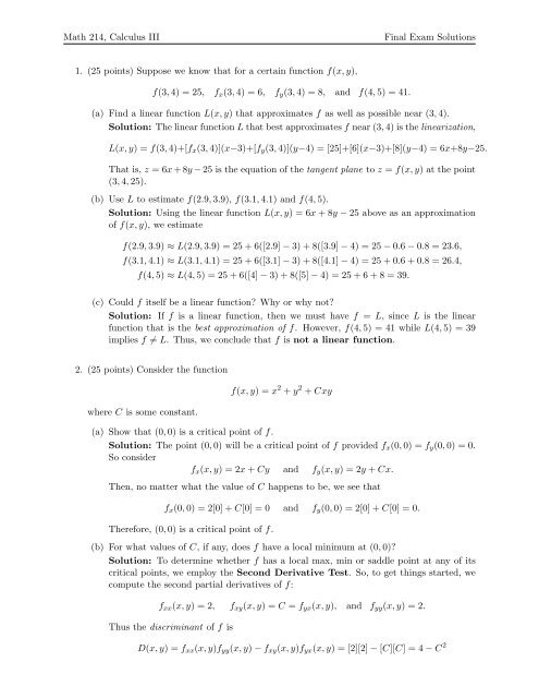
<strong>1.</strong> (<strong>25</strong> <strong>points</strong>) <strong>Suppose</strong> we know that for a certain function f(x, y),<br />
f(3, 4) = <strong>25</strong>, f x (3, 4) = 6, f y (3, 4) = 8, and f(4, 5) = 4<strong>1.</strong><br />
(a) Find a linear function L(x, y) that approximates f as well as possible near (3, 4).<br />
Solution: The linear function L that best approximates f near (3, 4) is the linearization,<br />
L(x, y) = f(3, 4)+[f x (3, 4)](x−3)+[f y (3, 4)](y−4) = [<strong>25</strong>]+[6](x−3)+[8](y−4) = 6x+8y−<strong>25</strong>.<br />
That is, z = 6x + 8y − <strong>25</strong> is the equation of the tangent plane to z = f(x, y) at the point<br />
(3, 4, <strong>25</strong>).<br />
(b) Use L to estimate f(2.9, 3.9), f(3.1, 4.1) and f(4, 5).<br />
Solution: Using the linear function L(x, y) = 6x + 8y − <strong>25</strong> above as an approximation<br />
of f(x, y), we estimate<br />
f(2.9, 3.9) ≈ L(2.9, 3.9) = <strong>25</strong> + 6([2.9] − 3) + 8([3.9] − 4) = <strong>25</strong> − 0.6 − 0.8 = 23.6,<br />
f(3.1, 4.1) ≈ L(3.1, 4.1) = <strong>25</strong> + 6([3.1] − 3) + 8([4.1] − 4) = <strong>25</strong> + 0.6 + 0.8 = 26.4,<br />
f(4, 5) ≈ L(4, 5) = <strong>25</strong> + 6([4] − 3) + 8([5] − 4) = <strong>25</strong> + 6 + 8 = 39.<br />
(c) Could f itself be a linear function? Why or why not?<br />
Solution: If f is a linear function, then we must have f = L, since L is the linear<br />
function that is the best approximation of f. However, f(4, 5) = 41 while L(4, 5) = 39<br />
implies f ≠ L. Thus, we conclude that f is not a linear function.<br />
2. (<strong>25</strong> <strong>points</strong>) Consider the function<br />
where C is some constant.<br />
f(x, y) = x 2 + y 2 + Cxy<br />
(a) Show that (0, 0) is a critical point of f.<br />
Solution: The point (0, 0) will be a critical point of f provided f x (0, 0) = f y (0, 0) = 0.<br />
So consider<br />
f x (x, y) = 2x + Cy and f y (x, y) = 2y + Cx.<br />
Then, no matter what the value of C happens to be, we see that<br />
f x (0, 0) = 2[0] + C[0] = 0 and f y (0, 0) = 2[0] + C[0] = 0.<br />
Therefore, (0, 0) is a critical point of f.<br />
(b) For what values of C, if any, does f have a local minimum at (0, 0)?<br />
Solution: To determine whether f has a local max, min or saddle point at any of its<br />
critical <strong>points</strong>, we employ the Second Derivative Test. So, to get things started, we<br />
compute the second partial derivatives of f:<br />
f xx (x, y) = 2, f xy (x, y) = C = f yx (x, y), and f yy (x, y) = 2.<br />
Thus the discriminant of f is<br />
D(x, y) = f xx (x, y)f yy (x, y) − f xy (x, y)f yx (x, y) = [2][2] − [C][C] = 4 − C 2
<strong>Math</strong> <strong>214</strong>, <strong>Calculus</strong> <strong>III</strong><br />
<strong>Final</strong> <strong>Exam</strong> <strong>Solutions</strong><br />
for all <strong>points</strong> (x, y). Recall that if D(x, y) > 0, then all of the concavities of f at (x, y)<br />
agree (i.e., the graph of f is either concave up in all directions at (x, y) or it is concave<br />
down in all directions at (x, y)); if D(x, y) < 0, then there are at least two directions<br />
in one of which the graph of f is concave up and in the other it is concave down (i.e.,<br />
the concavities don’t all agree at (x, y)); if D(x, y) = 0, then the Second Derivative Test<br />
doesn’t know what to do.<br />
Let’s first address the possibility of D = 0: i.e., C 2 = 4. Then C = ±2, so<br />
f(x, y) = x 2 + y 2 + 2xy = (x + y) 2 or f(x, y) = x 2 + y 2 − 2xy = (x − y) 2 .<br />
The graph of either of these functions is a parabolic cylinder whose vertex is along the<br />
line x+y = 0 (when C = 2) of along the line x−y = 0 (when C = −2) and the parabolas<br />
are all opening up. So, as (0, 0) is on the vertex line for these parabolic cylinders and<br />
the parabolas in the cylinder all open up, (0, 0) is a local minimum of f when C = ±2.<br />
Now consider the situation when the Second Derivative Test will be conclusive, i.e.,<br />
D ≠ 0. In order for f to have a minimum at (0, 0), first of all the discriminant must be<br />
positive, so 4 − C 2 > 0 which implies that C 2 < 4 so −2 < C < 2. Then, so long as<br />
−2 < C < 2, (0, 0) will be a minimum of f provided that f xx (0, 0) > 0, since this implies<br />
that the graph of f is concave up in all directions at (0, 0). But f xx (0, 0) = 2 > 0, so<br />
the graph of f is concave up and (0, 0) is a minimum (with f(0, 0) = 0 as the minimum<br />
value of f). Therefore, f has a local minimum at the point (0, 0) if<br />
−2 ≤ C ≤ 2.<br />
(c) For what values of C, if any, does f have a local maximum at (0, 0)?<br />
Solution: From the analysis in part (b), for f to have any chance to have a local<br />
maximum at (0, 0), we need D(0, 0) > 0, so −2 < C < 2, to ensure that all of the<br />
concavities of the graph of f agree at (0, 0) and we need f xx (0, 0) < 0 to imply that<br />
these concavities are all down to conclude that f has a local max at (0, 0). However,<br />
f xx (0, 0) = 2 > 0 is not less than zero. Therefore, there is<br />
for which f has a local maximum at (0, 0).<br />
no value of C<br />
(d) For what values of C, if any, does f have a saddle point at (0, 0)?<br />
Solution: Appealing to our work in part (b) again, we know that f will have a<br />
saddle point at (0, 0) so long as the discriminant is negative, as this will imply that<br />
the concavities in two different directions disagree with one another. Thus, we want<br />
D(0, 0) = 4 − C 2 < 0, i.e., 4 < C 2 . This inequality has the solution<br />
C < −2 or C > 2<br />
and either of these options will imply that f has a saddle point at (0, 0).<br />
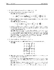
3. (<strong>25</strong> <strong>points</strong>) A flat circular plate has the shape of the region x 2 + y 2 ≤ <strong>1.</strong> The plate, including<br />
the boundary where x 2 + y 2 = 1, is heated so that the temperature at the point (x, y) is<br />
T (x, y) = x 2 + 2y 2 − x.<br />
Find the temperatures at the hottest and coldest <strong>points</strong> on the plate.
<strong>Math</strong> <strong>214</strong>, <strong>Calculus</strong> <strong>III</strong><br />
<strong>Final</strong> <strong>Exam</strong> <strong>Solutions</strong><br />
Solution: This is an extreme value problem with constraints, i.e., that we’re looking for the<br />
absolute maximum and absolute minimum values of the function T (x, y) = x 2 + 2y 2 − x on<br />
the region x 2 + y 2 ≤ <strong>1.</strong> So, to begin, we look for critical <strong>points</strong> of T in the interior of the<br />
plate, x 2 + y 2 < <strong>1.</strong> Thus, consider<br />
T x (x, y) = 2x − 1 = 0 =⇒ x = 1/2, T y (x, y) = 4y = 0 =⇒ y = 0<br />
Therefore, (1/2, 0) is the only critical point of the function T (x, y) and (1/2, 0) is within the<br />
interior of the plate, as (1/2) 2 + (0) 2 = 1/4 < <strong>1.</strong> Moreover, we have<br />
T xx = 2, T xy = 0 = T yx , T yy = 4 =⇒ D = [2][4] − [0] 2 = 8 > 0<br />
implies that (1/2, 0) is a local minimum of the function T since D > 0 implies all of the<br />
concavities agree at (1/2, 0) and T xx (1/2, 0) = 2 > 0 implies these concavities are all up,<br />
meaning that (1/2, 0, −1/4) is a local minimum point.<br />
Now we consider the boundary of the plate and search for extreme values subject to the<br />
constraint x 2 + y 2 = 1, i.e., y 2 = 1 − x 2 , so that we may write T in terms of just the variable<br />
x as<br />
T (x, ± √ 1 − x 2 ) = x 2 + 2(1 − x 2 ) − x = −x 2 − x + 2.<br />
Then T ′ (x) = −2x − 1, which is zero when x = −1/2, so y = ± √ 1 − (−1/2) 2 = ± √ 3/4.<br />
That is, T has “critical <strong>points</strong>” on the boundary, x 2 + y 2 = 1, at the <strong>points</strong> (−1/2, √ 3/4)<br />
and (−1/2, − √ 3/4), at which <strong>points</strong> T has the values<br />
T (−1/2, ± √ 3/4) = (−1/2) 2 + 2(± √ 3/4) 2 − (−1/2) = 1/4 + 2(3/4) + 1/2 = 9/4.<br />
So, from our analysis, the only possible <strong>points</strong> where absolute extreme values of T can occur<br />
are at the one interior point (1/2, 0), where T (1/2, 0) = −1/4, and at the two boundary<br />
<strong>points</strong> (−1/2, ± √ 3/4), where T (−1/2, ± √ 3/4) = 9/4. Since 9/4 > −1/4, we conclude that<br />
the temperature at the hottest point(s) on the plate is 9/4 = 2.<strong>25</strong>, which occurs at the two<br />
boundary <strong>points</strong> (−1/2, ± √ 3/4), and at the coldest point on the plate, i.e., at (1/2, 0), the<br />
temperature is T (1/2, 0) = −1/4 = −0.<strong>25</strong>.<br />
4. (<strong>25</strong> <strong>points</strong>) Consider the curve r(t) = 〈cos(t) + t sin(t), sin(t) − t cos(t)〉 defined for t > 0.<br />
(a) Find the velocity vector, v(t), for this curve.<br />
Solution: The velocity vector is v(t) = r ′ (t), so it is<br />
v(t) = 〈− sin(t) + t cos(t) + sin(t), cos(t) − t(− sin(t)) − cos(t)〉 = 〈t cos(t), t sin(t)〉.<br />
(b) Find the unit tangent vector, T(t), for this curve.<br />
Solution: The unit tangent vector is<br />
T(t) = 1<br />
|v(t)| v(t) = 1<br />
√ 〈t cos t, t sin t〉<br />
(t cos t) 2 + (t sin t) 2<br />
1<br />
= √<br />
t 2 (cos 2 t + sin 2 t) 〈t cos t, t sin t〉 = 1 〈t cos t, t sin t〉<br />
t<br />
= 〈cos t, sin t〉.
<strong>Math</strong> <strong>214</strong>, <strong>Calculus</strong> <strong>III</strong><br />
<strong>Final</strong> <strong>Exam</strong> <strong>Solutions</strong><br />
(c) Find the principal normal vector, N(t), for this curve.<br />
Solution: The principal normal vector is<br />
N(t) = 1<br />
|T ′ (t)| T′ (t) =<br />
1<br />
1<br />
√ 〈− sin t, cos t〉 = √ 〈− sin t, cos t〉 = 〈− sin t, cos t〉.<br />
(− sin t) 2 + (cos t) 2 1<br />
(d) Use your previous results together with the equation<br />
κN = dT<br />
ds = T′ (t)<br />
|r ′ (t)|<br />
to find the curvature κ for this curve.<br />
Solution: From part (a), we found that r ′ (t) = v(t) = 〈t cos(t), t sin(t)〉. In (b),<br />
we found T(t) = 〈cos t, sin t〉, so that T ′ (t) = 〈− sin t, cos t〉. In part (c), we found<br />
N(t) = 〈− sin t, cos t〉 = T ′ (t). Thus,<br />
κ = |κN(t)| =<br />
T ′ √ √<br />
(t)<br />
∣|r ′ (t)| ∣ = |T′ (t)| (− sin t)<br />
|r ′ (t)| = 2 + (cos t)<br />
√ 2 1<br />
(t cos t) 2 + (t sin t) = √ = 1 2 t 2 t .<br />
5. (<strong>25</strong> <strong>points</strong>) The graph y = f(x) in the xy-plane automatically has the parametrization x =<br />
x, y = f(x), and the vector formula r(x) = 〈x, f(x)〉. Using this formula, if f is a twicedifferentiable<br />
function of x, we can show<br />
κ(x) =<br />
|f ′′ (x)|<br />
[1 + (f ′ (x)) 2 ] 3/2 .<br />
(a) Use the formula for the curvature κ(x) above to find the curvature for the parabola<br />
y = x 2 .<br />
Solution: To find the curvature of the parabola y = x 2 , so that f(x) = x 2 is our<br />
function, we should find f ′ (x) = 2x and f ′′ (x) = 2. Then we have<br />
κ(x) =<br />
|f ′′ (x)|<br />
[1 + (f ′ (x)) 2 ] 3/2 = |2|<br />
[1 + (2x) 2 ] 3/2 = 2<br />
[1 + 4x 2 ] 3/2 .<br />
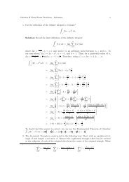
(b) We find the total curvature of the portion of a smooth curve that runs from s = s 0 to<br />
s = s 1 (s 1 > s 0 ) by integrating κ from s 0 to s 1 . If the curve has some other parameter,<br />
say t, then the total curvature is<br />
K =<br />
∫ s1<br />
s 0<br />
κ ds =<br />
∫ t1<br />
t 0<br />
κ ds<br />
dt dt = ∫ t1<br />
t 0<br />
κ|v(t)| dt,<br />
where t 0 and t 1 correspond to s 0 and s 1 .<br />
Find the total curvature of the parabola y = x 2 , −∞ < x < ∞.<br />
Solution: The parametrization of the parabola is, as described in the introduction to<br />
this problem, given by<br />
r(x) = 〈x, f(x)〉 = 〈x, x 2 〉.
<strong>Math</strong> <strong>214</strong>, <strong>Calculus</strong> <strong>III</strong><br />
<strong>Final</strong> <strong>Exam</strong> <strong>Solutions</strong><br />
Using this together with the formula for the total curvature K and our answer for κ(x)<br />
in part (a) above, we find<br />
K =<br />
=<br />
=<br />
=<br />
∫ ∞<br />
−∞<br />
∫ ∞<br />
−∞<br />
∫ ∞<br />
−∞<br />
∫ ∞<br />
−∞<br />
∫ 0<br />
κ(x)|v(x)| dx<br />
[<br />
]<br />
2<br />
[1 + 4x 2 ] 3/2 |〈1, 2x〉| dx<br />
[<br />
]<br />
2 √(1)<br />
[1 + 4x 2 ] 3/2 2 + (2x) 2 dx<br />
2<br />
1 + 4x 2 dx<br />
∫<br />
2<br />
∞<br />
=<br />
−∞ 1 + 4x 2 dx + 0<br />
[∫ 0<br />
= lim<br />
a→−∞<br />
= lim<br />
a→−∞<br />
= lim<br />
a→−∞<br />
= lim<br />
a→−∞<br />
a<br />
[∫ 0<br />
a<br />
[∫ 0<br />
x=a<br />
[∫ 0<br />
x=a<br />
[∫ 0<br />
= lim<br />
a→−∞<br />
x=a<br />
2<br />
1 + 4x 2 dx<br />
] [∫<br />
2<br />
b<br />
1 + 4x 2 dx + lim<br />
b→∞ 0<br />
] [∫<br />
2 dx<br />
b<br />
1 + (2x) 2 + lim<br />
b→∞ 0<br />
] [∫<br />
du<br />
b<br />
1 + u 2 + lim<br />
b→∞ x=0<br />
sec 2 ]<br />
θ dθ<br />
1 + (tan θ) 2 + lim<br />
]<br />
dθ<br />
[∫ b<br />
+ lim<br />
b→∞ x=0<br />
b→∞<br />
[∫ b<br />
]<br />
dθ<br />
]<br />
2<br />
1 + 4x 2 dx<br />
]<br />
2 dx<br />
1 + (2x) 2<br />
]<br />
du<br />
1 + u 2<br />
x=0<br />
sec 2 ]<br />
θ dθ<br />
1 + (tan θ) 2<br />
= lim<br />
a→−∞ [θ]0 x=a + lim<br />
b→∞ [θ]b x=0<br />
[<br />
= lim tan −1 (u) ] 0<br />
a→−∞<br />
x=a + lim<br />
[<br />
tan −1 (u) ] b<br />
b→∞<br />
x=0<br />
[<br />
= lim tan −1 (2x) ] 0<br />
a→−∞<br />
a + lim<br />
[<br />
tan −1 (2x) ] 0<br />
b→∞<br />
a<br />
[<br />
= lim tan −1 (0) − tan −1 (2a) ] [<br />
+ lim tan −1 (2b) − tan −1 (0) ]<br />
a→−∞<br />
b→∞<br />
[ (<br />
= 0 − − π )] [( π<br />
) ]<br />
+ − 0 = π.<br />
2 2<br />
6. (<strong>25</strong> <strong>points</strong>) <strong>Suppose</strong> f(x, y, z) is differentiable in a region whose interior contains a smooth<br />
curve<br />
C : r(t) = 〈g(t), h(t), k(t)〉.<br />
Consider the function f(r(t)) = f (g(t), h(t), k(t)) of the variable t.<br />
(a) Use the Chain Rule to find df<br />
dt .<br />
Solution: By the Chain Rule, we have<br />
(b) Show that df<br />
dt = ∇f · r′ (t).<br />
df<br />
dt = ∂f dx<br />
∂x dt + ∂f dy<br />
∂y dt + ∂f dz<br />
∂z dt = [f x]g ′ (t) + [f y ]h ′ (t) + [f z ]k ′ (t).
<strong>Math</strong> <strong>214</strong>, <strong>Calculus</strong> <strong>III</strong><br />
<strong>Final</strong> <strong>Exam</strong> <strong>Solutions</strong><br />
Solution: The gradient of f, ∇f is<br />
∇f = 〈f x , f y , f z 〉<br />
while<br />
Hence,<br />
r ′ (t) = 〈g ′ (t), h ′ (t), k ′ (t)〉.<br />
∇f · r ′ (t) = 〈f x , f y , f z 〉 · 〈g ′ (t), h ′ (t), k ′ (t)〉 = [f x ]g ′ (t) + [f y ]h ′ (t) + [f z ]k ′ (t) = df<br />
dt .<br />
(c) <strong>Suppose</strong> P 0 is a point on C where f has a local maximum or a local minimum relative<br />
to its values on C. Use part (b) to explain why ∇f is orthogonal to C at P 0 .<br />
Solution: As a function of t, if f(r(t)) has either a local max or min at P 0 , then we<br />
must have df<br />
df<br />
= 0. However, by part (b),<br />
dt dt = ∇f · r′ (t), so ∇f · r ′ (t) = 0 at P 0 . But<br />
two vectors are orthogonal if and only if their dot product is zero, so we conclude that<br />
∇f is orthogonal to r ′ (t) at P 0 . Yet, r ′ (t) is a tangent vector to the curve C at the point<br />
P 0 , so ∇f is orthogonal to the curve C at P 0 as claimed.<br />
7. (<strong>25</strong> <strong>points</strong>) Find the average value of f(x, y) = x 2 + y 2 over each of the following regions:<br />
(a) the square 0 ≤ x ≤ 1, 0 ≤ y ≤ <strong>1.</strong><br />
Solution: The average value of f over a region D is defined to be f ave =<br />
Thus, as the area of the square A : 0 ≤ x ≤ 1, 0 ≤ y ≤ 1 is 1, we have<br />
f ave = 1 ∫∫<br />
∫ 1 ∫ 1<br />
(x 2 + y 2 ) dA = (x 2 + y 2 ) dy dx =<br />
[1] A<br />
x=0 y=0<br />
∫ 1<br />
[<br />
= x 2 + 1 ] [ 1<br />
dx =<br />
x=0 3 3 x3 + 1 ] 1<br />
3 x = 1<br />
x=0<br />
3 + 1 3 = 2 3 .<br />
∫ 1<br />
x=0<br />
1 ∫∫<br />
area(D)<br />
D<br />
f(x, y) dA.<br />
[<br />
x 2 y + 1 3 y3 ] 1<br />
y=0<br />
(b) the square 0 ≤ x ≤ a, 0 ≤ y ≤ a, where a > 0.<br />
Solution: On the square B : 0 ≤ x ≤ a, 0 ≤ y ≤ a, whose area is area(B) = a 2 , we have<br />
f ave = 1 ∫∫<br />
[a 2 (x 2 + y 2 ) dA = 1 ∫ a ∫ a<br />
] B<br />
a 2 (x 2 + y 2 ) dy dx = 1 ∫ a<br />
[<br />
x=0 y=0<br />
a 2 x 2 y + 1 ] a<br />
x=0 3 y3 y=0<br />
= 1 a 2 ∫ a<br />
x=0<br />
[ax 2 + a3<br />
3<br />
]<br />
dx = 1 [ ] a a<br />
a 2 3 x3 + a3<br />
3 x = 1 [ a<br />
4<br />
0<br />
a 2 3 + a4<br />
3<br />
]<br />
= 2 3 a2 .<br />
dx<br />
dx<br />
(c) the disc x 2 + y 2 ≤ a 2 , where a > 0.<br />
Solution: On the disc D : x 2 + y 2 ≤ a 2 , whose area is area(D) = πa 2 , we have<br />
f ave = 1 ∫∫<br />
[πa 2 ]<br />
= 1<br />
πa 2 ∫ 2π<br />
θ=0<br />
(x 2 + y 2 ) dA = 1 ∫ 2π<br />
D<br />
πa 2 θ=0<br />
[ ] 1<br />
4 a4 dθ = 1 [ ] a<br />
4 2π<br />
πa 2 4 θ<br />
θ=0<br />
∫ a<br />
r=0<br />
(r 2 ) r dr dθ = 1<br />
πa 2 ∫ 2π<br />
= 1<br />
πa 2 [ a<br />
4<br />
4 (2π) ]<br />
= a2<br />
2 .<br />
θ=0<br />
[ 1<br />
4 r4 ] a<br />
r=0<br />
dθ
<strong>Math</strong> <strong>214</strong>, <strong>Calculus</strong> <strong>III</strong><br />
<strong>Final</strong> <strong>Exam</strong> <strong>Solutions</strong><br />
8. (<strong>25</strong> <strong>points</strong>) To celebrate the beginning of spring break, you treat yourself to an ice cream cone.<br />
Upon examination, you recognize that the ice cream cone fills the region in space bounded<br />
by the top half of the sphere<br />
x 2 + y 2 + (z − 1) 2 = 1<br />
above and by the cone<br />
z = √ x 2 + y 2<br />
below. Find the volume of your ice cream cone.<br />
[Hint: First integrate with respect to z, and then convert to polar coordinates.]<br />
Solution: The top half of the sphere x 2 + y 2 + (z − 1) 2 = 1 is obtained by solving for z<br />
by taking the positive square root (the negative square root yields the bottom half of the<br />
sphere), so the top of the ice cream cone is<br />
(z − 1) 2 = 1 − x 2 − y 2 =⇒ z − 1 = √ 1 − x 2 − y 2 =⇒ z = 1 + √ 1 − x 2 − y 2 .<br />
Now the top half of this sphere and the cone intersect when we have √ x 2 + y 2 = z =<br />
1 + √ 1 − x 2 − y 2 , i.e.,<br />
√<br />
x 2 + y 2 − √ 1 − x 2 − y 2 = 1 =⇒ (x 2 + y 2 ) − 2 √ x 2 + y 2√ 1 − x 2 − y 2 + (1 − x 2 − y 2 ) = 1<br />
=⇒ −2 √ x 2 + y 2√ 1 − x 2 − y 2 = 0<br />
=⇒ x 2 + y 2 = 0 or x 2 + y 2 = <strong>1.</strong><br />
The first option, x 2 + y 2 = 0, is where the bottom half of the sphere and the cone intersect at<br />
the vertex of the cone, so we discard this option (as we are only concerned with the top half<br />
of the cone, so that z ≥ 1), which means that the region in the xy-plane that is the shadow<br />
of the ice cream cone is the disc D : x 2 + y 2 ≤ 1, which is given by 0 ≤ r ≤ 1, 0 ≤ θ ≤ 2π in<br />
polar coordinates. Therefore, the volume of the ice cream cone is<br />
∫∫∫<br />
V =<br />
∫∫<br />
=<br />
=<br />
=<br />
=<br />
D<br />
∫ 2π ∫ 1<br />
θ=0<br />
∫ 2π<br />
θ=0<br />
∫ 2π<br />
∫∫<br />
dV =<br />
D<br />
[(1 + √ 1 − x 2 − y 2 )<br />
−<br />
r=0<br />
[<br />
1<br />
∫<br />
√<br />
1+ 1−x 2 −y 2 ∫∫<br />
√ dz dA =<br />
z= x 2 +y 2 D<br />
(√ )]<br />
x 2 + y 2 dA<br />
[1 + √ 1 − r 2 − √ r 2 ]<br />
r dr dθ =<br />
] 1<br />
2 r2 − 1 (1 − r 2 ) 3/2<br />
− 1 2 3/2 3 r3 dθ =<br />
r=0<br />
[ ] [ ] 1 1 2π<br />
dθ =<br />
θ=0 2 2 θ = π.<br />
0<br />
∫ 2π ∫ 1<br />
[z] 1+√ 1−x 2 −y 2<br />
z= √ x 2 +y 2 dA<br />
θ=0 r=0<br />
∫ 2π<br />
[<br />
r + r √ 1 − r 2 − r 2] dr dθ<br />
θ=0<br />
[( 1<br />
2 − 0 − 1 3<br />
So, along with your ice cream, you get to enjoy a little π. Happy “Pi Day.”<br />
9. (<strong>25</strong> <strong>points</strong>) Let F(x, y) = 〈3x 2 y 2 , 2x 3 y〉.<br />
)<br />
−<br />
(0 − 1 )]<br />
3 − 0<br />
(a) Show that F is a conservative vector field.<br />
Solution: First of all, we observe that F is defined on all of R 2 , which is open and simply<br />
connected. So, to prove that F is conservative, it is enough to prove that P y = Q x , where<br />
P = 3x 2 y 2 =⇒ P y = 6x 2 y<br />
Q = 2x 3 y =⇒ Q x = 6x 2 y<br />
dθ
<strong>Math</strong> <strong>214</strong>, <strong>Calculus</strong> <strong>III</strong><br />
<strong>Final</strong> <strong>Exam</strong> <strong>Solutions</strong><br />
As we can see above, the vector field F = 〈P, Q〉 satisfies P y = Q x , so F is conservative.<br />
(b) Find a potential function for F.<br />
Solution: By the Fundamental Theorem for Line Integrals, we know that a potential<br />
function for F exists, i.e., there is a scalar function f(x, y) with F = ∇f. In particular,<br />
this means that f x = P , so<br />
∫ ∫ [3x<br />
f(x, y) = P dx = 2 y 2] dx = x 3 y 2 + C(y)<br />
for some function C(y), which is constant with respect to x. From this form of f, we can<br />
determine C(y) by comparing f y = 2x 3 y + C ′ (y) with Q = 2x 3 y. The equality f y = Q<br />
then implies that C ′ (y) = 0, so that C(y) = K for some constant K (i.e., K is a number<br />
and is not a function of either x or y). Thus<br />
is the generic potential function of F.<br />
f(x, y) = x 3 y 2 + K<br />
(c) Let C be the curve parametrized by r(t) = 〈3t 2 + 1, 2t〉, 0 ≤ t ≤ <strong>1.</strong> Find ∫ C F · dr.<br />
Solution: By the Fundamental Theorem for Line Integrals,<br />
∫<br />
F · dr = f(r(1)) − f(r(0)) = f(4, 2) − f(1, 0) = [(4) 3 (2) 2 ] − [(1) 3 (0) 2 ] = <strong>25</strong>6.<br />
C<br />
10. (<strong>25</strong> <strong>points</strong>) Evaluate the line integral ∮ C y2 dx+x 2 dy, where C is the circle x 2 +y 2 = 4 using:<br />
(a) the parametrization r(t) = 〈2 cos(t), 2 sin(t)〉, 0 ≤ t ≤ 2π, of C.<br />
Solution: The vector field F corresponding to the differential form y 2 dx + x 2 dy is<br />
F(x, y) = 〈y 2 , x 2 〉, so ∮ C y2 dx + x 2 dy = ∮ C<br />
F · dr. Computing the latter line integral<br />
using the parametrization r(t), we obtain<br />
∮<br />
C<br />
F · dr =<br />
=<br />
∫ 2π<br />
0<br />
∫ 2π<br />
0<br />
〈4 sin 2 t, 4 cos 2 t〉 · 〈−2 sin t, 2 cos t〉 dt =<br />
∫ 2π<br />
8(1 − cos 2 t)[− sin t] + 8(1 − sin 2 t)[cos t] dt<br />
[ (<br />
= 8 cos t − 1 ) (<br />
3 cos3 t + 8 sin t − 1 )] 2π<br />
3 sin3 t<br />
0<br />
[(<br />
= 8 1 − 1 ) ] [(<br />
+ (0 − 0) − 8 1 − 1 ) ]<br />
+ (0 − 0)<br />
3<br />
3<br />
0<br />
−8 sin 3 t + 8 cos 3 t dt<br />
= 0.<br />
(b) Green’s Theorem.<br />
Solution: As in part (a), we have ∮ C y2 dx + x 2 dy = ∮ C F · dr, where F(x, y) = 〈y2 , x 2 〉.<br />
By Green’s Theorem, which applies to this problem since F is defined on all of R 2 (which<br />
is an open, simply connected domain) and the circle C is both simple and closed, we
<strong>Math</strong> <strong>214</strong>, <strong>Calculus</strong> <strong>III</strong><br />
<strong>Final</strong> <strong>Exam</strong> <strong>Solutions</strong><br />
have<br />
∮ ∫∫<br />
F · dr =<br />
C<br />
=<br />
=<br />
( ∂Q<br />
∂x − ∂P ) ∫∫<br />
dA =<br />
∂y<br />
R<br />
∫ 2π ∫ 2<br />
θ=0<br />
∫ 2π<br />
= 16<br />
3<br />
r=0<br />
θ=0<br />
∫ 2π<br />
R<br />
(2x − 2y) dA<br />
(2r cos θ − 2r sin θ) r dr dθ =<br />
[ ] 2 2<br />
(cos θ − sin θ)<br />
3 r3 dθ =<br />
r=0<br />
θ=0<br />
(cos θ − sin θ) dθ = 16 3<br />
∫ 2π<br />
θ=0<br />
∫ 2π ∫ 2<br />
θ=0<br />
r=0<br />
2r 2 (cos θ − sin θ) dr dθ<br />
[ ] 16<br />
(cos θ − sin θ) dθ<br />
3<br />
[sin θ + cos θ]2π<br />
θ=0 = 16 [(0 + 1) − (0 + 1)] = 0.<br />
3