Math 214, Calculus III Test 2 — Solutions 1. (20 points) Consider the ...
Math 214, Calculus III Test 2 — Solutions 1. (20 points) Consider the ...
Math 214, Calculus III Test 2 — Solutions 1. (20 points) Consider the ...

Create successful ePaper yourself
Turn your PDF publications into a flip-book with our unique Google optimized e-Paper software.
<strong>Math</strong> <strong>214</strong>, <strong>Calculus</strong> <strong>III</strong><br />
<strong>Test</strong> 2 <strong>—</strong> <strong>Solutions</strong><br />
<strong>1.</strong> (<strong>20</strong> <strong>points</strong>) <strong>Consider</strong> <strong>the</strong> function<br />
f(x,y) = 2xy − 3y 2<br />
near <strong>the</strong> point P(5,5).<br />
(a) Find <strong>the</strong> rate of change of f(x,y) at P in <strong>the</strong> direction of <strong>the</strong> vector v = 〈4,3〉.<br />
Solution: The rates of change of f at P are measured by <strong>the</strong> directional derivatives,<br />
D u f(P). Now D u f(P) = ∇f(P) · u, where<br />
∇f(P) = 〈f x (P),f y (P)〉 = 〈 2y| (5,5) ,2x − 6y| (5,5) 〉 = 〈 10, −<strong>20</strong> 〉.<br />
Now, we need to find <strong>the</strong> unit vector u in <strong>the</strong> direction of v = 〈4,3〉, which is<br />
u = v<br />
|v| = 〈4,3〉<br />
√<br />
(4) 2 + (3) 2 = 〈 4 5 , 3 5 〉.<br />
Thus, <strong>the</strong> rate of change of f(x,y) at P in <strong>the</strong> specified direction is<br />
D u f(P) = ∇f(P) · u = 〈 10, −<strong>20</strong> 〉 · 〈 4 5 , 3 5<br />
〉 = (10)(4/5) + (−<strong>20</strong>)(3/5) = 8 − 12 = −4.<br />
(b) In which direction does <strong>the</strong> function f(x,y) increase most rapidly at P?<br />
Solution: The directional derivative of f at P will be largest when ∇f(P) and u point<br />
in <strong>the</strong> same direction, since D u f(P) = ∇f(P) · u = |∇f(P)||u|cos θ = |∇f(P)|cos θ,<br />
where θ is <strong>the</strong> angle between ∇f(P) and u. Now ∇f(P) = 〈 10, −<strong>20</strong> 〉, so we want u to<br />
be <strong>the</strong> unit vector in this direction, i.e.,<br />
u =<br />
〈 10, −<strong>20</strong> 〉<br />
|〈 10, −<strong>20</strong> 〉| = 〈 10, −<strong>20</strong> 〉 〈 10, −<strong>20</strong> 〉<br />
√ =<br />
(10) 2 + (−<strong>20</strong>) 2 10 √ = 〈<br />
5<br />
1<br />
√ , √ −2 〉. 5 5<br />
(c) Is <strong>the</strong>re a direction u in which <strong>the</strong> rate of change of f(x,y) at P equals −25? Give<br />
reasons for your answer.<br />
Solution: We know that −|∇f(P)| ≤ D u f(P) ≤ |∇f(P)| for all directions u, so let’s<br />
compute<br />
|∇f(P)| = |〈10, −<strong>20</strong>〉| = √ (10) 2 + (−<strong>20</strong>) 2 = 10 √ 5 ≈ 22.36<br />
Thus, it is impossible to find a direction in which <strong>the</strong> rate of change of f(x,y) at P is<br />
equal to −25 since −25 < −|∇f(P)| ≈ −22.36.<br />
2. (30 <strong>points</strong>) <strong>Consider</strong> <strong>the</strong> surfaces S 1 and S 2 , given by <strong>the</strong> equations<br />
S 1 : x 3 + 3x 2 y 2 + y 3 + 4xy − z 2 = 0 and S 2 : x 2 + y 2 + z 2 = 11,<br />
and <strong>the</strong> point P(1,1,3), which is on both surfaces.<br />
(a) Find <strong>the</strong> equation of <strong>the</strong> tangent plane to S 1 at P.<br />
Solution: To know <strong>the</strong> equation of <strong>the</strong> tangent plane to S 1 at P, we need a point (i.e., P<br />
itself) and a vector perpendicular to S 1 at P. Here’s where <strong>the</strong> gradient comes in, as ∇f
<strong>Math</strong> <strong>214</strong>, <strong>Calculus</strong> <strong>III</strong><br />
<strong>Test</strong> 2 <strong>—</strong> <strong>Solutions</strong><br />
is perpendicular to <strong>the</strong> level surface of <strong>the</strong> function f(x,y,z) = x 3 +3x 2 y 2 +y 3 +4xy −z 2<br />
(for S 1 is given by f(x,y,z) = 0). Now we calculate<br />
so<br />
∇f = 〈 3x 2 + 6xy 2 + 4y,6x 2 y + 3y 2 + 4x, −2z 〉<br />
∇f(P) = 〈 3[1] 2 + 6[1][1] 2 + 4[1],6[1] 2 [1] + 3[1] 1 + 4[1], −2[3] 〉 = 〈 13,13, −6 〉.<br />
Hence <strong>the</strong> equation for <strong>the</strong> tangent plane, T 1 , to S 1 at P is<br />
[13](x − 1) + [13](y − 1) + [−6](z − 3) = 0 or 13x + 13y − 6z = 8.<br />
(b) Find <strong>the</strong> equation of <strong>the</strong> tangent plane to S 2 at P.<br />
Solution: As above, <strong>the</strong> equation for <strong>the</strong> tangent plane to S 2 at P requires a point (i.e.,<br />
P itself) and a vector perpendicular to S 2 at P. Here’s where <strong>the</strong> gradient comes in, as<br />
∇g is perpendicular to <strong>the</strong> level surface of <strong>the</strong> function g(x,y,z) = x 2 + y 2 + z 2 (for S 2<br />
is given by g(x,y,z) = 11). Now we calculate<br />
∇g = 〈 2x,2y,2z 〉 so ∇g(P) = 〈 2[1],2[1],2[3] 〉 = 〈 2,2,6 〉.<br />
Hence <strong>the</strong> equation for <strong>the</strong> tangent plane, T 2 , to S 2 at P is<br />
[2](x − 1) + [2](y − 1) + [6](z − 3) = 0 or x + y + 3z = 1<strong>1.</strong><br />
(c) Find <strong>the</strong> parametric equations for <strong>the</strong> line of intersection of <strong>the</strong> tangent planes in parts<br />
(a) and (b).<br />
Solution: To find <strong>the</strong> line tangent to <strong>the</strong> curve of intersection of S 1 and S 2 at P, which<br />
must <strong>the</strong>n be tangent to S 1 at P as well as to S 2 at P, we can quickly see that what we<br />
really are after is <strong>the</strong> line of intersection of <strong>the</strong> two planes from parts (b) and (c) above.<br />
So we need a direction for this line and a point on it. By definition, essentially, P is<br />
that point, and <strong>the</strong> direction will have to be a direction that is both in T 1 and in T 2 , so<br />
it is perpendicular to both <strong>the</strong> normal vector n 1 = 〈13,13, −6〉 to T 1 and to <strong>the</strong> normal<br />
vector n 2 = 〈2,2,6〉 to T 2 . We find such a vector using <strong>the</strong> cross product,<br />
⃗i ⃗j ⃗ k<br />
n 1 × n 2 = 〈13,13, −6〉 × 〈2,2,6〉 =<br />
13 13 −6<br />
= 〈90, −90,0〉.<br />
∣ 2 2 6 ∣<br />
Thus, <strong>the</strong> parametric equations for <strong>the</strong> line tangent to both surfaces S 1 and S 2 at <strong>the</strong><br />
point P are<br />
x = 1 + 90t, y = 1 − 90t, z = 3.<br />
[Note: This is <strong>the</strong> line tangent to <strong>the</strong> curve of intersection of <strong>the</strong> surfaces, S 1 and S 2 ,<br />
at <strong>the</strong> point P.]<br />
3. (10 <strong>points</strong>) Find <strong>the</strong> limit of f as (x,y) → (0,0) or show that <strong>the</strong> limit does not exist:<br />
f(x,y) =<br />
y2<br />
x 2 + y 2
<strong>Math</strong> <strong>214</strong>, <strong>Calculus</strong> <strong>III</strong><br />
<strong>Test</strong> 2 <strong>—</strong> <strong>Solutions</strong><br />
Solution: Let’s rewrite <strong>the</strong> function using polar coordinates, r and θ, and recognize that this<br />
limit will correspond to letting r → 0. Now<br />
y 2 (r sin θ)2<br />
x 2 =<br />
+ y2 r 2<br />
= r2 sin 2 θ<br />
r 2 = sin 2 θ,<br />
which clearly depends on <strong>the</strong> value of θ, even as r → 0. So <strong>the</strong> limit does not exist.<br />
We can also show this by comparing <strong>the</strong> value of <strong>the</strong> limit along two different lines, y = m 1 x<br />
and y = m 2 x for different slopes, m 1 and m 2 . For efficiency, let’s consider all lines y = mx,<br />
so (x,y) → (0,0) along y = mx is accomplished by letting x → 0 and evaluating<br />
lim<br />
x→0y=mx<br />
(mx) 2<br />
x 2 + (mx) 2 =<br />
lim<br />
x→0y=mx<br />
m 2 x 2<br />
x 2 (1 + m 2 ) =<br />
lim<br />
x→0y=mx<br />
m 2<br />
1 + m 2 = m2<br />
1 + m 2.<br />
(0)<br />
So, if m 1 = 0 and we let (x,y) → (0,0) along <strong>the</strong> line y = 0, <strong>the</strong> projected limit is<br />
2<br />
= 0.<br />
1+(0) 2<br />
However, when m 2 = 1 and (x,y) → (0,0) along <strong>the</strong> line y = x, we find that <strong>the</strong> projected<br />
(1)<br />
value of <strong>the</strong> limit is<br />
2<br />
= 1 1+(1) 2 2<br />
. Since <strong>the</strong>se differ, we conclude that <strong>the</strong> limit does not exist.<br />
4. (25 <strong>points</strong>) Find all <strong>the</strong> local maximum, local minimum, and saddle <strong>points</strong> of <strong>the</strong> function<br />
f(x,y) = 6x 2 − 2x 3 + 3y 2 + 6xy.<br />
Solution: We begin by finding <strong>the</strong> partial derivatives of f:<br />
f x (x,y) = 12x − 6x 2 + 6y and f y (x,y) = 6y + 6x.<br />
Setting f y = 0, we find that 6y = −6x, which we can now plug in to <strong>the</strong> equation f x = 0 to<br />
get<br />
12x − 6x 2 + [−6x] = 6x − 6x 2 = 6x(1 − x) = 0<br />
so x = 0 or x = <strong>1.</strong> When x = 0, <strong>the</strong> equation 6y = −6x tells us y = 0 as well so we find <strong>the</strong><br />
critical point (0,0) of f. When x = 1, 6y = −6x implies that y = −1 and (1, −1) is ano<strong>the</strong>r<br />
critical point of f.<br />
To test <strong>the</strong>se <strong>points</strong>, we compute <strong>the</strong> second order partial derivatives,<br />
f xx (x,y) = 12 − 12x, and f xy (x,y) = 6 = f yx (x,y), f yy (x,y) = 6.<br />
Therefore, <strong>the</strong> discriminent is<br />
D f (x,y) = [f xx ][f yy ] − [f xy ] 2 = [12 − 12x][6] − [6] 2 = 72 − 72x − 36 = 36 − 72x.<br />
We use this to test our first critical point:<br />
implies<br />
D f (0,0) = 36 − 72[0] = 36 > 0 and f xx (0,0) = 12 − 12[0] = 12 > 0<br />
f(0,0) = 0 is a local minimum value of f.<br />
Now, checking our o<strong>the</strong>r critical point, we find:<br />
D f (1, −1) = 36 − 72[1] = −36 < 0<br />
implies<br />
f(1, −1) = 1 is a saddle point of f.
<strong>Math</strong> <strong>214</strong>, <strong>Calculus</strong> <strong>III</strong><br />
<strong>Test</strong> 2 <strong>—</strong> <strong>Solutions</strong><br />
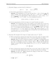
5. (40 <strong>points</strong>) <strong>Consider</strong> <strong>the</strong> function<br />
f(x,y) = 2x 2 − 4x + y 2 − 4y + 1<br />
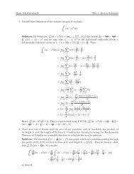
on <strong>the</strong> closed triangular region R bounded by <strong>the</strong> lines x = 0, y = 3 and y = x.<br />
(a) Find <strong>the</strong> absolute maximum and minimum values of f(x,y) on R.<br />
Solution: Let’s begin by drawing <strong>the</strong> region R described in <strong>the</strong> problem.<br />
4<br />
y = 3<br />
3<br />
2<br />
x = 0<br />
1<br />
y = x<br />
−1<br />
0 1 2 3 4<br />
So our strategy will be to first locate local extrema, <strong>the</strong>n to test each of <strong>the</strong> three<br />
boundary lines using <strong>Calculus</strong> I techniques.<br />
First, let’s identify <strong>the</strong> critical <strong>points</strong> of f. So we compute<br />
f x (x,y) = 4x − 4 and f y (x,y) = 2y − 4.<br />
Now f x (x,y) = 4x − 4 = 0 only when x = 1, and f y (x,y) = 2y − 4 = 0 only when y = 2,<br />
so (1,2) is <strong>the</strong> only critical point of <strong>the</strong> function f. Since we’re looking for absolute<br />
extrema, we don’t need to employ any Second Derivative <strong>Test</strong>s, but content ourselves to<br />
evaluate<br />
f(1,2) = 2[1] 2 − 4[1] + [2] 2 − 4[2] + 1 = −5.<br />
With <strong>the</strong> local extrema now determined, we restrict our attention to <strong>the</strong> boundaries. So<br />
consider<br />
f(0,y) = y 2 − 4y + 1 =⇒ f ′ (0,y) = 2y − 4 = 0 when y = 2.<br />
So, on <strong>the</strong> boundary x = 0, <strong>the</strong> “critical point” is at (0,2), so we record <strong>the</strong> value of at<br />
this point and <strong>the</strong> end<strong>points</strong> of this edge:<br />
f(0,0) = 1 and f(0,2) = −3 and f(0,3) = −2.<br />
Next, along <strong>the</strong> edge y = 3 we have<br />
f(x,3) = 2x 2 − 4x − 2 =⇒ f ′ (x,3) = 4x − 4 = 0 when x = <strong>1.</strong><br />
Hence, when y = 3, <strong>the</strong> “critical point” is at (1,3), so we record <strong>the</strong> values<br />
f(0,3) = −2 and f(1,3) = −4 and f(3,3) = 4.<br />
Finally, on <strong>the</strong> edge y = x, we have<br />
f(x,x) = 2x 2 −4x+[x] 2 −4[x]+1 = 3x 2 −8x+1 =⇒ f ′ (x,x) = 6x−8 = 0 when x = 4/3.
<strong>Math</strong> <strong>214</strong>, <strong>Calculus</strong> <strong>III</strong><br />
<strong>Test</strong> 2 <strong>—</strong> <strong>Solutions</strong><br />
So, on y = x, <strong>the</strong> only “critical point” is at (4/3,4/3), so we record<br />
f(0,0) = 1 and f(4/3,4/3) = − 13<br />
3<br />
and f(3,3) = 4.<br />
Therefore, <strong>the</strong> absolute maximum value of f(x,y) is f(3,3) = 4 and <strong>the</strong> absolute minimum<br />
value of f(x,y) is f(1,2) = −5.<br />
(b) Find <strong>the</strong> average value of f(x,y) on R.<br />
Solution: The average value of f(x,y) is<br />
f ave =<br />
1<br />
Area(R)<br />
∫∫<br />
R<br />
f(x,y) dA.<br />
While we could computer Area(R) as a double integral, it is clearly going to be easier<br />
to find this area by observing that R is a triangle of base b = 3 and height h = 3, so its<br />
area is<br />
Area(R) = 1 2 bh = 1 2 (3)(3) = 9 2 .<br />
Therefore, <strong>the</strong> average value of f(x,y) on <strong>the</strong> region R is<br />
∫∫<br />
1<br />
f ave =<br />
f(x,y) dA<br />
Area(R) R<br />
= 1 ∫∫<br />
[<br />
2x 2 − 4x + y 2 − 4y + 1 ] dA<br />
9/2 R<br />
= 2 ∫ 3<br />
∫ y [<br />
2x 2 − 4x + y 2 − 4y + 1 ] dxdy<br />
9 y=0 x=0<br />
= 2 ∫ 3<br />
[ 2x<br />
3<br />
y<br />
9 y=0 3 − 2x2 + xy 2 − 4xy + x]<br />
dy<br />
x=0<br />
= 2 ∫ 3<br />
[( ]<br />
2<br />
9 y=0 3 y3 − 2y 2 + y 3 − 4y 2 + y)<br />
− (0)<br />
= 2 [ 2 y 4<br />
] 3<br />
9 3 4 − 2y3 3 + y4<br />
4 − 4y3 3 + y2<br />
2<br />
y=0<br />
= 2 [( 81<br />
9 6 − 54<br />
3 + 81<br />
4 − 108<br />
3 + 9 ) ]<br />
− (0)<br />
2<br />
= 2 [ ] −189<br />
= − 21<br />
9 12 6 = −7 2 .<br />
dy<br />
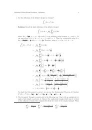
6. (25 <strong>points</strong>) Improper Double Integrals. <strong>Consider</strong> <strong>the</strong> integral<br />
∫ ∞ ∫ ∞<br />
0<br />
0<br />
1<br />
(1 + x 2 + y 2 ) 2 dxdy.<br />
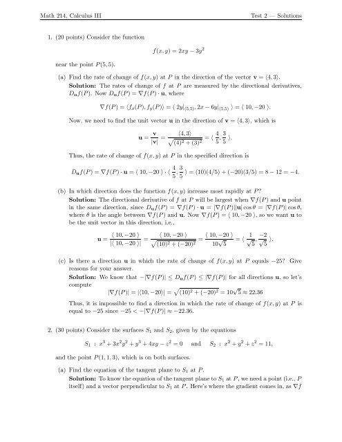
(a) First, sketch <strong>the</strong> region over which <strong>the</strong> integral is being taken.
<strong>Math</strong> <strong>214</strong>, <strong>Calculus</strong> <strong>III</strong><br />
<strong>Test</strong> 2 <strong>—</strong> <strong>Solutions</strong><br />
3<br />
2<br />
1<br />
−1<br />
−1<br />
1 2 3<br />
While I can’t (and don’t expect you to do so, ei<strong>the</strong>r) draw <strong>the</strong> entire first quadrant, that<br />
is <strong>the</strong> region over which <strong>the</strong> integral is being taken and which, I hope, you understand<br />
<strong>the</strong> illustration above to indicate.<br />
(b) Next, change <strong>the</strong> integral into an equivalent integral using polar coordinates, r and θ.<br />
Solution: Recall, first, that r 2 = x 2 + y 2 and that dxdy = dA = r dr dθ. Next, <strong>the</strong><br />
polar coordinates of <strong>points</strong> in <strong>the</strong> first quadrant are of <strong>the</strong> form (r,θ) with 0 ≤ r < ∞<br />
and 0 ≤ θ ≤ π 2<br />
, so <strong>the</strong> integral we are given is equivalent to <strong>the</strong> following polar integral:<br />
∫ ∞ ∫ ∞<br />
y=0<br />
x=0<br />
∫<br />
1<br />
π/2<br />
(1 + x 2 + y 2 ) 2 dxdy =<br />
θ=0<br />
∫ ∞<br />
r=0<br />
1<br />
(1 + r 2 r dr dθ.<br />
)<br />
2<br />
(c) Finally, evaluate <strong>the</strong> polar integral in part (b).<br />
Solution: Starting where we left off in part (b), we have<br />
∫ ∞ ∫ ∞<br />
0<br />
0<br />
∫<br />
1<br />
π/2<br />
(1 + x 2 + y 2 ) 2 dxdy =<br />
=<br />
=<br />
=<br />
=<br />
=<br />
θ=0<br />
∫ π/2<br />
θ=0<br />
∫ π/2<br />
θ=0<br />
∫ π/2<br />
θ=0<br />
∫ π/2<br />
θ=0<br />
= π 4 .<br />
∫ ∞<br />
1<br />
r=0 (1 + r 2 r dr dθ<br />
)<br />
2<br />
[ ∫ b<br />
]<br />
r<br />
lim<br />
b→∞ r=0 (1 + r 2 ) 2 dr dθ<br />
[<br />
1 (1 + r 2 ) −1 ] b<br />
lim<br />
dθ<br />
b→∞ 2 −1<br />
r=0<br />
[ ( −1<br />
lim<br />
b→∞ 2(1 + b 2 ) − −1<br />
2(1 + 0 2 )<br />
[ 1<br />
2]<br />
[ 1<br />
2 θ ] π/2<br />
θ=0<br />
dθ<br />
)]<br />
dθ