greenland climate network (gc-net) - HFT Stuttgart

More documents

Recommendations

Info

NASA Greenland Progress Report 15 3.3 Melt Anomalies on GIS Relation to North Atlantic Atmospheric Patterns and Arctic Sea Ice Concentration Due to its location in the North Atlantic storm track and its very shallow slope, the extent and volume of melt on Greenland are excellent indicators of <strong>climate</strong> change in the North Atlantic and the Arctic during the warm season. This study explores the relationships between inter-annual variability of melt in Greenland and regional scale atmospheric circulation as well as sea ice concentrations in the Arctic. Empirical orthogonal function (EOF) analysis is used to identify the dominant modes of variability in melt frequency in Greenland during the melt season. Melt frequency is defined as the total number of 25 km 2 passive microwave pixels that melted, summed over the entire melt season (April – October). A melting pixel is identified using the cross polarized gradient ratio (XPGR) applied to the passive microwave data record spanning 1979-2003 [Abdalati and Steffen, 1995]. 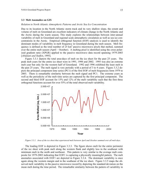Figure 3.3.1 depicts the total area-days of melt on the ice sheet for the past 25 years. The peak melt years for the entire ice sheet were in 1991, 1998 and 2002. 1995 was also an extreme melt year but only for the western half of Greenland. 1992 and 1996 exhibited the least melt in the past 25 years. The melt signal is very periodic with a period of 3 to 4 years. Figure 3.3.2 depicts the principal component time series (PC1) of the first EOF of melt frequencies form 1979 to 2003. There is remarkable similarity between the melt signal and PC1. The extreme years as well as the periodicity of the melt time series are captured by the first principal component. The second and third EOF account for 15% and 12% of the melt variability such that the first three orthogonal functions account for over 55% of the total observed melt variability. 2.50E+07 Area Melted (sq, km.) 2.00E+07 1.50E+07 1.00E+07 5.00E+06 0.00E+00 1979 1984 1989 1994 1999 2004 Year Figure 3.3.1. Area of the ice sheet that experienced melt between April and October summed over all melt days. The leading EOF is depicted in Figure 3.3.3. The figure shows melt for the entire perimeter of the ice sheet with peak melt along the western flank and slightly less in the southeast with minimum melt in the north and northeast. This pattern is very similar to the average melt composite for 1979-2003 indicating that EOF1 is capturing a physically meaningful pattern. The melt anomalies associated with EOF1 are depicted in Figure 3.3.4. The dominant variability is once again along the western margin and in the southeast of the ice sheet. Figure 3.3.5 maps the observed melt variability in the passive microwave record by depicting the standard deviation on the mean melt during the time period. The remarkable similarity between the pattern of variability in
NASA Greenland Progress Report 16 the observed melt and the melt anomalies associated with the first EOF indicate that the analysis is capturing a physically meaningful pattern such that rotating the principal component is not necessary. NCEP/NCAR reanalysis data was used to identify patterns of atmospheric pressure and temperature anomalies associated with the dominate mode of melt variability in Greenland. This was accomplished by regressing the time series of pressure and temperature anomalies from the reanalysis data onto PC1. The resulting pattern in the 750 hPa geopotential height anomalies is show in Figure 3.3.6. Two features in the plot stand clearly out. The first is the dome of high pressure over much of the Arctic Ocean extending south over Greenland. The second is the zonal pattern of closed high and low pressure contours between 50 and 60 N. In particular the low pressure center over Newfoundland in conjunction with the high pressure in the east Atlantic would support strong merridianal transport of warm southern air onto Greenland. Figure 3.3.6 indicates the possibility that the phase of zonal wave 3 is a determining factor in melt variability on the ice sheet and is being explored further. The surface temperature anomalies associated with melt EOF1 are shown in Figure 3.3.7. The map indicates Arctic wide, positive temperature anomalies consistent with merridianal advection of warm air into the region discussed above. 2 1.5 1991 1998 Stanard Deviations 1 0.5 0 -0.5 -1 -1.5 -2 1986 1992 1996 2002 1979 1981 1983 1985 1987 1989 Year Figure 3.3.2. Principal component time series of the leading EOF. Units are normalized to unit variance. The time series is 94% correlated with the total observed melt time series for 1979-2003. The sea ice concentration anomalies associated the leading melt EOF for Greenland are depicted in Figure 3.3.8. The pattern is nearly identical to that of the record sea ice anomalies observed during the last three Arctic summers. This intriguing result indicates that melt on the ice sheet may be responding to the same general circulation patterns responsible for recent extreme minimum sea ice concentrations. It further implies that the observed pattern of sea ice anomalies can be reconstructed considering only general atmospheric circulation patterns during the warm season. 1991 1993 1995 1997 1999 2001 2003
Page 1 and 2: VARIABILITY AND FORCING OF CLIMATE
Page 3 and 4: NASA Greenland Progress Report 2 1.
Page 7 and 8: NASA Greenland Progress Report 6 Da
Page 11 and 12: NASA Greenland Progress Report 10 T
Page 13 and 14: NASA Greenland Progress Report 12 3
Page 15: NASA Greenland Progress Report 14 s
Page 22 and 23: NASA Greenland Progress Report 21 S
Page 24 and 25: NASA Greenland Progress Report 23 D
Page 26 and 27: NASA Greenland Progress Report 25 p
Page 28 and 29: NASA Greenland Progress Report 27 F
Page 34 and 35: NASA Greenland Progress Report 33 R
Page 36: NASA Greenland Progress Report 35 S

greenland climate network (gc-net) - HFT Stuttgart

You also want an ePaper? Increase the reach of your titles

Delete template?

Save as template?