greenland climate network (gc-net) - HFT Stuttgart

VARIABILITY AND FORCING OF CLIMATE PARAMETERS
ON THE GREENLAND ICE SHEET:
GREENLAND CLIMATE NETWORK (GC-NET)
Konrad Steffen, Nicolas Cullen Russell Huff, John Maurer
University of Colorado at Boulder
Cooperative Institute for Research in Environmental Sciences
Division of Cryospheric and Polar Processes
Campus Box 216, Boulder CO 80309
and
Manfred Stober, Jörg Hepperle, Alexander Heise
Stuttgart University of Applied Sciences
Department of Surveying and Geoinformatics.
NAG5-10857
Annual Progress Report
to
National Aeronautics and Space Administration
February 2005
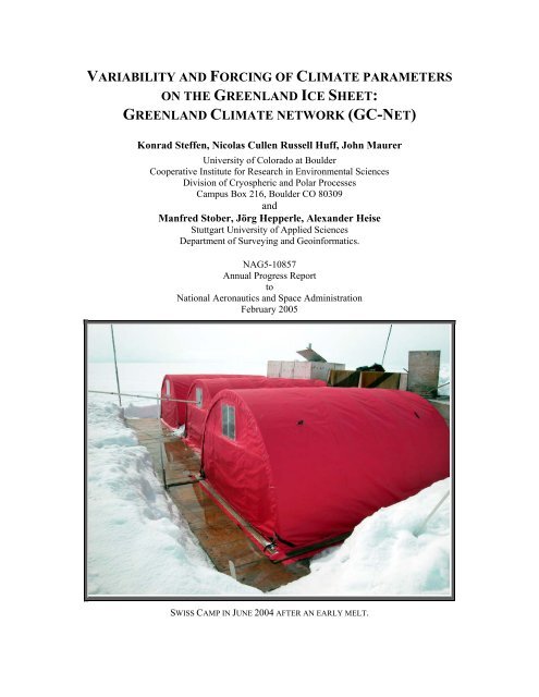
SWISS CAMP IN JUNE 2004 AFTER AN EARLY MELT.

TABLE OF CONTENTS
1. Activities ....................................................................................................................2
1.1 Summary of Highlights ................................................................................................. 2
1.2 Logistic Summary.......................................................................................................... 3
1.3 Personal ......................................................................................................................... 4
2. Greenland Climate Network (GC-Net)...................................................................5
2.1 Overview ....................................................................................................................... 5
2.2 GC-Net Citation List ..................................................................................................... 5
3. Applications and Results..........................................................................................8
3.1 Temperature and Radiation Climatology at Swiss Camp (1993-2004)......................... 8
3.2 The Melt Anomaly of 2002 – QuikSCAT and Passive Microwave Data.................... 11
3.2.1 Melt Detection from Passive Microwave............................................................ 11
3.2.2 Melt Detection from QuikSCAT....................................................................... 11
3.2.3 Statistical Analysis for Passive Microwave Derived Melt................................. 12
3.2.4 Recent melt observed by QuikSCAT................................................................. 13
3.3 Melt Anomalies on GIS............................................................................................... 15
Relation to North Atlantic Atmospheric Patterns and Arctic Sea Ice Concentration... 15
3.4 Geodetic Ground Measurements 2004 ........................................................................ 19
3.4.1 Geodetic Program............................................................................................... 19
3.4.2 Evaluation and Results........................................................................................ 20
3.4.3 Summary ............................................................................................................ 27
3.5 GPR Data Analysis...................................................................................................... 28
3.5.1 Data Processing.................................................................................................. 28
4. Proposed Field Activities and Research Objectives 2005 ...................................31
4.1 AWS Maintenance....................................................................................................... 31
4.2 GPS Network Maintenance ......................................................................................... 31
4.3 Ground Penetration Radar ........................................................................................... 31
4.4 NCEP Reanalysis, NAO, and Melt Extent .................................................................. 31
5. References................................................................................................................32
6. Publications and Presentations Supported by the Grant....................................34

NASA Greenland Progress Report 2
1.1 Summary of Highlights
1. Activities
Greenland Climate network (GC-Net)
• Ten AWS sites have been visited and serviced in spring 2004: ETH/CU, CP1, JAR1,
JAR2, JAR3, DYE-2, Saddle, NASA-SE, Petermann, Petermann ELA(Fig. 1.1).
• Quality control (QC) procedures have been refined and applied to all data, including data
collected during the 2003 field campaign.
• The satellite transmitted AWS raw data can now be processed and quality controlled with
IDL programs on Window 2000/XP computers.
• Results supported by this grant have been published in 15 peer-reviewed publications and
32 peer-reviewed publications made use of the GC-Net AWS data.
Applications and Results
• The mean annual temperature at Swiss Camp is -11.9° C over the ten-year time period
1991-2004.
• Summer month with above freezing mean temperatures occurred in 1995, and from
1997– 2004.
• The largest monthly mean net radiation At Swiss Camp was found in summer 1995 (> 40
W m -2 ) over the twelve-year time period 1993-2004, coincident with the time period with
minimum.
• The diurnal cycle of net radiation ranges between –80 W m -2 to 130 W m -2 for cloud-free
days.
• The twelve-year annual mean net radiation value –13.9 W m -2 , and for the winter month
November – February a negative mean flux density of –26.4 W m -2 was recorded.
• The annual mean temperature increased at Swiss Camp from -14.7º C (1991) to -10.8º
(2003), mean spring temperatures increased from -17.2º C to -13.6º C, and fall temperatures
show a similar trend from -13.8º C to -10.3º C for the 1991 to 2004 record.
• The largest increase of 6º C was observed for mean winter temperatures, ranging from -
25.3º C (1991) to -19.3º C (2003).
• The melt extent, defined as the area of the ice sheet that melted at least once during the
melt season was nearly 690,000 km 2 in 2002 as compared with an average melt extent of
455,000 km 2 from 1979-2003.
• We find accelerated melting rates and differing strain rates at Swiss-Camp between 2002
and 2004, compared to the long-term trend.
• The equilibrium line originally was situated in altitude of Swiss-Camp, but now is shifted
to higher areas.
• The following IDL/ENVI software tools have been created for the analysis of ground
penetrating radar (GPR) profile measurements: (1) automatic gain control, (2) DC removal,
(3) subtract mean trace, and (4) time/depth varying gain.

NASA Greenland Progress Report 3
1.2 Logistic Summary
Date Location Work
May 2004
2 Scotia-SFJ 3 team member and cargo on C-130 (Cullen, Huff, Maurer)
4 CPH-SFJ 1 team member arrives with Greenland Air (Steffen)
6 CPH-SFJ 1 team members arrive with Greenland Air (Abdalati)
6 SFJ-Thule C-130 flight with cargo (Steffen, Huff, Bader, Cullen, Abdalati)
7 Thule-Alert C-130 flight with cargo
8 Alert-Petermann Twin Otter put-in to Petermann camp with cargo (3 flights)
10-15 Petermann GPR radar profiles of glacier cavity
11 Petermann Hot water drilling on ice tongue and CTD profiles of ocean
12 Petermann CTD profiles 2 and 3 of ocean underneath floating tongue
13 Petermann GPS measurements at “Worm”, installed two unites
16 Petermann Installed permanent GPS unit at Petermann AWS location
19 Petermann-Qaanaaq Pull-out with Twin Otter
20 Qaanaaq-Thule Twin Otter with cargo to Thule
20 Thule 1 team member leaves with Military plane to US (Abdalati)
20 Thule-SFJ Twin Otter continues w/cargo to SFJ (Steffen, Cullen, Huff, Bader)
21 SFJ- SC Twin Otter flight to Swiss Camp – put in (Steffen, Cullen, Huff,
Ravkin)
22 SFJ-SC Twin Otter flight with cargo (A. Ravkin, leaves camp)
21 SFJ-CPH 1 team member leaves with Greenland Air (Bader)
24 CPH-SFJ-Illulissat 1 team member arrives with Greenland Air (Zwally)
June 2004
2 SC-Ilulissat Helicopter flight (Zwally and Betsy Kolbert) leaving camp
3 Ilulissat-SFJ Greenland Air (Zwally, Kolbert) return
10 SC-SFJ Swiss Camp closed and pull-out(Steffen, Cullen, Huff, Maurer)
12 SFJ-CPH Greenland Air (Steffen)
11 SFJ-NASA_SE AWS Southern Traverse; download data (Cullen, Huff, Maurer)
11 NASA_SE-Saddle AWS S-Traverse; both towers extension (Cullen, Huff, Maurer)
12 Saddle – Dye-II AWS S-Traverse; download data (Cullen, Huff, Maurer)
12 Dye-II – SFJ Return
17 SFJ – Scotia C-130 flight back to US (Cullen, Huff, Maurer)

NASA Greenland Progress Report 4
1.3 Personal
Name Institution Arr. Dep.
Nicolas Cullen CU-Boulder 5/2 6/17
Russ Huff CU-Boulder 5/2 617
Konrad Steffen CU-Boulder 5/4 6/11
Jay Zwally GSFC-NASA 5/25 6/3
Andreas Bader ETH-Zurich 5/3 5/21
Waleed Abdalati GSFC-NASA 5/6 5/20
Figure 1.1: Greenland Climate Network (GC-Net) automatic weather stations as of summer 2004.

NASA Greenland Progress Report 5
2. Greenland Climate Network (GC-Net)
2.1 Overview
The GC-Net currently consists of 18 automatic weather stations and four smart stakes distributed
over the entire Greenland ice sheet (Figure 1.1). Four stations are located along the crest of the
ice sheet (2500 to 3200 m elevation range) in a north-south direction, Eeight stations are located
close to the 2000 m contour line (1830 m to 2500 m), and four stations are positioned in the ablation
region (50 m to 800 m), and two stations are located at the equilibrium line altitude at the
west coast and in the north. ). The smart stakes were introduced in spring 2001 to measure the
climate in the ablation region in the Jakobshavn area (SMS1-5), and one on the floating tongue of
Petermann Gletscher.
The GC-Net was established in spring 1995 with the intention of monitoring climatological
and glaciological parameters at various locations on the ice sheet over a time period of at least 10
years. The first AWS was installed in 1990 at the Swiss Camp, followed by four AWS in 1995,
four in 1996, five in 1997, another four in 1999, one in 2002 and the latest one in 2003. Our objectives
for the Greenland weather station (AWS) network are to measure daily, annual and interannual
variability in accumulation rate, surface climatology and surface energy balance at selected
locations on the ice sheet, and to measure near-surface snow density at the AWS locations
for the assessment of snow densification, accumulation, and metamorphosis.
In addition to providing climatological and glaciological observations from the field, further
application of the GC-Net data include: the study of the ice sheet melt extent [Abdalati and
Steffen, 2001]; estimates of the ice sheet sublimation rate [Box and Steffen, 2001]; reconstruction
of long-term air temperature time series [Shuman at al., 2001], assessment of surface climate
[Steffen and Box, 2001], and the interpretation of satellite-derived melt features of the ice sheet
[Nghiem et al., 2001]. Potential applications for the use of the GC-Net data are: comparison of
in-situ and satellite-derived surface parameters, operational weather forecast; validation of climate
models; and logistic support for ice camps and Thule AFB.
2.2 GC-Net Citation List
This list represents publications that made use of Greenland Climate Network (GC-Net) data.
Abdalati, W. and K. Steffen, Greenland ice sheet melt extent: 1979-1999, J. Geophys. Res.,
106(D24), 33,983-33,989, 2001.
Box, J. E., Surface Water Vapor Exchange on the Greenland Ice Sheet Derived from Automated
Weather Station Data, PhD Thesis, Department of Geography, University of Colorado,
Boulder, CO, Cooperative Institute for Research in Environmental Sciences, 190 pp, 2001.
Box, J.E. and K. Steffen, Sublimation on the Greenland ice sheet from automated weather station
observations, J. Geophys. Res., 106(D24), 33,965-33,982, 2001.
Bromwhich, D., J. Cassano, T. Klein, G. Heinemann, K. Hines, K. Steffen and J. Box, Mesoscale
modeling of katabatic winds over Greenland with Polar MM5, Mon. Weather Review, 129,
2290-2309, 2001.
Cassano, J.J., J.E. Box, D.H. Bromwich, L. Li, and K. Steffen, Evaluation of Polar MM5 simulations
of Greenland's atmospheric circulation, J. Geophys. Res., 106(D24), 33,867-33,890,
2001.
Cullen, N., and K. Steffen, Unstable near-surface boundary conditions in summer on top of the
Greenland ice sheet., Geophys. Res. Lett., 28(23), 4491-4494, 2001.

NASA Greenland Progress Report 6
Davis, C.H. and D.M. Segura, An algorithm for time-series analysis of ice sheet surface elevations
from satellite altimetry, IEEE Transactions on Geoscience & Remote Sensing, 39(1),
202-206, 2001.
Dassau, T.M., A. Sumer, S. Koeniger, P. Shepson, J. Yang, R. Honrath, N. Culen, K. Steffen,
Investigation of the role of the snowpack on atmospheric formaldehyde chemistry at Summit,
Greenland, J. Geophys. Res., 107(D19), ACH 9.1-14, 36, 2595-2608, 2002.
Hanna, E. and P. Valdes, Validation of ECMWF (re)analysis surface climate data, 1979-1998, for
Greenland and implications for mass balance modeling of the Ice Sheet, Intern. J. Clim.,
21, 171-195, 2001.
Helmig, D, J. Boulter, D. David, J. Birk, N. Cullen, K. Steffen, B. Johsnon, S. Oltmans, Ozone
and meteorological boundary-layer conditions at Summit, Greenland, Atm. Environm., 36,
2595-2608, 2002.
Honrath, R.E. Y.Y. Lu, M.C. Peterson, J.E. Dibb, M.A. Arseault, N.J. Cullen, and K. Steffen.
vertical fluxes of NOx, HONO, and HNO3 above the snowpack at Summit, Greenland.
Atm. Environm, 36, 2629-2640, 2002.
Klein, T., G. Heinemann, D. H. Bromwich, J. J. Cassano and K. M. Hines, Mesoscale modeling
of katabatic winds over Greenland and comparisons with AWS and aircraft data, J. Met.
Atmos. Phys., 8(1/2), 115-132, 2001.
Klein, T., G. Heinemann, Simulations of the katabatic wind over the Greenland ice sheet with a
3D model for one winter month and two spring months, Report of the DAAD/NSF project
315-PP, 1999.
Mosley-Thompson, E., J.R. McConnell, R.C. Bales, Z. Li, P.-N. Lin, K. Steffen, L.G. Thompson,
R. Edwards, D. Bathke, Local to regional-scale variability of annual net accumulation on
the Greenland ice sheet from PARCA cores, J. Geophys. Res., 106 (D24), 33,839-33852,
2001.
Murphy, B. F., I. Marsiat and P. Valdes, Simulated atmospheric contributions to the surface mass
balance of Greenland. J. Geophys. Res., 106, submitted, 2001.
Nghiem, S.V., K. Steffen, R. Kwok, and W.Y. Tsai, Diurnal variations of melt regions on the
Greenland ice sheet, J. Glaciol., 47(159), 539-547, 2001.
Nolin, A. and J. Stroeve The Changing Albedo of the Greenland Ice Sheet: Implications for Climate
Change, Annals of Glaciology, 25, 51-57, 1997.
Orr, A., E. Hanna, J. Hunt, J. Cappelen, K. Steffen and A. Stephens, Characteristics of stable flow
over southern Greenland, Pure and Applied Geophysics (PAGEOPH), 161(7), 2004.
Serreze, M., J. Key, J. Box, J. Maslanik, and K. Steffen, A new monthly climatology of global
radiation for the Arctic and comparison with NCEP-NCAR reanalysis and ISCCP-C2 field,
J. Climate, 11, 121-136, 1998.
Shuman, C., K. Steffen, J. Box, and C. Stearn, A dozen years of temperature observations at the
Summit: Central Greenland automatic weather stations 1987-1999, J. Appl. Meteorol.,
40(4),741-752, 2001.
Smith, L.C., Y. Sheng, R.R. Foster, K. Steffen, K.E. Frey, and D.E. Alsdorf, Melting of small
Arctic ice caps observed from ERS scatterometer time series, Geophys. Res. Lett., 30(20),
CRY 2-14, 2003.

NASA Greenland Progress Report 7
Steffen, K., S.V. Nghiem, R. Huff, and G. Neumann, The melt anomaly of 2002 on the Greenland
Ice Sheet from active and passive microwave satellite observations, Geophys. Res. Lett.,
31(20), L2040210.1029/2004GL020444, 2004.
Steffen, K., and J.E. Box, Surface climatology of the Greenland ice sheet: Greenland climate network
1995-1999, J. Geophys. Res., 106(D24), 33,951-33,964, 2001.
Steffen, K., W. Abdalati, and I. Serjal, Hoar development on the Greenland ice sheet, J. of Glaciology,
45(148), 63-68, 1999.
Steffen, K., J. E. Box and W. Abdalati, Greenland climate network: GC-Net, CRREL, 98-103 pp.,
1996.
Stroeve, J., Assessment of Greenland Albedo Variability from the AVHRR Polar Pathfinder Data
Set, J. Geophys. Res., 106(D24), 33,989-34,006, 2001.
Stroeve, J., and A. Nolin, 1997. The changing albedo of the Greenland ice sheet: implications for
climate modeling, Ann. of Glaciol., 25, 51-57.
Stroeve, J, J. E. Box, J. Maslanik, J. Key, C. Fowler, Intercomparison between in situ and
AVHRR Polar Pathfinder-derived surface albedo over Greenland, Remote Sensing of the
Environment, 75(3), 360-374, 2001.
Thomas, R., and PARCA instigators, Program for Arctic Regional Climate Assessment
(PARCA): Goals, key findings, and future directions, J. Geophys. Res., 106(D24), 33,691-
33706, 2001.
Thomas, R.H., W. Abdalati, E. Frederick, W.B. Krabill, S. Manizade, and K. Steffen, Investigation
of surface melting and dynamic thinning on Jakobshavn Isbrea, Greenland, J. Glaciol.,
49(165), 231-239, 2003.
Zwally, H.J. W. Abdalati, T. Herring, K. Larsen, J. Saba, and K. Steffen. Surface melt-induced
acceleration of Greenland ice-sheet flow, Science, 297, 218-222, 2002.

NASA Greenland Progress Report 8
3. Applications and Results
3.1 Temperature and Radiation Climatology at Swiss Camp (1993-2004)
The mean annual temperature at Swiss Camp is -11.9° C over the fourteen-year time period 1991-
2004. The coldest monthly mean temperatures are found in February with values as low as -30.4°
C and the warmest summer month is generally July with values slightly above freezing (Figure
3.1.1) . Summer month with above freezing mean temperatures occurred in 1995, and from
1997– 2004 (present).
12
11
Month
10
9
8
7
6
5
4
3
2
0
-4
-8
-12
-16
-20
-24
-28
-32
1991 1992 1993 1994 1995 1996 1997 1998 1999 2000 2001 2002 2003 2004
Year
3.1.1: Interannual variability of monthly mean air temperatures (1993 – 2004) at the Swiss Camp
ETH/CU, located at the equilibrium line altitude on the western slope of the Greenland ice sheet.
Radiation has been monitored continuously at Swiss Camp since 1993. The time series of mean
monthly net radiation values is plotted in Figure 3.1.2 for the 1993 – 2004 period. The largest
monthly mean net radiation values are found in summer 1995 (> 40 W m -2 ), coincident with the
time period when a minimum in insolation occurred (not shown). During the same summer,
mean monthly air temperatures (Figure 3.1) above 0 °C were common during the month of July,
indicating a strong albedo-feedback mechanism for this region at the ELA. Most of the annual
snow cover melted during summer 1995, reducing the monthly albedo value to 0.6. Only the
summer of 2001 had albedo values that low. Surface melting was further enhanced during the
summer of 1995 due to above average cloud amount (not shown here), and hence increasing longwave
radiation.
It is worth discussing the three anomalous years 1995, 1998, and 2001. Figure 3.1.2 shows
the monthly net radiation values for the entire time period; each summer is characterized by a
positive net radiation flux, which is indicative of the length of the melting period. Maximum
mean values of 350 W m -2 (1995) demonstrate the negative albedo feedback effect of the low ice
albedo. The length of the melting period in 1995, however, is similar to other years. Mean sum-

NASA Greenland Progress Report 9
mer monthly net radiation values have been higher during the new millennium (~ 30 W m -2 )
compared to the previous decade, with the exception of record high values in 1995.
Month
12
11
W m-2
60
10
50
9
40
8
30
7
20
10
6
0
5
-10
4
-20
3
-30
2
-40
1993 1994 1995 1996 1997 1998 1999 2000 2001 2002 2003 2004
Year
Figure 3.1.2: Interannual variability of net radiation for the Swiss Camp ETH/CU AWS record from 1993 through 2004.
11
Month
10
9
8
7
6
5
4
1
0.9
0.8
0.7
0.6
3
0.5
2
1993 1994 1995 1996 1997 1998 1999 2000 2001 2002 2003 2004
Year
Figure 3. 1.3: Interannual variability of monthly mean albedo at the Swiss Camp ETH/CU station (1993 – 2004).
It is interesting to note, that during the years with maximum insolation (1993 and 1996, figure
not shown), air temperature (Figure 3.1.1) and net radiation did not reveal a significant increase.
This demonstrates how sensitive the surface energy balance is to albedo and cloud cover feedback
during summer months. Monthly mean net radiation values at the equilibrium line altitude are
only positive during June and July, whereas for the remaining part of the year, the sensible heat
flux must compensate for the radiative energy loss by turbulent energy transport from the atmosphere
to the surface.

NASA Greenland Progress Report 10
The diurnal cycle of net radiation ranges between –80 W m -2 to 130 W m -2 for cloud-free
days, and again the surface albedo is the major driver for the day to day increase or decrease of
radiative fluxes (i.e., at solar noon). An increase in net radiation results when the snow surface
starts to melt, whereas increase of drifting snow from higher elevations causes a decrease in net
radiation due to the higher reflectivity of the new snow. The twelve-year annual mean net radiation
value –13.9 W m -2 , and for the winter month November – February a negative mean flux
density of –26.4 W m -2 was recorded.
The statistical analysis of the Swiss Camp temperature record reveals large interannual variability
in all seasons with increasing temperatures throughout the recording period (Fig. 3.1.4).
The annual mean temperature increased from -14.7º C (1991) to -10.8º (2003), mean spring temperatures
increased from -17.2º C to -13.6º C, and fall temperatures show a similar trend from -
13.8º C to -10.3º C for the 1991 to 2004 record. The largest increase of 6º C was observed for
mean winter temperatures, ranging from -25.3º C (1991) to -19.3º C (2003). However, also the
largest variability was observed during the winter months. Similar analyses for other climatological
parameters such as wind speed, radiation, and firn temperatures will be presented. All these
parameters indicate trends from a cooler climate in the early 90’s to a warmer climate in the more
recent time. Along with the climatological record, glaciological observations such as mass balance,
precipitation, and ice flow at the ELA will be discussed in view of the above mentioned
variability.
5
Summer Mean Temp Y = 0.1566 * X - 313.83
Fall Mean Temp Y = 0.2714 * X - 554.14
Spring Mean Temp Y = 0.2753 * X - 565.32
Winter Mean Temp Y = 0.4989 * X - 1018.64
Mean Annual Temp Y = 0.3223 * X - 656.58
0
Monthly Mean Air Temperature (C)
-5
-10
-15
-20
-25
-30
-35
1991 1992 1993 1994 1995 1996 1997 1998 1999 2000 2001 2002 2003 2004
Figure 3.1.4: Air temperature time series from the Swiss Camp AWS located on the western slope of the Greenland ice
sheet.

NASA Greenland Progress Report 11
3.2 The Melt Anomaly of 2002 – QuikSCAT and Passive Microwave Data
3.2.1 Melt Detection from Passive Microwave
Several PM-based melt assessment algorithms [Mote and Anderson, 1995; Abdalati and Steffen,
1995] are applicable to Scanning Multi-channel, Microwave Radiometer (SMMR) and Special
Sensor Microwave/ Imager (SSM/I) instruments providing near-continuous coverage since 1979.
The PM data as gridded brightness temperatures on polar stereographic grids (25 km resolution)
used in this study are from the National Snow and Ice Data Center [Maslanik and Stroeve, 1990],
containing daily data spanning 25 melt seasons from 1979 to 2003. Observations from April
through October are analyzed (214 days per year). Only pixels without contamination from land
are considered (1.55 x 10 6 km 2 or 2476 pixels). Melt is detected with the cross polarized gradient
ratio (XPGR) [Abdalati and Steffen, 1995; 2001].
Given 25 years of observations for each pixel on each day for the SSM/I data, and for alternating
days for the SMMR data of the melt season, we compute the probability that any pixel will
melt on any day. We characterize melt on the Greenland ice sheet as a binomial system. Assuming
the melt observations are independent, the probability that a pixel will melt n times during
one year with N possible melt days is given by p N (n)=N!p n q (N-n) /n!/(N-n)! where p is the average
number of times the pixel melted per year between 1979 and 2003 and q = 1 – p.
Similarly, the probability of any pixel melting at least as many times as observed can be computed
directly from the binomial distribution. This establishes how anomalous the observed melt
was on a pixel-by-pixel basis for each day of a melt season. The likelihood of the entire ice sheet
melting as observed for one melt season relative to the 25 years of observations is the product
over all pixels of (P i,j /P random ), where P i,j is the probability of pixel i, j melting as many times as
observed and P random = (the sum of the observed melt over all pixels) / (all days × all pixels × all
years). To avoid computational problems associated with very small numbers as a result of multiplying
probabilities the log likelihood of each melt season in the dataset is computed.
3.2.2 Melt Detection from QuikSCAT
QSCAT satellite data have been acquired for about half a decade so far by the SeaWinds scatterometer
since July 1999. It has an outer swath of 1800 km for vertical polarization and an inner
swath of 1400 km for horizontal polarization with a footprint of 25 km. These large swaths cover
Greenland 2 times/day around 6:20 am and pm [Nghiem et al., 2001].
To detect and map melt regions on the Greenland ice sheet, we use the diurnal backscatter
response to surface melt [Nghiem et al., 2001]. QSCAT data are gridded in 0.25 o grid in latitude
and longitude and we use the average of all measurements in the pixel separately for ascending
and descending passes. We co-located the data from the early morning (t a ) in an ascending orbit
pass and late afternoon (t p ) in a descending pass for each day. The diurnal backscatter change is
defined as the backscatter difference in the decibel (dB) domain as ∆σ VV = σ VV (t p ) − σ VV (t a )
[Nghiem et al., 2001], where σ VV is the vertical-polarization backscatter and all quantities are in
dB. The criteria for the melt detection is based on |∆σ VV | greater than 1.8 dB for melt and less
than 1.0 dB for refreeze, based on relative backscatter change within 12 hours (between morning
and evening data), which allows the use of the simple threshold method without relying on absolute
backscatter value [Nghiem et al., 2001].
For each melt season, we can determine the first and the last melt dates. Between these dates,
the ice can melt and refreeze on different days. Using the melt detection results for each melt season,
we can count the number of melting days and map the results over the entire Greenland ice
sheet.

NASA Greenland Progress Report 12
3.2.3 Statistical Analysis for Passive Microwave Derived Melt
Suppose a pixel in northeastern Greenland is observed to melt 42 times during the melt season of
2002. How anomalous is this observation? Knowing that the pixel has been observed to melt on
average 17 times per year from 1979 through 2003 and assuming a binomial system, we compute
the probability of the pixel melting at least 42 times (5.9 x 10 -12 ). Figure 1a shows the probabilities
of the observed melt behavior on the Greenland ice sheet for several large melt years and indicates
the extreme melt anomaly observed in northeastern Greenland in 2002.
Prior to 2002, both 1995 and 1998 were extreme melt years in terms of maximum areal extent
and total melt. During 1995 melt was dominated by a high frequency of melt along the western
margin of the ice sheet. During 1998 melt was spatially diverse with slightly more melt than usual
in the northeast and southwest. However, the high frequency melt in 2002 in the northeast and
along the western margin is unprecedented in the PM record with a log likelihood of occurrence
that is 35% lower than the previous record melt anomaly in 1991.
The average melt area as a function of day of the year is normally distributed with peak melt
expected on or about 1 August. However, the variance is skewed toward earlier in the melt season
with peak variance observed around 15 July. This indicates that the amount of melt that can be
expected prior to August has changed over the last 25 years as a result of increased melt extents
earlier in the melt season. The amount of melt occurring on 15 July has increased by over 9000
km 2 per year since 1979. This trend is significant at the 0.01 level. Figure 3.2.1c depicts the magnitude
of the increasing trends in melt extent on a daily basis over the last 25 years. Although
there is a large amount of inter-annual variability in melt extent on a given day, 56 days show
statistically significant (alpha = 0.1) increasing trends in melt area.
2002 1998 1995
10 -19
120
(a)
10 -2
Alpha
(b)
1
Melt Days
Figure 3.2.1. (a) The probability of a pixel melting at least as many times as observed during the 1995, 1998 and 2002
melt seasons given the last 25 years of melt observations. (b) Melt extent for 2002: Pixels are color coded for number of
melt days during the season. (c) Slopes of the trend lines fit to the areas observed to melt between April and November
from 1979 to 2003. Days with a trend that is significantly different from zero (alpha of 0.1 and N of 25) are highlighted
by a red square. Peak melt expectation is near the first of August.
The melt extent, defined as the area of the ice sheet that melted at least once during the melt
season was nearly 690,000 km 2 in 2002 as compared with an average melt extent of 455,000 km 2
from 1979-2003. The largest extent prior to 2002 was 627,500 km 2 in 1995 when the entire ice
sheet south of 67° N melted. Melt along the west coast was extensive during 2002 but not atypical
for large melt years. However melt in the north and northeast was highly irregular both in
terms of extent and frequency. Nearly 3000 km 2 (Figure 3.2.1b) were classified as melting during
2002 that had not previously melted during any other year between 1979 and 2003.
(c)

NASA Greenland Progress Report 13
3.2.4 Recent melt observed by QuikSCAT
First, we show results around the ETH/CU AWS (69°34′03″N and 49°19′17″W) to compare
QSCAT melt observations and Greenland Climate Network (GC-Net) measurements. We extract
5 year (1999 - 2004) of QSCAT data within a radius of 25 km around this AWS. Figure 3.2.2
presents QSCAT backscatter and diurnal signatures, and ETH/CU AWS air temperature.
Figure 3.2.2. Half-decade records for ETH/CU Camp station: (a) Top panel for QSCAT backscatter, (b) middle panel for
QSCAT diurnal signature, and (c) bottom panel for air temperature measured at the AWS site. First melt dates are
marked with vertical red lines, and last melt dates with vertical blue lines. Horizontal bars in the top panel mark backscatter
level at 10 dB lower than that before the first melt.
QSCAT measurements around ETH/CU Camp can determine the melt timing in terms of the
first and last melt dates as marked by the vertical lines in Figure 3.2.2. We use the backscatter
level change of 10 dB or one order of magnitude for our melt threshold. Such a large backscatter
drop corresponds to microwave attenuation caused by increased wetness due to strong melt.
QSCAT results indicate that: (a) first melt date was on 5 June 2000, 1 June 2001, 16 May 2002,
and 22 May 2003; (b) last melt date was on 22 September 1999, 27 September 2000, 10 September
2001, 17 September 2002, and 27 October 2003; and (c) melt season lengths were 114, 101,
124, and 158 days for years 2000-2003 respectively, with the strongest melt occurring in 2002
(Figure 3.2.2). The melt timing and melt season lengths have large interannual variabilities with a
lengthening of melt season in 2002 and a longer melt period in 2003. Air temperature data from
the ETH/CU Camp AWS support the QSCAT melt results.
The melt timing and melt season length for ETH/CU Camp reveal that 2002 has the earliest
melt and the second longest melt season length in 1999-2004. Assuming the same melt season
length, early melt timing is more important because it is closer to the summer solstice (stronger
insolation flux) compared to late freeze-up. Thus, the 2002 early melt could cause the strong melt
in that year. For 2003, the first melt date was later than that in 2002 but still rather early compared
to 2000 and 2001. This example illustrates the complex changes in summer melt, and melt

NASA Greenland Progress Report 14
strength alone is not sufficient to characterize an overall melt season that also depends on melt
timing and melt length.
We now use QSCAT data to observe melt not only at a given area such as ETH/CU Camp,
but also over all regions of the Greenland ice sheet on the daily basis. Figure 3.2.3 shows melt
maps derived for the climatological peak-melt day (1 August) for years 2002-2003. Contours of
Greenland topography on QSCAT maps are overlaid in Figure 3.2.3 to observe the relationship
between melt and the landscape.
\
1-8-2002 1-8-2003
Figure 3.2.3 QSCAT melt maps on the climatological peak-melt day (1 August). Red color represents current active melt
areas, light blue is for areas that have melted but currently refreeze, white is for areas that will melt later, and magenta
is for areas that do not experience any melt throughout the melt season. The dark blue color surrounding Greenland is
the ocean mask.
QSCAT mapping can reveal details of the spatial pattern of surface melt evolution in time.
There are large variabilities in melt extent and melt timing over different regions. Figure 3.2.3
confirms that 2002 has the most extensive areal melt. In 2002, the northeast quadrant of the
Greenland ice sheet, extending well into the dry snow zone, experienced at least some melt where
melt never happened before (from satellite data records to date). Since the beginning of the
QSCAT data record (July 1999), the smallest spatial extent of melt occurred in 2001, and melt
extent was similar for years 2000 and 2003.
On the climatological peak melt day, there was almost no white area left over in 2002 as seen
in Figure 3.2.3. This indicates that melt and/or refreeze had already occurred some time before
the peak melt over the total melt extent for 2002. In contrast, year 2003 had significant white areas
remaining at the peak melt, which would not be melted until a later time. The combination of
early melt and late freeze-up makes the 2003 melt season length the longest over many areas as
supported by measurements at various AWS sites.

NASA Greenland Progress Report 15
3.3 Melt Anomalies on GIS
Relation to North Atlantic Atmospheric Patterns and Arctic Sea Ice Concentration
Due to its location in the North Atlantic storm track and its very shallow slope, the extent and
volume of melt on Greenland are excellent indicators of climate change in the North Atlantic and
the Arctic during the warm season. This study explores the relationships between inter-annual
variability of melt in Greenland and regional scale atmospheric circulation as well as sea ice concentrations
in the Arctic. Empirical orthogonal function (EOF) analysis is used to identify the
dominant modes of variability in melt frequency in Greenland during the melt season. Melt frequency
is defined as the total number of 25 km 2 passive microwave pixels that melted, summed
over the entire melt season (April – October). A melting pixel is identified using the cross polarized
gradient ratio (XPGR) applied to the passive microwave data record spanning 1979-2003
[Abdalati and Steffen, 1995].
Figure 3.3.1 depicts the total area-days of melt on the ice sheet for the past 25 years. The
peak melt years for the entire ice sheet were in 1991, 1998 and 2002. 1995 was also an extreme
melt year but only for the western half of Greenland. 1992 and 1996 exhibited the least melt in
the past 25 years. The melt signal is very periodic with a period of 3 to 4 years. Figure 3.3.2 depicts
the principal component time series (PC1) of the first EOF of melt frequencies form 1979 to
2003. There is remarkable similarity between the melt signal and PC1. The extreme years as
well as the periodicity of the melt time series are captured by the first principal component. The
second and third EOF account for 15% and 12% of the melt variability such that the first three
orthogonal functions account for over 55% of the total observed melt variability.
2.50E+07
Area Melted (sq, km.)
2.00E+07
1.50E+07
1.00E+07
5.00E+06
0.00E+00
1979 1984 1989 1994 1999 2004
Year
Figure 3.3.1. Area of the ice sheet that experienced melt between April and October summed over all melt days.
The leading EOF is depicted in Figure 3.3.3. The figure shows melt for the entire perimeter
of the ice sheet with peak melt along the western flank and slightly less in the southeast with
minimum melt in the north and northeast. This pattern is very similar to the average melt composite
for 1979-2003 indicating that EOF1 is capturing a physically meaningful pattern. The melt
anomalies associated with EOF1 are depicted in Figure 3.3.4. The dominant variability is once
again along the western margin and in the southeast of the ice sheet. Figure 3.3.5 maps the observed
melt variability in the passive microwave record by depicting the standard deviation on the
mean melt during the time period. The remarkable similarity between the pattern of variability in

NASA Greenland Progress Report 16
the observed melt and the melt anomalies associated with the first EOF indicate that the analysis
is capturing a physically meaningful pattern such that rotating the principal component is not
necessary.
NCEP/NCAR reanalysis data was used to identify patterns of atmospheric pressure and temperature
anomalies associated with the dominate mode of melt variability in Greenland. This was
accomplished by regressing the time series of pressure and temperature anomalies from the reanalysis
data onto PC1. The resulting pattern in the 750 hPa geopotential height anomalies is
show in Figure 3.3.6. Two features in the plot stand clearly out. The first is the dome of high
pressure over much of the Arctic Ocean extending south over Greenland. The second is the zonal
pattern of closed high and low pressure contours between 50 and 60 N. In particular the low
pressure center over Newfoundland in conjunction with the high pressure in the east Atlantic
would support strong merridianal transport of warm southern air onto Greenland. Figure 3.3.6
indicates the possibility that the phase of zonal wave 3 is a determining factor in melt variability
on the ice sheet and is being explored further.
The surface temperature anomalies associated with melt EOF1 are shown in Figure 3.3.7.
The map indicates Arctic wide, positive temperature anomalies consistent with merridianal advection
of warm air into the region discussed above.
2
1.5
1991
1998
Stanard Deviations
1
0.5
0
-0.5
-1
-1.5
-2
1986
1992
1996
2002
1979
1981
1983
1985
1987
1989
Year
Figure 3.3.2. Principal component time series of the leading EOF. Units are normalized to unit variance. The time
series is 94% correlated with the total observed melt time series for 1979-2003.
The sea ice concentration anomalies associated the leading melt EOF for Greenland are depicted
in Figure 3.3.8. The pattern is nearly identical to that of the record sea ice anomalies observed
during the last three Arctic summers. This intriguing result indicates that melt on the ice
sheet may be responding to the same general circulation patterns responsible for recent extreme
minimum sea ice concentrations. It further implies that the observed pattern of sea ice anomalies
can be reconstructed considering only general atmospheric circulation patterns during the warm
season.
1991
1993
1995
1997
1999
2001
2003

NASA Greenland Progress Report 18
Figure 3.3.7. Surface temperature anomalies regressed onto PC1. The anomalies are relative to the average field during
May – September for 1979-2003. The units are tenths of degrees C per standard deviation of PC1. Note the positive
anomalies over much of the Arctic and particularly Greenland
Figure 3.3.8. Sea ice concentration anomalies regressed onto PC1. The anomalies are relative to the average field during
May – September for 1979-2003. The units are in percent sea ice concentration per standard deviation of PC1. Note
the negative anomalies in Northeast and Northwest Greenland as well as large areas in the Beaufort and East Siberian
Seas.

NASA Greenland Progress Report 19
3.4 Geodetic Ground Measurements 2004
3.4.1 Geodetic Program
Geodetic ground measurements have been carried out in summer 2004 as continuation of a longterm
project (started in 1991 to determine flow velocity, deformation and elevation change of the
inland ice. The test field at Swiss-Camp (ETH/CU-Camp) consists of 4 stakes (triangle with 1
point in its centre). The measurements had been performed by 3 members of Stuttgart University
of Applied Sciences between August 6th and 19th, 2004.
It was planned to extend the research area by two new deformation networks (ST1, ST2) situated
at lower altitudes in order to compare elevation change depending on altitude and distance
from ice margin. Only one figure (ST2) was successfully established due to large crevasses in the
proposed region of ST1 (no helicopter landing spot).
ST2 is situated in latitude = 69° 30’ 28” N; longitude = 49° 39’ 09” W, ellipsoidal height =
1000 m, so 150 m deeper than Swiss-Camp, approximately 14 km South-West from Swiss-Camp.
ST2 is in the same profile Swiss Camp – JAR1 – JAR2 and smart stakes SMS1-SMS4. ST2 is
approximately 1.5 km uphill from JAR1.
The measuring program 2004 was similar to previous campaigns. All GPS measurements had
been performed by 2 receivers Leica System 300 and 2 receivers Leica System 500, with realtime
equipment.
Swiss-Camp (14 August 2004)
• GPS reference point EUREF 0112 in Ilulissat on solid rock,
• Temporal ice GPS reference (point 106.1) at Swiss-Camp,
• Static GPS baseline 80 km, measured for 6 hours,
• Re-measurement of the actual positions of four stakes of the deformation network by
real-time GPS,
• Reconstruction and staking out of old positions from 1991, 94, 95, 96, 99 and 2002,
• Measuring actual heights at all these old positions,
• Measuring of snow depth in order to reduce heights to ice surface,
• Topographical survey of snow surface around Swiss-Camp by grid points every 200 meters
and kinematic GPS profiling,
ST-2 (11 – 17 August 2004)
• Establishing of a new deformation network, consisting of 4 stakes (triangle with central
point), side lengths 600 – 1100 m.
• Stakes constructed by 3 aluminium elements at 2 meters each, diameter 32 mm, implanted
in ice at depth 4,0-4,5 m, with black flag on top, point named ST200, ST201,
ST202 and ST203.
• Static GPS measurement in the same method like Swiss-Camp,
• Topographical survey: Gridding 200 m and kinematic GPS profiling,
• Re-measurement of stakes after 6 days on August 17th.
Local network Ilulissat
• Long-time GPS measurement at reference point in order to investigate GPS multipath effects
and ionospheric interferences of GPS-signals.
• Trigonometric zenith angle measurements by theodolite in order to analyse trigonometrical
refraction.

NASA Greenland Progress Report 20
3.4.2 Evaluation and Results
Area „ Swiss-Camp“
Elevation changes can be derived from the ice surface topography and from concrete previous
point positions as well. All heights are absolute heights due to attachment to the reference point
EUREF 0112 in Ilulissat on solid rock. The measurements 2004 had been performed on August
14, 2004, with an air temperature of + 3°C. The remaining snow cover was melting, forming a
slush layer of about 0,3 m above the ice surface and lots of superficial water.
So it was not possible to dig snow pits for precise reduction from snow surface to ice horizon.
All four stakes and their old positions were measured. The following Figure 3.4.1 shows these
points and the ice-elevation in each year. The first line demonstrates the heights of position 1991,
the second the position 1994… and so on.
Elevation Change 106.1
Elevation Change 120
Ell. Height [m]
1185
1180
1175
1170
1165
1160
1180,82
1180,23
1180,05
1179,38
1176,40 1175,30
1174,59
1174,21 1172,99
1172,07
1179,35
1174,13
1172,68
1171,03
1165,83
1178,63
1173,59
1171,74
1169,98
1164,05
1176,89
1172,08
1170,25
1168,55
1162,22
1157,91
1155
1155,67
1152,67
1150
1990 1992 1994 1996 1998 2000 2002 2004 2006
Year
Ell. Height [m]
1195
1190
1185
1180
1175
1170
1190,97 1190,46
1189,51
1187,50
1189,85
1188,59
1182,13
1189,88
1188,50
1187,31
1189,47
1188,19
1186,70
1181,72
1175,29
1187,916
1186,7225
1185,25
1179,9318
1173,7414
1169,4015
1165
1990 1992 1994 1996 1998 2000 2002 2004 2006
Year
1
Elevation Change 121
Elevation Change 122
Ell. Height [m]
1200
1195
1190
1185
1180
1175
1197,89
1197,55 1196,16 1196,83 1196,34
1192,55
1192,72
1191,76
1191,26
1190,51
1190,92 1189,90 1189,77
1188,66
1188,30
1187,86
1186,87
1182,04
1181,10
1175,45
1194,48
1188,66
1186,94
1185,28
1179,35
1174,19
Ell. Height [m]
1195
1190
1185
1180
1175
1170
1191,36 1191,20 1191,12 1190,65 1190,16
1187,69 1187,22 1186,93
1186,72
1186,09
1185,87
1185,16
1185,26
1184,68
1183,68
1183,56
1183,09
1178,08
1177,65
1171,78
1188,47
1184,29
1182,99
1181,48
1175,92
1170,33
1170
1170,74
1165
1166,06
1165
1990 1992 1994 1996 1998 2000 2002 2004 2006
Year
1160
1990 1992 1994 1996 1998 2000 2002 2004 2006
Year
Figure 3.4.1: Swiss Camp : Elevation of ice surface at all 4 stakes, situated 1991, 94, 95, 96, 99, 2002 and 2004.
More evidently is the elevation change shown by averaging all points and positions, respectively,
Figure 3.4.2. The adjusted straight line over the whole period 1991-2004 represents an
elevation decrease of –0,285 m/a. Without the last campaign we obtain only –0,22 m/a. Obviously,
the extraordinary warm summers 2003 and 2004 had effected an extremely big elevation
decrease of –1,7 m, or –0,85 m/a. In previous campaigns, only 1995-1996 we found similar big
values of –0,74 m/a. If we calculate an adjusted second order curve we find an advancing elevation
decrease over all the years, in 2004 we would expect –0,57 m/a.
According to calculations of Reeh [1989], the Swiss-Camp formerly had been situated on the
equilibrium line, but now it seems to belong to the ablation area. The equilibrium line now obviously
was shifted to higher regions. The resulting growing of the ablation area with high melting
rates are also stated at several other research areas, especially in South Greenland, reported for
example by Taurisano and Boeggild [2004] or Krabill et al. [ 2004].

NASA Greenland Progress Report 21
SWISS Camp: Elevation Change of Ice Horizon 1991 - 2004
1,00
(y) Elevation Change [m]
0,00
-1,00
-2,00
-3,00
0,000
-0,260
-0,585
-1,323
-1,594
dy/dx = -0,285 m/a
-2,287
-4,00
y = -0,0152x 2 + 60,356x - 60004
dy/dx= -0,0304 x + 60,356
-3,975
d2y/dx 2 = -0,0304 [m/a]
-5,00
1990 1991 1992 1993 1994 1995 1996 1997 1998 1999 2000 2001 2002 2003 2004 2005
Year (x)
Figure 3.4.2: Swiss-Camp : Elevation change, long-term average for all 4 stakes. The same elevation change between
2002 and 2004 can be derived from topographical surveys and digital terrain models as result from grid measurements
and kinematic GPS profiling Figure3.4. 3). Only in the North-East we find more irregular values, which are caused by
lack of some measurements 2004 in this corner.
Figure 3.4.3: Swiss Camp: Volume decrease from digital terrain models, difference 2004 minus 2002( X-Axis =
NORTH, Y-Axis = EAST)
The ice flow vector was determined by comparison of stake positions in different years. Unfortunately,
in 2004 two stakes (121, 122) of four stakes had been melted out, so their actual positions
could only been estimated. The resulting ice flow velocity in average is 0,318 m/d, with
slightly (but not significantly) increasing values with years (Figure 3.4.4). We expect little grow-

NASA Greenland Progress Report 22
ing ice mass outflow. As we are always measuring in summer time, we only can derive average
velocities in years, seasonal variations are not detectable.
Also the flow direction (azimuth) was not much altering in time. In average the azimuth is
260,24 gon, with little significant turn to North-West, which might be caused by bedrock topography
(Figure 3.4.5). The azimuth is indicating the draining ice masses towards the “North glacier”
nearby the Jakobshavn glacier.
0,321
Flow Velocity 1994 - 2004
0,32
0,32
0,319
0,319
0,319
0,318
0,318
0,317
0,316
0,315
0,314
0,313
0,313
0,312
1994 1995 1996 1997 1998 1999 2000 2001 2002 2003 2004 2005
Figure3.4. 4: Swiss Camp: Ice flow velocity [m/d], 1994 – 2004
Years
Ice Flow Azimuth
261,40
261,20
261,29
261,00
260,98
260,80
[gon]
260,60
260,40
260,46
260,20
260,17
260,00
260,00
259,80
1994 1995 1996 1997 1998 1999 2000 2001 2002 2003 2004 2005
Figure 3.4.5: Swiss Camp: Ice flow azimuth Years [gon], 1994 – 2004
Deformation and strain:
From the distortion of the stake network between two campaigns principal axis of strain and
strain rates can be derived. The method was explained in STOBER 2003. Applied to all epochs
1994-1995, 1995-1996, 1996-1999, 1999-2002 and 2002-2004 we obtain the following results
(Table 3.4.1):

NASA Greenland Progress Report 23
Date Strain rates [ppm/a] Azimuth e1 [gon]
Epoche 0 Epoche 1 mean date Points e1 e2 Theta
19.6.94 15.6.95 1995,15 ABCD 917 -912 29,1
15.6.95 15.6.96 1996,15 ABCD 926 -848 25,0
15.6.96 30.7.99 1998,10 ABCD 1267 -927 20,7
30.7.99 30.7.02 2001,17 ABCD 1223 -905 13,5
30.7.02 14.8.04 2003,69 ABCD 413 -1751 -3,0
Table 3.4.1: Swiss-Camp: Strain rates and azimuth of principal strain, 1994 - 2004
From 1994 until 2002, the strain rates and azimuth of principal strain are changing slowly but
systematically, with almost linear trend. Such a trend was to be expected, because the stake network
is moving 115 meters in a year, so the deformation between two epochs is referred to an
average position, which is varying every year, and therefore referring to areas in lower altitudes.
Now, in 2004, we suddenly find completely different strain values, as graphically shown with
Figures 3.4.6 and 3.4.7. As mentioned before, in 2004 we only had found 2 stakes upright, 2 others
had melted out, so the whole deformation network could not be measured precisely. The calculated
strain values 2002-2004 therefore might be from less quality and doubtful.
Figure 3.4.6: Swiss-Camp: Strain ellipse between epochs 1999 und 2002

NASA Greenland Progress Report 24
Figure 3.4.7: Swiss-Camp: Strain ellipse between epochs 2002 und 2004
The length between the two remaining upright stakes (A=120, C=106.1) can still be analysed
continuously. If we calculate the distortion of that line in all periods (Figure 3.4.8), we find a
long-term trend between 1994 and 2002, but a sudden change of the distortion (shortening) between
2002 and 2004 is clearly visible. There is no explanation due to surface topography, so a
climatic influence by higher temperature can be supposed.
Strain Rate Section 106.1-120 (C - A), Swiss Camp 1994 - 2004
0
-200
1995 1996 1999 2002 2004
-400
Strain Rate [ppm/a]
-600
-800
-1000
-1200
-1400
-1600
-1800
-2000
Year
Figure 3.4.8: Swiss-Camp: Distortion of range between stakes A-C (102-106.1)
Summarizing it is shown that elevation change and melting since 1991 is continuously increasing
with even extremely high rates in last years. This is agreeing with global warming with

NASA Greenland Progress Report 25
particularly high temperature increasing (even more than world wide average!) in the northern
polar regions (Figure 3.4.9, [Kőberle and Lemke, 2004).
Figure 3.4.9: Air temperature 1948 – 2003 in North polar region, deviation from average [Kőberle and Lemke, 2004).
Area „ ST2“
As mentioned above, a new deformation network (Figure 10) was established in 2004. Design
and measuring methods are the same ones like at “Swiss Camp”. From stake no. ST200 in the
centre 3 rays of 600 m are reaching to stakes ST201, ST202 and ST203. Two measurements were
performed: first on August 11th and second on August 17th. In spite of positive air temperature,
on both days the surface was hard and without melt water.
Coordinates (WGS84) of network ST2 on 11 August.2004 :
Point- Number Latitude (N) Longitude (W) Ellipsoidal height (m)
ST-200 69° 30’ 28,1” 49° 39’ 09,5” 1004,95
ST-201 69° 30’ 18,2” 49° 38’ 22,1” 989,72
ST-202 69° 30’ 18,0” 49° 39’ 57,4” 987,35
ST-203 69° 30’ 47,4” 49° 39’ 09,9” 1008,40
The stakes and the topography were measured by real-time kinematic GPS (Figures 3.4.11,
3.4.12). Compared to Swiss-Camp, the digital terrain model at ST2 demonstrates more topographical
structures (Figure 3.4.13).

NASA Greenland Progress Report 26
ST 203
ST
N
ST 202
ST
Figure 3.4 10: Deformation network ST2 (central rays 600 m).
Figures 3.4. 11 and 3.4. 12: Tracks of kinematic GPS Measurements at ST2.
Figure 13: 3D-Digital terrain model at ST2.

NASA Greenland Progress Report 27
From repeated measurements 6 days later we derived an approximation for ice flow direction
and velocity Tables 3.4.2 and 3.4.3). The flow velocity of 0,26 m/d is less than at Swiss Camp
(0,32 m/d), situated in higher altitude. This is surprising, because increased velocity could be expected
now in summer time due to more melt water on the ground and faster basic sliding.
Also surprising is the big value of elevation decrease with -0,046 m/d (Table 3.4.4). This results
from the two determination methods; absolute GPS heights and ablation measurement at
stakes. Hence, the surface has lowered by melting and not by dynamic thinning (flowing out).
Considering that in July and August about 80 % of all-year melting occurs, the resulting yearly
melting rate is 3,5 – 4,0 m/a. As our stakes are anchored 4,0 – 4,5 m deep in ice, which means our
stake network will only survive one season.
period 11.08.-17.08.2004
Average of flow velocity [m/d] 0,258
Standard deviation of one value 0,012
Standard deviation of average 0,006
Table 3.4.2 : Flow velocity at network ST2
period 11.08-17.08
stake Azimuth [gon]
ST 200 265,9398
ST 201 260,4176
ST 202 267,5828
ST 203 269,5646
Average: 265,8762
Standard dev. 1 point: 3,93
Standard dev. average: 1,96
Table 3.4. 3 : Flow direction at network ST2
3.4.3 Summary
Elevation
change ice
Elevation
change per day
Stake after 6 days [m/d]
[m]
ST 200 -0,266
ST 201 -0,260
ST 202 -0,333
ST 203 -0,232
average: -0,273 - 0,046
Std.dev. 1 value: 0,043
Std.dev. average: 0,021
Table3.4. 4 : Elevation decrease at ST2 after 6 days
We find accelerated melting rates and differing strain rates at Swiss-Camp between 2002 and
2004, compared to the long-term trend. These results confirm trends from other parts in
Greenland with increased thinning in the ablation areas near the ice margin. The equilibrium line
originally was situated in altitude of Swiss-Camp, but now is shifted to higher areas, caused by
climate change, especially in North Polar Regions.
The two test areas “Swiss-Camp” and “ST2” are precisely measured networks with well
known topography and digital elevation models. Although principally intended for investigation
of elevation change and ice flow parameters, they can be also used for validation of remote sensing
methods, such as laser altimetry or microwave RADAR techniques (ICESat, CryoSat and
others).

NASA Greenland Progress Report 28
3.5 GPR Data Analysis
Ground-penetrating radar (GPR), also referred to as radio-echo sounding (RES), has the potential
to significantly improve upon accumulation estimates on Greenland because of its ability to cover
large regions over short time periods with relative ease at high vertical (depth) and horizontal
resolutions. Measurements of snow accumulation are critical to studies of Greenland’s mass balance.
Traditional point measurement techniques (snow pits, manual probes, firn and ice cores)
are limited in space and often do not represent the region surrounding them. Current accumulation
maps of Greenland are based on point measurements and have estimated errors of 20-25%
[Ohmura and Reeh, 1991; Bales et al., 2001a; Bales et al., 2001b]. This research project will
provide the first published GPR surveys conducted in Greenland, providing insight into the distribution
and variability of accumulation at the local scale.
Depositional processes of snow accumulation create stratigraphic layers within the subsurface.
Melting and refreezing of snow at the end of summer results in relatively dense layers of
hoar frost that appear in GPR data as bright reflection horizons. These layers are shaped primarily
by spatial variation in accumulation and melt as well as by wind-induced snow deposition and
erosion. Intrusions of refrozen melt water that exist as ice layers and ice lenses within the subsurface
may also interrupt the continuity of these stratigraphic layers and result in gaps in the GPR
reflection horizons.
The analyzes of GPR data collected in 2003 is underway (J. Maurer Master Thesis). On
May 31 and June 1, 2003 GPR data were collected in northern Greenland near two PARCA automatic
weather stations, Tunu-N (78°01’01″N, 33°58′54″W; 2,113 m a.s.l.), and NASA-U
(73°50′29″N, 49°30′14″W; 2,369 m a.s.l.), respectively. A Malå Geoscience RAMAC GPR with
a 1000-MHz antenna was housed and pulled in a sled at a constant walking speed for the GPR
surveys. The data have high vertical (depth) resolution of ~0.5 cm, well within the width of annual
stratigraphic layers. Assuming an average dry snow density of 0.319 g/cm 3 and relative dielectric
permittivity of 1.62, maximum penetration depth of the GPR signal at 1000-MHz over a
42.5 ns two-way time window was about 5.0 m. Within these five meters, 3-5 annual stratigraphic
layers can be identified in the data.
Surveys were conducted along 100-m by 100-m grids, with 10-m spacing between transects.
Two diagonal transects were then collected, providing overlap with other measurements to allow
for subsequent validation. A snow-pit was dug at one corner of each grid to investigate stratigraphic
layers and their depths to assist in subsequent analysis of the GPR data.
3.5.1 Data Processing
Preprocessing of the resulting GPR data is necessary to produce quality images with clearlyvisible
reflection horizons. Malå Geoscience “GroundVision” software, used to acquire and display
RAMAC GPR data, has filtering capabilities that can dramatically improve the appearance
of data when properly applied. Unfortunately, however, these filters are for display purposes only
and cannot be permanently applied to the data or saved to a new output file, preventing any postprocessing
on the filtered data such as digitizing reflection horizons in other image-processing
applications. To circumvent this limitation, the GroundVision filters were simulated based on
their description in the manual into a programming environment that allows me to save the results
for subsequent data analysis. This has been accomplished using Remote Sensing Inc.’s (RSI) Interactive
Data Language (IDL) programming language along with RSI’s Environment for Visualizing
Images (ENVI) image-processing software. The following IDL/ENVI software tools have
been created:

NASA Greenland Progress Report 29
1. Automatic Gain Control
Adjusts the gain of each radar trace by equalizing the mean amplitudes observed in a sliding
time (depth) window.
2. DC Removal
There is often a constant offset in the amplitude of each radar trace caused by interference
from direct current (DC) used to power the GPR instrument. This filter removes the DC
component from the data, which has the effect of making the data less noisy.
3. Subtract Mean Trace
Removes horizontal and nearly horizontal features within the radargram (i.e. "ringing"
caused by the antenna) by subtracting a calculated mean trace from all traces.
4. Time-(Depth-)Varying Gain
Because of geometrical spreading, the radar signal decreases in strength with depth as
1/r 2 , where r is depth (Plewes and Hubbard, 2001). Each radar trace is multiplied by a
gain function combining linear and exponential components, with coefficients set by the
user, to correct for this loss of signal with depth.
After application of the above filters, the GPR data are visually optimized for identifying reflection
horizons, as shown in Figure 3.5.1 below.
Figure 3.5.1. Screen shot in ENVI showing GPR data before (left) and after (right) application of custom-made IDL
filters listed in the pull-down menu. Note the clearer reflection horizons and lack of horizontal bands (ringing) in the
right image.
Now that the reflection horizons can be visually identified, the next step is to digitize the reflection
horizons so that variability in accumulation can ultimately be computed. Given the large
amount of GPR data collected, the goal is to make the process of digitizing horizons semi-

NASA Greenland Progress Report 30
automatic. Because horizons occasionally fade or disappear, the software needs to allow user
interaction over discontinuous regions.
The construction of an IDL tool has been completed using ENVI to “pick” a given reflection
horizon, or layer, within the data. The user identifies a reflection horizon with a cursor click and
also identifies where the horizon ends or disappears with another cursor click. The program then
automatically traces the horizon throughout the specified range by searching vertically-adjacent
pixels for the strongest return (i.e. brightest pixel) within a user-determined window length. The
result can be saved as an ENVI region of interest (ROI) and annotation file for subsequent display,
analysis, and post-processing.
What remains to be built into this layer-picking tool is the ability to allow the user to inspect
the automatically-picked layer and accept or reject certain portions of it: because of echoes, overlap,
and noise, the automatically-picked layer may not always choose the proper path. The user
should also be able to continue picking the same layer beyond the previously selected end-point
and/or to manually pick portions of the layer by dragging the mouse through difficult, discontinuous
regions of the horizon where the human eye does a better job than the computer of deciding
where the layer lies.
After the reflection horizons have been digitized, the next step in the analysis will be to create
three-dimensional contour maps for each of the digitized layers. This process is analogous to creating
a digital elevation model (DEM) from a grid of elevation points. IDL will be used to interpolate
horizons between transects in the grid. The volume of snow measured above and between
these separate contours can then be used to derive accumulation (Sand et al., 2003). An accumulation
rate (accumulation per year) can also be derived between reflection horizons that represent
annual layers, as identified in the snow pit stratigraphy. Lastly, the spatial variability of each contoured
surface will be statistically determined. This will provide an estimate as to how
(un)representative a single point measurement of accumulation using traditional mass balance
techniques would have been for the surveyed grids.

NASA Greenland Progress Report 31
4. Proposed Field Activities and Research Objectives 2005
4.1 AWS Maintenance
The automatic weather station network will be maintained. In the north, the Petermann and Petermann
EL stations will be serviced as part of the NSF/NASA supported field activities. Further,
we will visit GITS and NASA-U along in the north-western part of the ice sheet, as well as the
AWS sites NGRIP and Summit in the dry-snow region. The profile JAR2, JAR1, CU/ETH, and
Crawford 1 will be serviced while at the Swiss Camp. In the southern part of the ice sheet we
will service the DYE-2, Saddle, NASA SE, and Saddle (Fig. 1.1) to reactivate the satellite transmitter,
download the data and collect snow stratigraphy information.
4.2 GPS Network Maintenance
Our effort to monitor the ablation along a transect from the Swiss Camp to the ice margin will
continue. We have installed five “smart stakes” in spring 2001 and 2002, and reduced the smart
stakes network to 3 stations in 2004. We will service these remaining sites during our AWS support
in the ablation region. We will continue to collect high-resolution surface topography data
using Trimble Pathfinder differential GPS measurements along several transects in the lower ablation
region. In addition, we will acquire a sequence Landsat TM satellite imagery during the
onset of melt and melt period to monitor the spatial variation and extent of snow fields in the ablation
region.
4.3 Ground Penetration Radar
We have collected a number of ground penetrating radar (GPR) profiles along the western slope
of the ice sheet (Jakobshavn and Kangerlussuaq region) in previous field seasons (1999, 2000,
2003). The analysis of this data set showed that the accumulation could vary up to 40% between
the trough and the ridge of the undulation. The surface topography with scale length of several
kilometers plays an important role for the spatial variability of accumulation, the mass transfer,
and the surface energy balance. We will repeat some of these GPR measurements during the
spring 2005 field season along the same profiles to verify the recent accumulation changes and
high percolation events in that region.
4.4 NCEP Reanalysis, NAO, and Melt Extent
We will continue the analysis of the surface temperature fields using the NCEP reanalysis and
AWS data to compare the present climate with past decades. Further, we will perform a thorough
statistical analysis of pressure fields and melt extent to relate to study the forcing mechanism of
large-scale synoptic pattern.

NASA Greenland Progress Report 32
5. References
Abdalati, W. and K. Steffen, Greenland ice sheet melt extent: 1979-1999, J. Geophys. Res.,
106(D24), 33,983-33,989, 2001.
Abdalati, W., and K. Steffen, Passive microwave-derived snow melt regions on the Greenland ice
sheet, Geophys. Res. Lett., 22, 787-790, 1995.
Ackerman, S., and K. Strabala, Discriminating clear-sky from cloud with MODIS algorithm theoretical
basis document (MOD35). Madison, WI, CIMMS: 129, 1997.
Bales, R.C., J.R. McConnell, E. Mosley-Thompson, and B. Csthao, Accumulation over the
Greenland ice sheet from historical and recent records. J. Geophys. Res., 106(D24): 33813-
33826, 2001a.
Bales, R.C., J.R. McConnell, E. Mosley-Thompson, and G. Lamorey, Accumulation map for the
Greenland ice sheet: 1971-1990, Geophys. Res. Lett., 28(15): 2967-2970, 2001b.
Box, J.E., Survey of Greenland instrumental temperature records: 1873-2001, Int. J. Climatol.,
22, 829-1847, 2002.
Box, J.E. and K. Steffen, Sublimation on the Greenland ice sheet from automated weather station
observations, J. Geophys. Res., 106(D24), 33,965-33,982, 2001.
Cullen, N.J., and Steffen, K., Unstable near-surface boundary layer conditions in summer on top
of the Greenland ice sheet. Geophys. Res. Lett., 28, 4491-4493, 2001.
Key, J. and R. Barry, Cloud cover analysis with Arctic AVHRR data 1. Cloud detection. J. Geophys
Res. 94(D15), 18,521 - 18,535, 1989.
Koerle, C., and P. Lemke, Alfred-Wegener-Institut für Polar- und Meeresforschung (AWI),
http://awi-bremerhaven.de, 2004.
Krabill, W.B., B. Thomas, C.F. Martin and R.N. Swift, Recent observations of increased thinning
of the Greenland Ice Sheet measured by aircraft GPS and Laser Altimetry. International
Symposium on Arctic Glaciology, Geilo/Norway, 23.-27.8.2004.
Maslanik, J., and J. Stroeve. 1990, updated current year. DMSP SSM/I daily polar gridded
brightness temperatures, June to September 2001. Boulder, CO: National Snow and Ice
Data Center. CD-ROM.
Mote T.L., and M.R. Anderson (1995), Variations in snowpack melt on the Greenland ice sheet
based on passive-microwave measurements. J. Glaciol., 41, 51-60.
Nghiem, S.V., K. Steffen, R. Kwok, and W.Y. Tsai, Diurnal variations of melt regions on the
Greenland ice sheet, J. Glaciol., 47(159), 539-547, 2001.
Ohmura, A. and N. Reeh, New precipitation and accumulation maps for Greenland. J. Glaciol.
37(125): 140-148, 1991.
Rayner, N. A.; Parker, D. E.; Horton, E. B.; Folland, C. K.; Alexander, L. V.; Rowell, D. P.;
Kent, E. C.; Kaplan, A. Global analyses of sea surface temperature, sea ice, and night marine
air temperature since the late nineteenth century J. Geophys. Res., 108 (D14), 4407
10.1029/2002JD002670, 2002.

NASA Greenland Progress Report 33
Reeh, N., Parametrization of melt rate and surface temperature on the Greenland Ice Sheet, Polarforschung
59(3), 113-128, 1989.
Rogers, J.C., Hellstrom, R.A., Mosley-Thompson, E., and Wang, C.C., An abrupt spring air temperature
rise over the Greenland ice cap. J. Geophys. Res., 102, (D12) 13793-13800, 1997.
Sand, K., J.-G. Winther, D. Maréchal, O. Bruland, and K. Melvold , Regional variations of snow
accumulation on Spitsbergen, Svalbard, 1997-99. Nordic Hydrology. 34(1/2): 17-32, 2003.
Schweiger, A. and J. Key, Arctic cloudiness: Comparison of ISCCP-C2 and Nimbus-7 Satellitederived
cloud products with a surface-based cloud climatology, J.Climate 5: 1514-1530,
1992.
Schweiger, A., and R. Lindsay, Arctic clouds in multiyear satellite data sets, Geophys. Res. Lett.
26(13), 1845-1848, 1999.
Shuman, C., K. Steffen, J. Box, and C. Stearn, A dozen years of temperature observations at the
Summit: Central Greenland automatic weather stations 1987-1999, J. Appl. Meteorol.,
40(4),741-752, 2001.
Serreze, M. C., Climatological Aspects of Cyclone Development and Decay in the Arctic, Atmosphere-Ocean,
vol. 33 (1), 1-23, 1995.
Serreze, M. C., J. E. Box, R. G. Barry, and J. E. Walsh, Characteristics of Arctic Synoptic Activity,
1952-1989, Meteorology and Atmospheric Physics, vol. 51,147-164, 1993.
Serreze, M. C., F. Carse, R. G. Barry, and J. c. Rogers, Icelandic Low Cyclone Activity: Climatological
Features, Linkages with the NAO, and Relationships with Recent Changes in the
Northern Hemisphere Circulation, Journal of Climate, 10, 453-464, 1997.
Shuman, C.A., Steffen, K., Box, J.E., Stearns, C.R., A dozen years of temperature observations at
the summit: central Greenland automatic weather stations 1987-1999. J. Appl. Met., 40 (4),
741-752, 2001.
Steffen, K., and J.E. Box, Surface climatology of the Greenland ice sheet: Greenland climate network
1995-1999, J. Geophys. Res., 106(D24), 33,951-33,964, 2001.
Stober, M., et al., Terrestrial geodetic investigations at the ETH-CU-Camp 2002. In : Steffen, K.
et al: Variability and forcing of climate parameters on the Greenland Ice Sheet, Greenland
climate Network (GC-NET), CIRES Boulder, NAG5-10857, Annual Report to NASA,
March 2003.
Taurisano, A., and C.E. Boeggild, Interpretation of over a half century of glacier elevation
changes in West Greenland. International Symposium on Arctic Glaciology, Geilo/Norway,
23.-27.8.2004.

NASA Greenland Progress Report 34
6. Publications and Presentations Supported by the Grant
Abdalati, W. and K. Steffen, Greenland ice sheet melt extent: 1979-1999, J. Geophys. Res.,
106(D24), 33,983-33,989, 2001.
Box, J.E. and K. Steffen, Sublimation on the Greenland ice sheet from automated weather station
observations, J. Geophys. Res., 106(D24), 33,965-33,982, 2001.
Bromwhich, D., J. Cassano, T. Klein, G. Heinemann, K. Hines, K. Steffen and J. Box, Mesoscale
modeling of katabatic winds over Greenland with Polar MM5, Mon. Weather Review, 129,
2290-2309, 2001.
Cassano, J.J., J.E. Box, D.H. Bromwich, L. Li, and K. Steffen, Evaluation of Polar MM5 simulations
of Greenland's atmospheric circulation, J. Geophys. Res., 106(D24), 33,867-33,890,
2001.
Cullen, N., K. Steffen, P.D. Blanken and R. Huff, The Atmospheric Surface Layer in Summer
Near the Highest Point on the Greenland Ice Sheet, J. Appl. Meteorol., (submitted).
Cullen, N., and K. Steffen, Unstable near-surface boundary conditions in summer on top of the
Greenland ice sheet., Geophys. Res. Lett., 28(23), 4491-4494, 2001.
Jacobi, H.W., M.M. Fey, M.A. Hutterli, R.C. Bales, N.J. Cullen, K. Steffen and C. Koehler,
Long-term measurements of hydrogen peroxide and formaldehyde exchange between the
atmosphere and surface snow at Summit, Greenland, Atm. Environm., 36, 2619-2628,
2002.
Hanna, E., P. Huybrechts, I. Janssens, J. Cappelen, K. Steffen, and A. Stephens, Runoff and mass
balance of the Greenland Ice Sheet: 1958-2003, J. Geophys. Res., (in print).
Helmig, D, J. Boulter, D. David, J. Birk, N. Cullen, K. Steffen, B. Johsnon, S. Oltmans, Ozone
and meteorological boundary-layer conditions at Summit, Greenland, Atm. Environm., 36,
2595-2608, 2002.
Honrath, R.E. Y.Y. Lu, M.C. Peterson, J.E. Dibb, M.A. Arseault, N.J. Cullen, and K. Steffen.
vertical fluxes of NOx, HONO, and HNO3 above the snowpack at Summit, Greenland.
Atm. Environm, 36, 2629-2640, 2002.
Nghiem, S., K. Steffen, G. Neumann, and R. Huff, Mapping of Ice Layer Extent and Snow Accumulation
in the Percolation Zone of the Greenland Ice Sheet. J. Geophys. Res., (in print).
Nghiem, S.V., K. Steffen, R. Kwok, and W.Y. Tsai, Diurnal variations of melt regions on the
Greenland ice sheet, J. Glaciol., 47(159), 539-547, 2001.
Orr, A., E. Hanna, J. Hunt, J. Cappelen, K. Steffen and A. Stephens, Characteristics of stable flow
over southern Greenland, Pure and Applied Geophysics (PAGEOPH), 161(7), 2004.
Smith, L.C., Y. Sheng, R.R. Foster, K. Steffen, K.E. Frey, and D.E. Alsdorf, Melting of small
Arctic ice caps observed from ERS scatterometer time series, Geophys. Res. Lett., 30(20),
CRY 2-14, 2003.
Starkweather, S., and K. Steffen, An Assessment of MODIS Cloud Mask Performance over Summit,
Greenland, J. Env. Remote Sensing (submitted).

NASA Greenland Progress Report 35
Steffen, K., S.V. Nghiem, R. Huff, and G. Neumann, The melt anomaly of 2002 on the Greenland
Ice Sheet from active and passive microwave satellite observations, Geophys. Res.
Lett., 31(20), L2040210.1029/2004GL020444, 2004.
Steffen, K., and J.E. Box, Surface climatology of the Greenland ice sheet: Greenland climate network
1995-1999, J. Geophys. Res., 106(D24), 33,951-33,964, 2001.
Shuman, C., K. Steffen, J. Box, and C. Stearn, A dozen years of temperature observations at the
Summit: Central Greenland automatic weather stations 1987-1999, J. Appl. Meteorol.,
40(4),741-752, 2001.
Thomas, R.H., W. Abdalati, E. Frederick, W.B. Krabill, S. Manizade, and K. Steffen, Investigation
of surface melting and dynamic thinning on Jakobshavn Isbrea, Greenland, J. Glaciol.,
49(165), 231-239, 2003.
Zwally, H.J. W. Abdalati, T. Herring, K. Larsen, J. Saba, and K. Steffen. Surface melt-induced
acceleration of Greenland ice-sheet flow, Science, 297, 218-222, 2002.