chapter 9 student notes
chapter 9 student notes
chapter 9 student notes

Create successful ePaper yourself
Turn your PDF publications into a flip-book with our unique Google optimized e-Paper software.
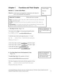
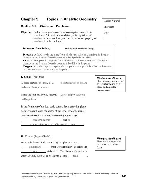
Chapter 9<br />
Section 9.1<br />
Topics in Analytic Geometry<br />
Circles and Parabolas<br />
Course Number<br />
Instructor<br />
Objective: In this lesson you learned how to recognize conics, write<br />
equations of circles in standard form, write equations of<br />
parabolas in standard form, and use the reflective property of<br />
parabolas to solve problems.<br />
Date<br />
Important Vocabulary<br />
Define each term or concept.<br />
Directrix A fixed line in the plane from which each point on a parabola is the same<br />
distance as the distance from the point to a fixed point in the plane.<br />
Focus A fixed point in the plane from which each point on a parabola is the same<br />
distance as the distance from the point to a fixed line in the plane.<br />
Tangent A line is tangent to a parabola at a point on the parabola if the line intersects,<br />
but does not cross, the parabola at the point.<br />
I. Conics (Page 660)<br />
A conic section, or conic, is . . .<br />
and a double-napped cone.<br />
Name the four basic conic sections:<br />
and hyperbola.<br />
the intersection of a plane<br />
circle, ellipse, parabola,<br />
What you should learn<br />
How to recognize a conic<br />
as the intersection of a<br />
plane and a doublenapped<br />
cone<br />
In the formation of the four basic conics, the intersecting plane<br />
does not pass through the vertex of the cone. When the plane<br />
does pass through the vertex, the resulting figure is a(n)<br />
degenerate conic , such as<br />
a point, a line, or a pair of intersecting lines<br />
.<br />
II. Circles (Pages 661−662)<br />
A circle is the set of all points (x, y) in a plane that are<br />
equidistant from a fixed point (h, k), called the<br />
center of the circle. The distance r between the<br />
center and any point (x, y) on the circle is the radius .<br />
What you should learn<br />
How to write equations<br />
of circles in standard<br />
form<br />
Larson/Hostetler/Edwards Precalculus with Limits: A Graphing Approach, Fifth Edition Student Notetaking Guide IAE<br />
Copyright © Houghton Mifflin Company. All rights reserved. 149
150 Chapter 9 Topics in Analytic Geometry<br />
The standard form of the equation of a circle with center<br />
(h, k) and radius r is (x − h) 2 + (y − k) 2 = r 2 .<br />
The standard form of the equation of a circle with radius r and<br />
whose center is the origin is x 2 + y 2 = r 2 .<br />
Example 1: The point (0, 1) is on a circle whose center is<br />
(−2, 1), as shown in the figure. Write the standard<br />
form of the equation of the circle.<br />
(x + 2) 2 + (y − 1) 2 = 4<br />
5<br />
y<br />
3<br />
1<br />
-5 -3 -1<br />
-1<br />
1 3 x<br />
5<br />
-3<br />
-5<br />
III. Parabolas (Pages 663−665)<br />
A parabola is . . . the set of all points (x, y) in a plane that<br />
are equidistant from a fixed line, the directrix, and a fixed point,<br />
the focus, not on the line.<br />
What you should learn<br />
How to write equations<br />
of parabolas in standard<br />
form<br />
The midpoint between the focus and the directrix is the<br />
vertex of a parabola. The line passing through the<br />
focus and the vertex is the axis of the parabola.<br />
The standard form of the equation of a parabola with a vertical<br />
axis having a vertex at (h, k) and directrix y = k − p is<br />
(x − h) 2 = 4p(y − k), p ≠ 0<br />
The standard form of the equation of a parabola with a horizontal<br />
axis having a vertex at (h, k) and directrix x = h − p is<br />
(y − k) 2 = 4p(x − h), p ≠ 0<br />
The focus lies on the axis p units (directed distance) from the<br />
vertex. If the vertex is at the origin (0, 0), the equation takes one<br />
of the following forms:<br />
x 2 = 4py, vertical axis or y 2 = 4px, horizontal axis<br />
Larson/Hostetler/Edwards Precalculus with Limits: A Graphing Approach, Fifth Edition Student Notetaking Guide IAE<br />
Copyright © Houghton Mifflin Company. All rights reserved.
Section 9.1 Circles and Parabolas 151<br />
Example 2: Find the standard form of the equation of the<br />
parabola with vertex at the origin and focus (1, 0).<br />
y 2 = 4x<br />
IV. Reflective Property of Parabolas (Pages 665−666)<br />
Describe a real-life situation in which parabolas are used.<br />
Answers will vary.<br />
What you should learn<br />
How to use the reflective<br />
property of parabolas to<br />
solve real-life problems<br />
A focal chord is . . . a line segment that passes through the<br />
focus of a parabola and has endpoints on the parabola.<br />
The specific focal chord perpendicular to the axis of a parabola<br />
is called the latus rectum .<br />
The reflective property of a parabola states that the tangent line<br />
to a parabola at a point P makes equal angles with the following<br />
two lines:<br />
1) The line passing through P and the focus<br />
2) The axis of the parabola<br />
y<br />
y<br />
y<br />
x<br />
x<br />
x<br />
Larson/Hostetler/Edwards Precalculus with Limits: A Graphing Approach, Fifth Edition Student Notetaking Guide IAE<br />
Copyright © Houghton Mifflin Company. All rights reserved.
152 Chapter 9 Topics in Analytic Geometry<br />
Additional <strong>notes</strong><br />
y<br />
y<br />
y<br />
x<br />
x<br />
x<br />
y<br />
y<br />
y<br />
x<br />
x<br />
x<br />
Homework Assignment<br />
Page(s)<br />
Exercises<br />
Larson/Hostetler/Edwards Precalculus with Limits: A Graphing Approach, Fifth Edition Student Notetaking Guide IAE<br />
Copyright © Houghton Mifflin Company. All rights reserved.
Section 9.2 Ellipses 153<br />
Section 9.2<br />
Ellipses<br />
Objective: In this lesson you learned how to write the standard form of<br />
the equation of an ellipse, and analyze and sketch the graphs<br />
of ellipses.<br />
Course Number<br />
Instructor<br />
Date<br />
Important Vocabulary<br />
Define each term or concept.<br />
Foci Distinct fixed points in the plane such that the sum of the distances from each<br />
point on an ellipse is constant.<br />
Vertices Points of intersection of an ellipse and the line through its foci.<br />
Major axis The chord connecting the vertices of an ellipse.<br />
Center The midpoint of the major axis of an ellipse.<br />
Minor axis The chord perpendicular to the major axis at the center of an ellipse.<br />
I. Introduction (Pages 671−674)<br />
An ellipse is . . . the set of all points (x, y) in a plane, the<br />
sum of whose distances from two distinct fixed points (foci) is<br />
constant.<br />
What you should learn<br />
How to write equations<br />
of ellipses in standard<br />
form<br />
The standard form of the equation of an ellipse with center (h, k)<br />
and a horizontal major axis of length 2a and a minor axis of<br />
length 2b, where 0 < b < a, is: (x − h) 2 /a 2 + (y − k) 2 /b 2 = 1<br />
The standard form of the equation of an ellipse with center (h, k)<br />
and a vertical major axis of length 2a and a minor axis of length<br />
2b, where 0 < b < a, is: (x − h) 2 /b 2 + (y − k) 2 /a 2 = 1<br />
In both cases, the foci lie on the major axis, c units from the<br />
center, with c 2 = a 2 − b 2 .<br />
If the center is at the origin (0, 0), the equation takes one of the<br />
following forms: x 2 /a 2 + y 2 /b 2 = 1 or<br />
x 2 /b 2 + y 2 /a 2 = 1 .<br />
Larson/Hostetler/Edwards Precalculus with Limits: A Graphing Approach, Fifth Edition Student Notetaking Guide IAE<br />
Copyright © Houghton Mifflin Company. All rights reserved.
154 Chapter 9 Topics in Analytic Geometry<br />
Example 1: Sketch the ellipse given by 4x + 25y<br />
= 100 .<br />
5<br />
y<br />
2<br />
2<br />
3<br />
1<br />
x<br />
-5 -3 -1 1 3 5<br />
-1<br />
-3<br />
-5<br />
II. Applications of Ellipses (Page 675)<br />
Describe a real-life application in which parabolas are used.<br />
Answers will vary.<br />
What you should learn<br />
How to use properties of<br />
ellipses to model and<br />
solve real-life problems<br />
III. Eccentricity (Page 676)<br />
Eccentricity measures the ovalness of an ellipse. It is<br />
given by the ratio e = c/a . For every ellipse, the<br />
value of e lies between 0 and 1 . For an<br />
elongated ellipse, the value of e is close to 1 .<br />
What you should learn<br />
How to find eccentricities<br />
of ellipses<br />
y<br />
y<br />
y<br />
x<br />
x<br />
x<br />
Homework Assignment<br />
Page(s)<br />
Exercises<br />
Larson/Hostetler/Edwards Precalculus with Limits: A Graphing Approach, Fifth Edition Student Notetaking Guide IAE<br />
Copyright © Houghton Mifflin Company. All rights reserved.
Section 9.3 Hyperbolas 155<br />
Section 9.3<br />
Hyperbolas<br />
Objective: In this lesson you learned how to write the standard form of<br />
the equation of a hyperbola, and analyze and sketch the<br />
graphs of hyperbolas.<br />
Course Number<br />
Instructor<br />
Date<br />
Important Vocabulary<br />
Define each term or concept.<br />
Branches The two disconnected parts of the graph of a hyperbola.<br />
Transverse axis The line segment connecting the vertices of a hyperbola.<br />
Conjugate axis The line segment in a hyperbola of length 2b joining (h, k + b) and<br />
(h, k − b) [or (h − b, k) and (h + b, k)].<br />
I. Introduction (Pages 680−681)<br />
A hyperbola is . . . the set of all points (x, y) in a plane the<br />
difference of whose distances from two distinct points (foci) is a<br />
positive constant.<br />
What you should learn<br />
How to write equations<br />
of hyperbolas in standard<br />
form<br />
The line through a hyperbola’s two foci intersects the hyperbola<br />
at two points called vertices .<br />
The midpoint of a hyperbola’s transverse axis is the<br />
center of the hyperbola.<br />
The standard form of the equation of a hyperbola centered at<br />
(h, k) and having a horizontal transverse axis is<br />
(x − h) 2 /a 2 − (y − k) 2 /b 2 = 1<br />
The standard form of the equation of a hyperbola centered at<br />
(h, k) and having a vertical transverse axis is<br />
(y − k) 2 /a 2 − (x − h) 2 /b 2 = 1<br />
In each case, the vertices and foci are, respectively, a and c units<br />
from the center. Moreover, a, b, and c are related by the equation<br />
c 2 = a 2 + b 2 .<br />
If the center of the hyperbola is at the origin (0, 0), the equation<br />
takes one of the following forms: x 2 /a 2 − y 2 /b 2 = 1 or<br />
y 2 /a 2 − x 2 /b 2 = 1 .<br />
Larson/Hostetler/Edwards Precalculus with Limits: A Graphing Approach, Fifth Edition Student Notetaking Guide IAE<br />
Copyright © Houghton Mifflin Company. All rights reserved.
156 Chapter 9 Topics in Analytic Geometry<br />
II. Asymptotes of a Hyperbola (Pages 682−684)<br />
The asymptotes of a hyperbola with a horizontal transverse axis<br />
are y = k ± b/a (x − h) .<br />
The asymptotes of a hyperbola with a vertical transverse axis<br />
are y = k ± a/b (x − h) .<br />
What you should learn<br />
How to find asymptotes<br />
of and graph hyperbolas<br />
y<br />
Example 1: Sketch the graph of the hyperbola given by<br />
2 9 2 =<br />
y − x 9 .<br />
x<br />
The eccentricity of a hyperbola is e = c/a , where<br />
the values of e are greater than 1 .<br />
III. Applications of Hyperbolas (Page 685)<br />
Describe a real-life application in which hyperbolas occur or are<br />
used.<br />
Answers will vary.<br />
What you should learn<br />
How to use properties of<br />
hyperbolas to solve reallife<br />
problems<br />
IV. General Equations of Conics (Page 686)<br />
2 2<br />
The graph of Ax + Bxy + Cy + Dx + Ey + F = 0 is one of the<br />
following:<br />
1) Circle if A = C<br />
2) Parabola if AC = 0<br />
3) Ellipse if AC > 0<br />
4) Hyperbola if AC < 0<br />
What you should learn<br />
How to classify conics<br />
from their general<br />
equations<br />
Example 2: Classify the equation 9x<br />
+ y −18x<br />
− 4y<br />
+ 4 = 0<br />
as a circle, a parabola, an ellipse, or a hyperbola.<br />
Ellipse<br />
2<br />
2<br />
Homework Assignment<br />
Page(s)<br />
Exercises<br />
Larson/Hostetler/Edwards Precalculus with Limits: A Graphing Approach, Fifth Edition Student Notetaking Guide IAE<br />
Copyright © Houghton Mifflin Company. All rights reserved.
Section 9.4 Rotation and Systems of Quadratic Equations 157<br />
Section 9.4<br />
Rotation and Systems of Quadratic Equations<br />
Objective: In this lesson you learned how to eliminate the xy-term in<br />
equations of conics and classify conics.<br />
Course Number<br />
Instructor<br />
Date<br />
Important Vocabulary<br />
Define each term or concept.<br />
Discriminant The quantity B 2 − 4AC, of the general conic equation<br />
Ax 2 + Bxy + Cy 2 + Dx + Ey + F = 0, which can be used to classify the type of conic.<br />
I. Rotation (Pages 690−693)<br />
The general equation of a conic whose axes are rotated so that<br />
they are not parallel to either the x-axis or the y-axis contains<br />
a(n) xy-term .<br />
What you should learn<br />
How to rotate the<br />
coordinate axes to<br />
eliminate the xy-term in<br />
equations of conics<br />
To eliminate this term, you can use a procedure called rotation<br />
of axes , whose objective is to rotate the x- and y-axes<br />
until they are parallel to the axes of the conic.<br />
The general second-degree equation<br />
2<br />
2<br />
Ax + Bxy + Cy + Dx + Ey + F = 0 can be rewritten as<br />
2<br />
2<br />
A ′(<br />
x′<br />
) + C′<br />
( y′<br />
) + D′<br />
x′<br />
+ E′<br />
y′<br />
+ F ′ = 0 by rotating the<br />
coordinate axes through an angle θ, where<br />
cot 2θ = (A − C)/B .<br />
The coefficients of the new equation are obtained by making the<br />
substitutions x = x′ cos θ − y′ sin θ and<br />
y = x′ sin θ + y′ cos θ .<br />
II. Invariants Under Rotation (Pages 694−695)<br />
Invariant under rotation means . . . that a term or<br />
quantity in the equation of a conic remains the same during a<br />
rotation of the coordinate axes through an angle θ.<br />
What you should learn<br />
How to use the<br />
discriminant to classify<br />
conics<br />
Larson/Hostetler/Edwards Precalculus with Limits: A Graphing Approach, Fifth Edition Student Notetaking Guide IAE<br />
Copyright © Houghton Mifflin Company. All rights reserved.
158 Chapter 9 Topics in Analytic Geometry<br />
The rotation of the coordinate axes through an angle θ that<br />
2<br />
2<br />
transforms the equation Ax + Bxy + Cy + Dx + Ey + F = 0<br />
2<br />
2<br />
into the form A ′(<br />
x′<br />
) + C′<br />
( y′<br />
) + D′<br />
x′<br />
+ E′<br />
y′<br />
+ F ′ = 0 has the<br />
following rotation invariants:<br />
1) F = F ′<br />
2) A + C = A′ + C ′<br />
3) B 2 − 4AC = (B′) 2 − 4A′C ′<br />
2<br />
The graph of the equation Ax + Bxy + Cy + Dx + Ey + F = 0<br />
is, except in degenerate cases, determined by its discriminant as<br />
follows:<br />
1) Ellipse or circle if: B 2 − 4AC < 0<br />
2) Parabola if : B 2 − 4AC = 0<br />
3) Hyperbola if: B 2 − 4AC > 0<br />
2<br />
Example 1: Classify the graph of the following conic:<br />
2x<br />
2<br />
Parabola<br />
2<br />
+ 12xy<br />
+ 18y<br />
− 3y<br />
− 5 = 0<br />
III. Systems of Quadratic Equations (Page 696)<br />
To find the points of intersection of two conics, . . . use<br />
either the elimination method or the substitution method.<br />
What you should learn<br />
How to solve systems of<br />
quadratic equations<br />
Example 2: Solve the following system of quadratic equations:<br />
⎪⎧<br />
2 2<br />
4x<br />
+ 4y<br />
− 36 = 0<br />
⎨<br />
2<br />
⎪⎩ x − 3y<br />
− 6x<br />
+ 9 = 0<br />
(0, 3) and (3, 0)<br />
Homework Assignment<br />
Page(s)<br />
Exercises<br />
Larson/Hostetler/Edwards Precalculus with Limits: A Graphing Approach, Fifth Edition Student Notetaking Guide IAE<br />
Copyright © Houghton Mifflin Company. All rights reserved.
Section 9.5 Parametric Equations 159<br />
Section 9.5<br />
Parametric Equations<br />
Objective: In this lesson you learned how to evaluate sets of parametric<br />
equations for given values of the parameter and graph curves<br />
that are represented by sets of parametric equations and how<br />
to rewrite sets of parametric equations as single rectangular<br />
equations and find sets of parametric equations for graphs.<br />
Course Number<br />
Instructor<br />
Date<br />
Important Vocabulary<br />
Define each term or concept.<br />
Parameter A third variable t introduced into equations involving x and y that relates<br />
the position of a point to time.<br />
I. Plane Curves (Page 699)<br />
If f and g are continuous functions of t on an interval I, the set of<br />
ordered pairs (f(t), g(t)) is a(n) plane curve C. The<br />
equations given by x = f (t)<br />
and y = g(t) are parametric<br />
What you should learn<br />
How to evaluate sets of<br />
parametric equations for<br />
given values of the<br />
parameter<br />
equations for C, and t is the parameter .<br />
II. Sketching a Plane Curve (Pages 700−701)<br />
One way to sketch a curve represented by a pair of parametric<br />
equations is to plot points in the xy-plane . Each set<br />
of coordinates (x, y) is determined from a value chosen for the<br />
parameter t . By plotting the resulting points in the<br />
order of increasing values of t, you trace the curve in a specific<br />
direction, called the orientation of the curve.<br />
What you should learn<br />
How to graph curves that<br />
are represented by sets of<br />
parametric equations<br />
Example 1: Sketch the curve described by the parametric<br />
2 +<br />
equations x = t − 3 and y = t 1, −1≤<br />
t ≤ 3 .<br />
10<br />
y<br />
6<br />
2<br />
x<br />
-5 -3 -1 1 3 5<br />
-2<br />
-6<br />
-10<br />
Larson/Hostetler/Edwards Precalculus with Limits: A Graphing Approach, Fifth Edition Student Notetaking Guide IAE<br />
Copyright © Houghton Mifflin Company. All rights reserved.
160 Chapter 9 Topics in Analytic Geometry<br />
Another way to display a curve represented by a pair of<br />
parametric equations is to use a graphing utility. To do so, . . .<br />
begin by setting the graphing utility to parametric mode, and<br />
enter the set of parametric equations as X 1T and Y 1T . When<br />
choosing a viewing window, you must set not only minimum<br />
and maximum values of x and y but also minimum and<br />
maximum values of t, the parameter.<br />
III. Eliminating the Parameter (Pages 702−703)<br />
Eliminating the parameter is the process of . . . finding a<br />
rectangular equation (in x and y) that has the same graph as a set<br />
of parametric equations.<br />
What you should learn<br />
How to rewrite sets of<br />
parametric equations as<br />
single rectangular<br />
equations by eliminating<br />
the parameter<br />
Describe the process used to eliminate the parameter from a set<br />
of parametric equations.<br />
Start with the set of parametric equations. Solve for t in one<br />
equation. Then substitute for t in the second parametric equation.<br />
Simplify. The resulting equation is a rectangular equation.<br />
When converting equations from parametric to rectangular form,<br />
it may be necessary to alter . . . the domain of the<br />
rectangular equation so that its graph matches the graph of the<br />
parametric equations.<br />
To eliminate the parameter in equations involving trigonometric<br />
functions, try using the identities . . .<br />
sin 2 θ + cos 2 θ = 1 or sec 2 θ − tan 2 θ = 1<br />
IV. Finding Parametric Equations for a Graph<br />
(Page 703)<br />
Describe how to find a set of parametric equations for a given<br />
graph.<br />
What you should learn<br />
How to find sets of<br />
parametric equations for<br />
graphs<br />
Answers will vary.<br />
Homework Assignment<br />
Page(s)<br />
Exercises<br />
Larson/Hostetler/Edwards Precalculus with Limits: A Graphing Approach, Fifth Edition Student Notetaking Guide IAE<br />
Copyright © Houghton Mifflin Company. All rights reserved.
Section 9.6 Polar Coordinates 161<br />
Section 9.6<br />
Polar Coordinates<br />
Objective: In this lesson you learned how to plot points in the polar<br />
coordinate system and convert equations from rectangular to<br />
polar form and vice versa.<br />
Course Number<br />
Instructor<br />
Date<br />
I. Introduction (Pages 707−708)<br />
To form the polar coordinate system in the plane, fix a point O,<br />
called the pole or origin , and construct<br />
from O an initial ray called the polar axis . Then each<br />
point P in the plane can be assigned polar coordinates (r, θ)<br />
as follows:<br />
What you should learn<br />
How to plot points and<br />
find multiple<br />
representations of points<br />
in the polar coordinate<br />
system<br />
1) r = directed distance from O to P<br />
2) θ = directed angle, counterclockwise from polar axis to<br />
the segment from O to P<br />
In the polar coordinate system, points do not have a unique<br />
representation. For instance, the point (r, θ) can be represented<br />
as (r, θ ± 2nπ) or (− r, θ ± (2n + 1)π) ,<br />
where n is any integer. Moreover, the pole is represented by<br />
(0, θ), where θ is any angle .<br />
Example 1: Plot the point (r, θ) = (− 2, 11π/4) on the polar<br />
coordinate system.<br />
π/2 y<br />
π<br />
x0<br />
3π/2<br />
Example 2: Find another polar representation of the point<br />
(4, π/6).<br />
Answers will vary. One such point is (− 4, 7π/6).<br />
Larson/Hostetler/Edwards Precalculus with Limits: A Graphing Approach, Fifth Edition Student Notetaking Guide IAE<br />
Copyright © Houghton Mifflin Company. All rights reserved.
162 Chapter 9 Topics in Analytic Geometry<br />
II. Coordinate Conversion (Pages 708−709)<br />
The polar coordinates (r, θ) are related to the rectangular<br />
coordinates (x, y) as follows . . .<br />
What you should learn<br />
How to convert points<br />
from rectangular to polar<br />
form and vice versa<br />
x = r cos θ<br />
y = r sin θ<br />
tan θ = y/x r 2 = x 2 + y 2<br />
Example 3: Convert the polar coordinates (3, 3π/2) to<br />
rectangular coordinates.<br />
(0, − 3)<br />
III. Equation Conversion (Page 710)<br />
To convert a rectangular equation to polar form, . . .<br />
simply replace x by r cos θ and y by r sin θ, and simplify.<br />
What you should learn<br />
How to convert equations<br />
from rectangular to polar<br />
form and vice versa<br />
Example 4: Find the rectangular equation corresponding to the<br />
− 5<br />
polar equation r = .<br />
sinθ<br />
y = − 5<br />
π/2 y<br />
π/2 y<br />
π/2 y<br />
π<br />
x0<br />
π<br />
x0<br />
π<br />
x0<br />
3π/2<br />
Homework Assignment<br />
Page(s)<br />
Exercises<br />
3π/2<br />
3π/2<br />
Larson/Hostetler/Edwards Precalculus with Limits: A Graphing Approach, Fifth Edition Student Notetaking Guide IAE<br />
Copyright © Houghton Mifflin Company. All rights reserved.
Section 9.7 Graphs of Polar Equations 163<br />
Section 9.7 Graphs of Polar Equations<br />
Objective: In this lesson you learned how to graph polar equations.<br />
I. Introduction (Pages 713−714)<br />
Example 1: Use point plotting to sketch the graph of the polar<br />
equation r = 3cosθ<br />
.<br />
π/2 y<br />
Course Number<br />
Instructor<br />
Date<br />
What you should learn<br />
How to graph polar<br />
equations by point<br />
plotting<br />
π<br />
x0<br />
3π/2<br />
The graph of the polar equation r = f (θ ) can be rewritten in<br />
parametric form, using t as a parameter, as follows:<br />
x = f(t) cos t and y = f(t) sin t<br />
II. Symmetry (Pages 714−715)<br />
The graph of a polar equation is symmetric with respect to the<br />
following if the given substitution yields an equivalent equation.<br />
Substitution<br />
1) The line θ = π/2: Replace (r, θ) by (r, π − θ) or (− r, − θ)<br />
What you should learn<br />
How to use symmetry as<br />
a sketching aid<br />
2) The polar axis: Replace (r, θ) by (r, − θ) or (− r, π − θ)<br />
3) The pole: Replace (r, θ) by (r, π + θ) or (− r, θ)<br />
Example 2: Describe the symmetry of the polar equation<br />
r = 2(1<br />
− sinθ<br />
) .<br />
Symmetric with respect to the line θ = π/2<br />
III. Zeros and Maximum r-Values (Pages 716−717)<br />
Two additional aids to sketching graphs of polar equations are . . .<br />
knowing the θ-values for which | r | is maximum and knowing<br />
the θ-values for which r = 0.<br />
What you should learn<br />
How to use zeros and<br />
maximum r-values as<br />
sketching aids<br />
Larson/Hostetler/Edwards Precalculus with Limits: A Graphing Approach, Fifth Edition Student Notetaking Guide IAE<br />
Copyright © Houghton Mifflin Company. All rights reserved.
164 Chapter 9 Topics in Analytic Geometry<br />
Example 3: Describe the zeros and maximum r-values of the<br />
polar equation r = 5cos 2θ<br />
The maximum value of | r | is | r | = 5 when θ = 0,<br />
π/2, π, 3π/2; the zeros of r occur at θ = π/4, 3π/4,<br />
5π/4, 7π/4<br />
IV. Special Polar Graphs (Pages 718−719)<br />
List the general equations that yield each of the following types<br />
of special polar graphs:<br />
What you should learn<br />
How to recognize special<br />
polar graphs<br />
Limaçons: r = a ± b cos θ, r = a ± b sin θ, a > 0, b > 0<br />
Rose curves:<br />
r = a cos nθ, r = a sin nθ, n ≥ 2; n petals if n is odd; 2n petals if n is even<br />
Circles:<br />
r = a cos θ, r = a sin θ<br />
Lemniscates:<br />
r 2 = a 2 sin 2θ; r 2 = a 2 cos 2θ<br />
π/2 y<br />
π/2 y<br />
π/2 y<br />
π<br />
x0<br />
π<br />
x0<br />
π<br />
x0<br />
3π/2<br />
π/2 y<br />
3π/2<br />
π/2 y<br />
3π/2<br />
π/2 y<br />
π<br />
x0<br />
π<br />
x0<br />
π<br />
x0<br />
3π/2<br />
Homework Assignment<br />
Page(s)<br />
Exercises<br />
3π/2<br />
3π/2<br />
Larson/Hostetler/Edwards Precalculus with Limits: A Graphing Approach, Fifth Edition Student Notetaking Guide IAE<br />
Copyright © Houghton Mifflin Company. All rights reserved.
Section 9.8 Polar Equations of Conics 165<br />
Section 9.8 Polar Equations of Conics<br />
Objective: In this lesson you learned how to write conics in terms of<br />
eccentricity and to write equations of conics in polar form.<br />
Course Number<br />
Instructor<br />
Date<br />
I. Alternative Definition of Conics (Page 722)<br />
The locus of a point in the plane that moves so that its distance<br />
from a fixed point (focus) is in a constant ratio to its distance<br />
from a fixed line (directrix) is a conic . The constant<br />
ratio is the eccentricity of the conic and is<br />
denoted by e. Moreover, the conic is an ellipse if e < 1 ,<br />
a parabola if e = 1 , and a hyperbola if e > 1 .<br />
What you should learn<br />
How to define conics in<br />
terms of eccentricities<br />
For each type of conic, the focus is at the pole .<br />
II. Polar Equations of Conics (Pages 722−724)<br />
The graph of the polar equation r = ep/(1 + e cos θ)<br />
is a conic with a vertical directrix to the right of the pole, where<br />
e > 0 is the eccentricity and | p | is the distance between the focus<br />
(pole) and the directrix.<br />
What you should learn<br />
How to write and graph<br />
equations of conics in<br />
polar form<br />
The graph of the polar equation r = ep/(1 − e cos θ)<br />
is a conic with a vertical directrix to the left of the pole, where<br />
e > 0 is the eccentricity and | p | is the distance between the focus<br />
(pole) and the directrix.<br />
The graph of the polar equation r = ep/(1 + e sin θ)<br />
is a conic with a horizontal directrix above the pole, where e > 0<br />
is the eccentricity and | p | is the distance between the focus<br />
(pole) and the directrix.<br />
The graph of the polar equation r = ep/(1 − e sin θ)<br />
is a conic with a horizontal directrix below the pole, where e > 0<br />
Larson/Hostetler/Edwards Precalculus with Limits: A Graphing Approach, Fifth Edition Student Notetaking Guide IAE<br />
Copyright © Houghton Mifflin Company. All rights reserved.
166 Chapter 9 Topics in Analytic Geometry<br />
is the eccentricity and | p | is the distance between the focus<br />
(pole) and the directrix.<br />
Example 1: Identify the type of conic from the polar equation<br />
36<br />
r =<br />
, and describe its orientation.<br />
10 + 12sinθ<br />
Hyperbola with a horizontal directrix above the<br />
pole<br />
III. Applications (Page 725)<br />
Describe a real-life application of polar equations of conics.<br />
Answers will vary.<br />
What you should learn<br />
How to use equations of<br />
conics in polar form to<br />
model real-life problems<br />
π/2 y<br />
π/2 y<br />
π/2 y<br />
π<br />
x0<br />
π<br />
x0<br />
π<br />
x0<br />
3π/2<br />
π/2 y<br />
3π/2<br />
π/2 y<br />
3π/2<br />
π/2 y<br />
π<br />
x0<br />
π<br />
x0<br />
π<br />
x0<br />
3π/2<br />
Homework Assignment<br />
Page(s)<br />
Exercises<br />
3π/2<br />
3π/2<br />
Larson/Hostetler/Edwards Precalculus with Limits: A Graphing Approach, Fifth Edition Student Notetaking Guide IAE<br />
Copyright © Houghton Mifflin Company. All rights reserved.