Report

ESTIMATION OF POTENTIAL TRADE UNDER SAFTA WITH THE GRAVITY MODEL 45
gravity model developed in this paper is estimated by
using panel data approach with country-pair specific
as well as year-specific fixed effects.
We estimate Fixed Effect Model (FEM) and
Random Effect Model (REM). According to the
literature (Egger 2000) FEM is better suited to when
estimating typical trade flows between ex-ante
predetermined selections of countries. We also use
Hausman Test to arrive at the more appropriate model.
The test is undertaken for the null hypothesis of no
correlation between the individual effects and the
regressors. The test also indicates FEM to be more
appropriate. Likewise results of FEM are reported.
Since the effect of variables that do not change
overtime, e.g. distance cannot be estimated directly by
FEM as inherent transformation drops the variable,
we use two step method, i.e. we estimate in second step
using individual effects as dependent variable and
distance and other dummies as explanatory variables.
THE EMPIRICAL RESULTS FROM
THE GRAVITY MODEL
This section examines whether the factors indicated in
the gravity equation make a significant contribution
to an explanation of the trade flows in the SAFTA
region. The gravity model has been tested both for the
aggregate bilateral trade and also for product level
trade. In the literature, aggregate gravity model has been
estimated using different data set by Wang and Winters
(1991), Hamilton and Winters (1992), Baldwin (1994),
Breuss and Egger (1999), etc. Bergstand (1989) and
Feenstra et al. (2001) has estimated product specific
models. In the present study, it was not possible to
estimate gravity model for all sectors due to nonavailability
of sectoral data for the period under
consideration. Therefore, the gravity equation is fitted
on aggregate data and on some selected sectors. The
results for gravity equation are presented in the Table
5.1.
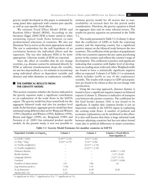
The results presented in Table 5.1 (Column 1) show
that the coefficient of GDPs in both the exporting
country and the importing country has a significant
positive impact on the bilateral trade between the two
countries. The coefficient of the product of populations
of the two countries captures the per capita purchasing
power in the country and reflects the country’s stage of
development. The coefficient is positive and significant
indicating that countries with higher level of development
are trading more with each other. Weighted tariffs
are found to have a statistically significant negative
effect as expected. Column 2 of Table 5.1 is estimated,
which includes tariffs as one of the explanatory
variable. The results with respect to GDP and population
are found to be robust as they do not change with
specification.
Using the two-step approach, distance dummy is
found to have a significant negative impact on bilateral
exports (Column 3). Distance is indicative of transport
cost between the partner countries. The coefficient for
the land border dummy (D4) is not found to be
significant. It implies that common border is not an
important variable in the SAFTA region in explaining
the existing trade flows. A number of political and
economic explanations can be attributed to this effect.
It is also well known that there is huge informal trade
between adjoining countries but has not taken formal
route due to political differences in major economies.
Table 5.1 Gravity Model Estimates for member countries in SAFTA
Dependent Variable: Ln Exports ijt
Column 1 Column 2 Column 3 (Fixed Effects
from Equation 2)
Ln (GDP i
* GDP j
) 0.44*** (3.45) 0.41** (2.82)
Ln (Pop i
* Pop j
) 0.34** (2.79) 0.34** (2.06)
Ln (Tariffs weighted) ji – –0.22** (–2.18)
Ln (Tariffs weighted) ij – –0.22** (–2.18)
Distance dummy – – –0.001* (–1.89)
Border dummy – – –1.37 (–0.64)
Language dummy – – 3.22** (2.22)
Constant – – 13.29*** (4.90)
Number of observations 231 198 42
Log Amemiya prob cr –1.96 1.97
R–sq (between) 0.71 0.59 0.20
Akaike Info. Crt. 1.25 1.36
* is significant at 10%; ** significant at 5%; *** significant at 1%.