Lecture 2: Descriptive Statistics and Exploratory Data Analysis

Lecture 2: Descriptive
Statistics and Exploratory
Data Analysis

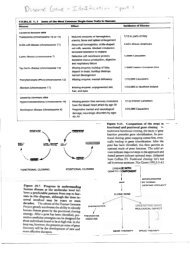
Further Thoughts on Experimental Design
• 16 Individuals (8 each from two populations) with replicates
Pop 1 Pop 2
Randomly sample 4 individuals from each pop
Tissue culture and RNA extraction
Labeling and array hybridization
Slide scanning and data acquisition
Repeat 2 times processing 16 samples in total
Repeat entire process producing 2 technical
replicates for all 16 samples

Other Business
• Course web-site:
http://www.gs.washington.edu/academics/courses/akey/56008/index.htm
• Homework due on Thursday not Tuesday
• Make sure you look at HW1 soon and see
either Shameek or myself with questions

Today
• What is descriptive statistics and exploratory
data analysis?
• Basic numerical summaries of data
• Basic graphical summaries of data
•How to use R for calculating descriptive statistics
and making graphs

“Central Dogma” of Statistics
Population
Probability
Descriptive
Statistics
Sample
Inferential Statistics

EDA
Before making inferences from data it is essential to
examine all your variables.
Why?
To listen to the data:
- to catch mistakes
- to see patterns in the data
- to find violations of statistical assumptions
- to generate hypotheses
…and because if you don’t, you will have trouble later

Types of Data
Categorical
Quantitative
binary
nominal
ordinal
discrete
continuous
2 categories
more categories
order matters
numerical
uninterrupted

Dimensionality of Data Sets
• Univariate: Measurement made on one variable per
subject
• Bivariate:
Measurement made on two variables per
subject
• Multivariate: Measurement made on many variables
per subject

Numerical Summaries of Data
• Central Tendency measures. They are computed
to give a “center” around which the measurements in
the data are distributed.
• Variation or Variability measures. They describe
“data spread” or how far away the measurements are
from the center.
• Relative Standing measures. They describe the
relative position of specific measurements in the data.

Location: Mean
1. The Mean
x
To calculate the average of a set of observations, add their
value and divide by the number of observations:
x = x 1
+ x 2
+ x 3
+ ...+ x n
n
= 1 n
n
" x i
i=1
!

Other Types of Means
Weighted means:
x =
n
"
i=1
n
"
i=1
w i
x i
w i
Trimmed:
x = "
!
Geometric:
#
x = %
$
n
"
i=1
x i
&
(
'
1
n
!
Harmonic:
x = n n
1
"
i=1
x i
!
!

Location: Median
• Median – the exact middle value
• Calculation:
- If there are an odd number of observations, find the middle value
- If there are an even number of observations, find the middle two
values and average them
• Example
Some data:
Age of participants: 17 19 21 22 23 23 23 38
Median = (22+23)/2 = 22.5

Which Location Measure Is Best?
• Mean is best for symmetric distributions without outliers
• Median is useful for skewed distributions or data with
outliers
0 1 2 3 4 5 6 7 8 9 10
0 1 2 3 4 5 6 7 8 9 10
Mean = 3
Mean = 4
Median = 3 Median = 3

Scale: Variance
• Average of squared deviations of values from
the mean
" ˆ
2 =
n
$
i
(x i
# x ) 2
n #1
!

Why Squared Deviations?
• Adding deviations will yield a sum of ?
• Absolute values do not have nice mathematical
properties
• Squares eliminate the negatives
• Result:
– Increasing contribution to the variance as you go
farther from the mean.

Scale: Standard Deviation
• Variance is somewhat arbitrary
• What does it mean to have a variance of 10.8? Or
2.2? Or 1459.092? Or 0.000001?
• Nothing. But if you could “standardize” that value,
you could talk about any variance (i.e. deviation) in
equivalent terms
• Standard deviations are simply the square root of the
variance

Scale: Standard Deviation
ˆ " =
n
$
i
(x i
# x ) 2
n #1
1. Score (in the units that are meaningful)
2. Mean
!
3. Each score’s s deviation from the mean
4. Square that deviation
5. Sum all the squared deviations (Sum of Squares)
6. Divide by n-1
7. Square root – now the value is in the units we started with!!!

Interesting Theoretical Result
• Regardless of how the data are distributed, a certain
percentage of values must fall within k standard deviations
from the mean:
Note use of µ (mu) to
represent “mean”.
At least
Note use of σ (sigma) to
represent “standard deviation.”
within
(1 - 1/1 2 ) = 0% …….….. k=1 (μ ± 1σ)
(1 - 1/2 2 ) = 75% …........ k=2 (μ ± 2σ)
(1 - 1/3 2 ) = 89% ………....k=3 (μ ± 3σ)

Often We Can Do Better
For many lists of observations – especially if their histogram is bell-shaped
1. Roughly 68% of the observations in the list lie within 1 standard
deviation of the average
2. 95% of the observations lie within 2 standard deviations of the
average
Ave-2s.d.
Ave-s.d.
Average
Ave+s.d.
Ave+2s.d.
68%
95%

Scale: Quartiles and IQR
IQR
25% 25% 25% 25%
Q 1 Q 2 Q 3
• The first quartile, Q 1
, is the value for which 25% of the
observations are smaller and 75% are larger
• Q 2
is the same as the median (50% are smaller, 50% are
larger)
• Only 25% of the observations are greater than the third
quartile

Percentiles (aka Quantiles)
In general the n th percentile is a value such that n% of the
observations fall at or below or it
n%
Q 1 = 25 th percentile
Median = 50 th percentile
Q 2 = 75 th percentile

Graphical Summaries of Data
A (Good) Picture Is
Worth A 1,000 Words

Univariate Data: Histograms and
Bar Plots
• What’s the difference between a histogram and bar plot?
Bar plot
• Used for categorical variables to show frequency or proportion in
each category.
• Translate the data from frequency tables into a pictorial
representation…
Histogram
• Used to visualize distribution (shape, center, range, variation) of
continuous variables
• “Bin size” important

Effect of Bin Size on Histogram
• Simulated 1000 N(0,1) and 500 N(1,1)
Frequency
Frequency
Frequency

More on Histograms
• What’s the difference between a frequency histogram
and a density histogram?

More on Histograms
• What’s the difference between a frequency histogram
and a density histogram?
Frequency Histogram
Density Histogram

100.0
66.7
Box Plots
Q 3
maximum
Years
33.3
IQR
Q 1
median
minimum
0.0
AGE
Variables

Bivariate Data
Variable 1 Variable 2 Display
Categorical Categorical Crosstabs
Stacked Box Plot
Categorical Continuous Boxplot
Continuous Continuous Scatterplot
Stacked Box Plot

Clustering
Multivariate Data
• Organize units into clusters
• Descriptive, not inferential
• Many approaches
• “Clusters” always produced
Data Reduction Approaches (PCA)
• Reduce n-dimensional dataset into much smaller number
• Finds a new (smaller) set of variables that retains most of
the information in the total sample
• Effective way to visualize multivariate data

How to Make a Bad Graph
The aim of good data graphics:
Display data accurately and clearly
Some rules for displaying data badly:
– Display as little information as possible
– Obscure what you do show (with chart junk)
– Use pseudo-3d and color gratuitously
– Make a pie chart (preferably in color and 3d)
– Use a poorly chosen scale
From Karl Broman: http://www.biostat.wisc.edu/~kbroman/

Example 1

Example 2

Example 3

Example 4

Example 5

R Tutorial
• Calculating descriptive statistics in R
• Useful R commands for working with multivariate
data (apply and its derivatives)
• Creating graphs for different types of data
(histograms, boxplots, scatterplots)
• Basic clustering and PCA analysis