Structure Preserving CAD Model Repair - OpenFlipper

More documents

Recommendations

Info

Stephan Bischoff & Leif Kobbelt / Structure Preserving CAD Model Repair Figure 1: Our algorithm converts a tessellated CAD model into an intersection-free and closed triangle mesh which covers all gaps up to a prescribed size. Left: The input patches were created by tessellating a CAD model consisting of 385 trimmed NURBS surfaces. Middle: A standard volumetric reconstruction algorithm resamples the model globally and destroys any structure of the tessellation. Right: Our algorithm only resamples the model locally in regions around artifacts like gaps and intersections and thus preserves most of the input tessellation. regions that are away from these inconsistencies. We are thus able to preserve any characteristic structure (e.g. isoparameter or curvature lines) that might be present in the input tessellation. Our algorithm closes gaps up to a userdefined maximum diameter, resolves intersections and overlaps, handles incompatible patch orientations and produces a feature-sensitive, manifold output that stays within a prescribed error-tolerance to the input model. The basic idea is to first identify the critical regions containing artifacts like gaps and overlaps, then selectively applying a volumetric reconstruction algorithm in these regions and finally joining the reconstruction with the unmodified outside components. Due to its selectivity our algorithm is on the one hand able to achieve high grid resolutions and thus a high reconstruction quality near the artifacts, but on the other hand does not incur the performance overhead of algorithms that globally reconstruct the input. 2. Previous Work Surface-based algorithms work directly on the input tessellation and use a number of techniques to detect and resolve artifacts. These techniques include, e.g. snapping boundary elements onto each other, projecting and inserting boundary edges into faces, explicitly computing the intersections between faces, propagating the normal field from patch to patch [BW92, BS95, BDK98, GTLH01, MD93], stitching small patches into gaps [TL94, Lie03], resolving topological noise by identifying and cutting handles [GW01], etc. Surface-based approaches only locally modify the input geometry in a small region around the artifacts. Hence, the input tessellation is preserved wherever possible. However, these approaches usually cannot give any guarantees on the quality of the output: There might be no globally consistent orientation of the input patches; certain artifacts, like overlapping geometry or “double walls” are hard to handle; intersections are difficult to detect and to resolve; due to numerical issues a robust and efficient implementation is challenging. Volume oriented approaches convert the input into a volumetric representation, i.e. a signed distance field or a grid of directed distances [NT03, Ju04, FPRJ00]. From this volumetric representation one then extracts a surface using techniques like marching cubes [LC87, KBSS01] or dual contouring [Gib98, JLSW02, Ju04]. Volumetric techniques produce guaranteed manifold output. Furthermore, topological artifacts and holes can easily be removed using various filter operations on the volume [ABA02,DMGL02,NT03]. On the downside, however, the conversion to and from a volume acts as a low-pass filter that removes sharp features and leads to aliasing artifacts in the reconstruction. Furthermore, due to the global resampling, the structure of the input patches is completely destroyed and the output is usually highly over-tessellated. 3. Algorithm The input to our algorithm is a tessellated CAD model M 0 = {P 1 ,...,P n} which consists of n patches P i . Each patch P i is a manifold triangle mesh and is uniquely identified by its patch ID i. Furthermore, the user prescribes an error tolerance ε 0 and a maximum gap diameter γ 0 . The output is an intersection-free and closed triangle mesh T that approximates M 0 up to a maximum error of ε 0 and covers all gaps of diameter ≤ γ 0 . Our algorithm proceeds in several stages (see Figure 2): c○ The Eurographics Association and Blackwell Publishing 2005.
Stephan Bischoff & Leif Kobbelt / Structure Preserving CAD Model Repair 1. Conversion of M 0 to a closed mesh M (Section 3.1) 2. Identification of a set C ⊂ Z 3 of critical vertices that encloses all intersections and all gaps of diameter ≤ γ 0 (Section 3.2) 3. Eroding C to a minimal set C ′ (Section 3.3) 4. Transforming C ′ to a set D of critical cells that covers all gaps and all intersections (Section 3.4) 5. Clipping M against D (Section 3.4) 6. Reconstruction of the model geometry inside D (Section 3.5) 7. 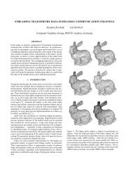Postprocessing to reduce the output complexity (Section 3.6) 1. input patches 2. critical vertices 3.1. Setup In the following we assume without loss of generality that the input model is scaled and translated such that the error tolerance ε 0 = 1 and that M 0 is enclosed by an integer grid of extent [0,2 k ] × [0,2 k ] × [0,2 k ] for some k. Note that the size of the grid cells just equals the error tolerance ε 0 . We also assume that the maximum gap diameter is given as γ 0 = 2γ for some positive integer γ. We often have to associate data with a small subset of the grid vertices or the grid cells. To improve memory efficiency, this data is stored in the finest-level nodes of an octree of depth k. The octree is adaptively refined on demand, i.e. when we access a certain grid vertex or grid cell. For each patch P i ∈ M 0 we produce a mirror patch P ′ i by duplicating P i and reversing the orientation of each triangle. Then we seam P i and P ′ i along their common boundary by triangle strips S i . This yields a new and closed patch Q i that represents P i from both sides. We collect the new patches in a new model M = {Q i }. Note that M is closed, but still contains the same artifacts as M 0 . Note also that by this construction our algorithm becomes invariant with respect to the orientation of the input patches. If it turns out that the resulting “double walls” are not necessary to guarantee manifoldness of the reconstruction, they will be removed in the post-processing stage, see Section 3.6. 3.2. Critical regions In the following we compute a set C γ of critical grid vertices. We think of these critical vertices as particles that fill those regions of space where two or more patches of M get closer than 2γ. These critical regions include all gaps of diameter ≤ 2γ and in particular all intersections between different patches. Later stages of the algorithm will then extract the interface between critical vertices and non-critical 3. critical cells 4. clipped 5. prelim. reconstruction 6. result Figure 2: Stages of our algorithm. The input patches typically exhibit artifacts like gaps and intersections (1). We determine a (rather large) set of critical vertices in a local neighborhood around these artifacts (2) and then convert these vertices into a (smaller) set of critical cells (3). The input patches are clipped against the critical cells (4) and the interior of the cells is reconstructed using a variant of the Marching Cubes algorithm (5). This preliminary reconstruction is then simplified to get the final result (6). Note that the model geometry away from the artifacts is not affected by our reconstruction algorithm and hence any structure in the input patches is well preserved. vertices to create surface patches that actually close the gaps and resolve the intersections. Let us call a grid vertex v ∈ Z 3 ambiguous if Box γ(v) := {w ∈ Z 3 : ||w − v|| ∞ ≤ γ} is intersected by two or more patches of M. If v is an ambiguous vertex, we set all vertices ∈ Box γ(v) to critical, i.e. C γ := [ v ambiguous Box γ(v) Figure 3 shows some configurations of M and the corresponding ambiguous and critical vertices. Ambiguous vertices can efficiently be located by using a (temporary) octree of depth k. We shift the origin of the octree by (.5,.5,.5) T such that the centers of the finest-level c○ The Eurographics Association and Blackwell Publishing 2005.
Page 1: EUROGRAPHICS 2005 / M. Alexa and J.
Page 5 and 6: Stephan Bischoff & Leif Kobbelt / S

Structure Preserving CAD Model Repair - OpenFlipper

You also want an ePaper? Increase the reach of your titles

Delete template?

Save as template?