Structure Preserving CAD Model Repair - OpenFlipper

EUROGRAPHICS 2005 / M. Alexa and J. Marks 

(Guest Editors) 

Volume 24 (2005), Number 3 

Structure Preserving CAD Model Repair 

Stephan Bischoff 

Leif Kobbelt 

Computer Graphics Group 

RWTH Aachen 

Abstract 

There are two major approaches for converting a tessellated CAD model that contains inconsistencies like cracks 

or intersections into a manifold and closed triangle mesh. Surface oriented algorithms try to fix the inconsistencies 

by perturbing the input only slightly, but they often cannot handle special cases. Volumetric algorithms on the other 

hand produce guaranteed manifold meshes but mostly destroy the structure of the input tessellation due to global 

resampling. In this paper we combine the advantages of both approaches: We exploit the topological simplicity 

of a voxel grid to reconstruct a cleaned up surface in the vicinity of intersections and cracks, but keep the input 

tessellation in regions that are away from these inconsistencies. We are thus able to preserve any characteristic 

structure (i.e. iso-parameter or curvature lines) that might be present in the input tessellation. Our algorithm closes 

gaps up to a user-defined maximum diameter, resolves intersections, handles incompatible patch orientations and 

produces a feature-sensitive, manifold output that stays within a prescribed error-tolerance to the input model. 

Categories and Subject Descriptors (according to ACM CCS): I.3.5 [Computational Geometry and Object Modeling]: 

Curve, surface, solid, and object representations 

1. Introduction 

A common dilemma in todays CAM production environments 

are the different geometry representations that are employed 

by CAD systems on the one hand and downstream 

applications on the other hand. While CAD systems usually 

represent a model by a set of trimmed NURBS patches or by 

other surface primitives (that possibly are extracted from a 

CSG representation), downstream applications like computational 

fluid- or structure simulation, rapid prototyping, and 

numerically controlled machining rely on closed and consistent 

manifold triangle meshes as input. The conversion from 

one representation into the other is not only a major bottleneck 

in terms of time, but also with respect to the accuracy 

and quality of the output and thus directly impacts all subsequent 

production stages. 

Common tessellation algorithms are able to efficiently 

and accurately convert single surface primitives into triangle 

meshes, but usually cannot handle continuity constraints between 

different primitives or detect and resolve intersecting 

geometry. This leads to artifacts like gaps, overlaps, intersections, 

or inconsistent orientations between the tessellated 

patches, which often have to be repaired in a manual and tedious 

postprocessing step. For this reason, quite some effort 

has been put into algorithms that are able to automatically 

repair such models. 

There are two major approaches for converting a tessellated 

CAD model that contains inconsistencies like gaps 

or intersections into a clean and manifold closed triangle 

mesh. Surface oriented algorithms try to explicitly compute 

or identify consistent (sub-)patches that are subsequently 

stitched together by snapping boundary elements. These algorithms 

only minimally perturb the input patches, but due 

to numerical issues cannot guarantee a consistent output 

mesh and hence usually require user-interaction. Volumetric 

algorithms on the other hand use a signed distance grid as 

an intermediate representation and are able to produce guaranteed 

manifold reconstructions. Unfortunately, these algorithms 

destroy the structure of the input tessellation due to 

a global resampling stage. Furthermore the resolution of the 

underlying grid limits the quality of the reconstruction. 

In this paper we combine the advantages of both approaches: 

We exploit the topological simplicity of a voxel 

grid to reconstruct a cleaned up surface in the vicinity of 

intersections and cracks, but keep the input tessellation in 

c○ The Eurographics Association and Blackwell Publishing 2005. Published by Blackwell 

Publishing, 9600 Garsington Road, Oxford OX4 2DQ, UK and 350 Main Street, Malden, 

MA 02148, USA.

Stephan Bischoff & Leif Kobbelt / Structure Preserving CAD Model Repair 

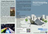
Figure 1: Our algorithm converts a tessellated CAD model into an intersection-free and closed triangle mesh which covers 

all gaps up to a prescribed size. Left: The input patches were created by tessellating a CAD model consisting of 385 trimmed 

NURBS surfaces. Middle: A standard volumetric reconstruction algorithm resamples the model globally and destroys any 

structure of the tessellation. Right: Our algorithm only resamples the model locally in regions around artifacts like gaps and 

intersections and thus preserves most of the input tessellation. 

regions that are away from these inconsistencies. We are 

thus able to preserve any characteristic structure (e.g. isoparameter 

or curvature lines) that might be present in the 

input tessellation. Our algorithm closes gaps up to a userdefined 

maximum diameter, resolves intersections and overlaps, 

handles incompatible patch orientations and produces 

a feature-sensitive, manifold output that stays within a prescribed 

error-tolerance to the input model. 

The basic idea is to first identify the critical regions containing 

artifacts like gaps and overlaps, then selectively applying 

a volumetric reconstruction algorithm in these regions 

and finally joining the reconstruction with the unmodified 

outside components. Due to its selectivity our algorithm 

is on the one hand able to achieve high grid resolutions and 

thus a high reconstruction quality near the artifacts, but on 

the other hand does not incur the performance overhead of 

algorithms that globally reconstruct the input. 

2. Previous Work 

Surface-based algorithms work directly on the input tessellation 

and use a number of techniques to detect and resolve 

artifacts. These techniques include, e.g. snapping boundary 

elements onto each other, projecting and inserting boundary 

edges into faces, explicitly computing the intersections 

between faces, propagating the normal field from patch to 

patch [BW92, BS95, BDK98, GTLH01, MD93], stitching 

small patches into gaps [TL94, Lie03], resolving topological 

noise by identifying and cutting handles [GW01], etc. 

Surface-based approaches only locally modify the input 

geometry in a small region around the artifacts. Hence, the 

input tessellation is preserved wherever possible. However, 

these approaches usually cannot give any guarantees on the 

quality of the output: There might be no globally consistent 

orientation of the input patches; certain artifacts, like overlapping 

geometry or “double walls” are hard to handle; intersections 

are difficult to detect and to resolve; due to numerical 

issues a robust and efficient implementation is challenging. 

Volume oriented approaches convert the input into a volumetric 

representation, i.e. a signed distance field or a grid 

of directed distances [NT03, Ju04, FPRJ00]. From this volumetric 

representation one then extracts a surface using techniques 

like marching cubes [LC87, KBSS01] or dual contouring 

[Gib98, JLSW02, Ju04]. 

Volumetric techniques produce guaranteed manifold output. 

Furthermore, topological artifacts and holes can easily 

be removed using various filter operations on the volume 

[ABA02,DMGL02,NT03]. On the downside, however, 

the conversion to and from a volume acts as a low-pass filter 

that removes sharp features and leads to aliasing artifacts 

in the reconstruction. Furthermore, due to the global resampling, 

the structure of the input patches is completely destroyed 

and the output is usually highly over-tessellated. 

3. Algorithm 

The input to our algorithm is a tessellated CAD model 

M 0 = {P 1 ,...,P n} which consists of n patches P i . Each 

patch P i is a manifold triangle mesh and is uniquely identified 

by its patch ID i. Furthermore, the user prescribes an 

error tolerance ε 0 and a maximum gap diameter γ 0 . The output 

is an intersection-free and closed triangle mesh T that 

approximates M 0 up to a maximum error of ε 0 and covers 

all gaps of diameter ≤ γ 0 . Our algorithm proceeds in several 

stages (see Figure 2): 

c○ The Eurographics Association and Blackwell Publishing 2005.


1. Conversion of M 0 to a closed mesh M (Section 3.1) 

2. Identification of a set C ⊂ Z 3 of critical vertices that 

encloses all intersections and all gaps of diameter ≤ γ 0 

(Section 3.2) 

3. Eroding C to a minimal set C ′ (Section 3.3) 

4. Transforming C ′ to a set D of critical cells that covers all 

gaps and all intersections (Section 3.4) 

5. Clipping M against D (Section 3.4) 

6. Reconstruction of the model geometry inside D (Section 

3.5) 

7. Postprocessing to reduce the output complexity (Section 

3.6) 

1. input patches 2. critical vertices 

3.1. Setup 

In the following we assume without loss of generality that 

the input model is scaled and translated such that the error 

tolerance ε 0 = 1 and that M 0 is enclosed by an integer grid 

of extent 

[0,2 k ] × [0,2 k ] × [0,2 k ] 

for some k. Note that the size of the grid cells just equals the 

error tolerance ε 0 . We also assume that the maximum gap 

diameter is given as γ 0 = 2γ for some positive integer γ. 

We often have to associate data with a small subset of 

the grid vertices or the grid cells. To improve memory efficiency, 

this data is stored in the finest-level nodes of an octree 

of depth k. The octree is adaptively refined on demand, 

i.e. when we access a certain grid vertex or grid cell. 

For each patch P i ∈ M 0 we produce 

a mirror patch P ′ i by duplicating P i and 

reversing the orientation of each triangle. 

Then we seam P i and P ′ i along their 

common boundary by triangle strips S i . 

This yields a new and closed patch Q i 

that represents P i from both sides. We 

collect the new patches in a new model 

M = {Q i }. Note that M is closed, but still contains the 

same artifacts as M 0 . Note also that by this construction our 

algorithm becomes invariant with respect to the orientation 

of the input patches. If it turns out that the resulting “double 

walls” are not necessary to guarantee manifoldness of the 

reconstruction, they will be removed in the post-processing 

stage, see Section 3.6. 

3.2. Critical regions 

In the following we compute a set C γ of critical grid vertices. 

We think of these critical vertices as particles that fill 

those regions of space where two or more patches of M get 

closer than 2γ. These critical regions include all gaps of diameter 

≤ 2γ and in particular all intersections between different 

patches. Later stages of the algorithm will then extract 

the interface between critical vertices and non-critical 

3. critical cells 4. clipped 

5. prelim. reconstruction 6. result 

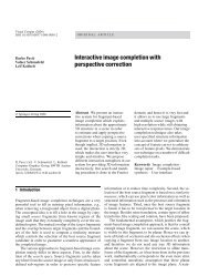
Figure 2: Stages of our algorithm. The input patches typically 

exhibit artifacts like gaps and intersections (1). We 

determine a (rather large) set of critical vertices in a local 

neighborhood around these artifacts (2) and then convert 

these vertices into a (smaller) set of critical cells (3). The input 

patches are clipped against the critical cells (4) and the 

interior of the cells is reconstructed using a variant of the 

Marching Cubes algorithm (5). This preliminary reconstruction 

is then simplified to get the final result (6). Note that the 

model geometry away from the artifacts is not affected by 

our reconstruction algorithm and hence any structure in the 

input patches is well preserved. 

vertices to create surface patches that actually close the gaps 

and resolve the intersections. 

Let us call a grid vertex v ∈ Z 3 ambiguous if 

Box γ(v) := {w ∈ Z 3 : ||w − v|| ∞ ≤ γ} 

is intersected by two or more patches of M. If v is an ambiguous 

vertex, we set all vertices ∈ Box γ(v) to critical, i.e. 

C γ := 

[ 

v ambiguous 

Box γ(v) 

Figure 3 shows some configurations of M and the corresponding 

ambiguous and critical vertices. 

Ambiguous vertices can efficiently be located by using 

a (temporary) octree of depth k. We shift the origin of the 

octree by (.5,.5,.5) T such that the centers of the finest-level 



octree nodes have integer coordinates, i.e. they correspond 

to grid vertices. If n is an octree node, we denote by c n ∈ Z 3 

its center and by 0 ≤ d n ≤ k its depth. Hence, if n is a finestlevel 

node (d n = k) we want to check whether 

Box(n) := Box γ(c n) 

is intersected by two or more different patches. Our idea is to 

build up a hierarchy of nested boxes which matches the octree 

hierarchy. Hence, if n is an interior octree node, Box(n) 

is chosen such that it contains the boxes of all descendants 

of n. A short calculation shows that this property is fulfilled 

by letting 

Box(n) := Box hn (c n), 

h n = 2 k−dn−1 − 1/2 + γ 

Note in particular, that a triangle intersecting the box of a 

finest-level node n will also intersect the boxes of all ancestors 

of n. We now recursively insert each triangle of M into 

the octree using an algorithm similar to that of Ju [Ju04]. 

Starting with the root node, a triangle is inserted into a node 

n if it intersects Box(n). This can efficiently be tested using 

the separating axes theorem [GLM96]. If a node n contains 

triangles belonging to different patches, n is split and the triangles 

are distributed to its children. In the end, the center 

c n ∈ Z 3 of each finest-level node n that contains triangles 

belonging to two or more patches represents an ambiguous 

vertex. 

To increase the resolution of the critical region near M, 

we also compute the directed distances of each critical vertex 

v ∈ C γ to M by shooting rays along the coordinate axes (Figure 

3). Fortunately, the temporary octree we built up above 

already provides a spatial search structure to speed up the 

ray-model intersection tests. If we find an intersection within 

unit distance, we denote the triple (v,d,δ) consisting of the 

vertex v, the direction 

d ∈ ±{(1,0,0) T ,(0,1,0) T ,(0,0,1) T } 

and the distance δ ∈ [0,1] as a cut. The cuts will later be 

used for resampling the geometry at the points v + δd. In 

the figures, cuts are illustrated as small arrows attached to v 

and pointing in direction d, see Figure 3. 

3.3. Eroding C γ 

In the previous stage we computed a set C := C γ of critical 

vertices which we think of as particles that fill in all gaps of 

M. Later stages of the algorithm will extract the boundary 

of C to create surface patches that actually close these gaps 

and resolve the intersections. As this fill-in should alter M 

as little as possible, C should be as small as possible. Hence 

we replace C by a minimal set C ′ ⊂ C that still fills in all 

gaps. We get C ′ by applying a topology-preserving erosion 

operator on C, i.e. we successively remove critical vertices 

from C that are simple. (Note that we only remove critical 

vertices but not the cuts.) Intuitively, a vertex is called simple, 

if its removal does not change the topology of C, i.e. if it 

patch ambiguous vertex 

cuts critical vertex ∈ C 1 

Figure 3: Example configurations. Some possible configurations 

of patches Q ∈ M are shown above. Note that each 

patch is a closed triangle mesh. The critical vertices C γ fill 

the regions where two or more different patches of M are 

less than 2γ away from each other. Cuts effectively provide 

sub-voxel accuracy near M. 

does not create new connected components or handles. The 

exact definition of simplicity and an efficient method to determine 

whether a vertex is simple from its 26-neighborhood 

is given in [BK03]. However, we have to take into account, 

that in our case the cuts represent material, while in [BK03] 

the cuts represent empty space. 

We proceed as follows: For each critical vertex v, we compute 

its distance d(v) to the boundary of C γ. If v has a noncritical 

neighbor, we set d(v) = 0. The distances of the other 

critical vertices are computed by a distance transform on C γ 

that respects the cuts, i.e. distances are not propagated over 

a cut. We then remove ⌈2γ⌉ layers of simple critical vertices 

to get a new set C ′ of critical vertices (Figures 4(left) and 5): 

for layer=0,1,...,⌈2γ⌉ do 

for all vertices v with d(v)=layer do 

if v is simple then 

set v to non-critical 

As the following reconstruction will take place along the 

cuts, there should be cuts between non-critical vertices w ∉ 

C ′ and critical vertices v ∈ C ′ . Furthermore, there should be 

no cuts between vertices v ∈ C ′ and M (Figures 4(right) 

and 5). Hence, if v is a critical vertex, we remove all cuts 

(v,d,δ) and instead insert cuts (w,v − w,δ smooth ) for all 



non-critical 6-neighbors w of v. Here, δ smooth is a special 

value to tell the reconstruction algorithm that w + δ smooth d 

corresponds to a fill-in and that the corresponding vertices 

should be smoothed in a postprocessing phase. 

Figure 4: Erosion. To the left we see the set C 2 of critical 

vertices that fills in a gap between two patches. The green 

vertices are removed by a topology-preserving erosion operation. 

The red vertices cannot be removed without disconnecting 

the two patches. Right: Each remaining (blue) vertex 

is replaced by cuts pointing into the vertex. All cuts now 

form the interface that is extracted in the later stages of the 

algorithm to close the gaps by surface patches. 

critical cell critical vertex ∈ C ′ 

removed cuts 

additional cuts 

Figure 5: Example configurations (cont.) The topologypreserving 

erosion operation (Section 3.3) shrinks C γ to a 

smaller set C ′ which is surrounded by additional cuts. Grid 

cells that are adjacent to a critical vertex ∈ C ′ or that are 

intersected by multiple patches are marked as critical (Section 

3.4). 

3.4. Clipping 

In this stage we clip M against a set of critical grid cells D 

into an inside and an outside component such that the inside 

component contains all the artifacts of the model. The inside 

component is then discarded and replaced by a well-behaved 

reconstruction as described in Section 3.5. 

First, we need to determine the set of critical grid cells D. 

As D should cover all artifacts of M, i.e. all intersections 

and all gaps, we set a grid cell to critical, 

• if it contains two or more patches of M (intersection) or 

• if one of its incident vertices is critical (gap) 

Figure 5 shows some example configurations of M and their 

corresponding critical grid cells. In the following, we will 

denote a grid face as critical, if it shares an un-critical and a 

critical cell. A grid edge is called critical, if it is incident to 

a critical face. 

The basic idea is to split all triangles of M along the critical 

faces into sub-triangles such that each sub-triangle either 

lies completely inside or completely outside the critical region 

D. We then simply discard those triangles that lie completely 

inside. 

Although the mathematics of intersecting planar faces is 

straightforward, the actual implementation of an efficient 

and numerically robust clipping algorithm is a hard problem. 

In the following we will present a new algorithm that is 

specifically tailored to our setup. 

• At all times during the run of the algorithm the meshes 

stay triangle meshes. We do not have to cope with general 

polygons of arbitrary valence, containing holes, etc. 

In fact, we modify the meshes using only the Euleroperations 

split-1-to-3 and split-2-to-4 (edge-split) which 

are provided as elementary operations by most mesh libraries. 

• By using a mixed fixed-point/adaptive-precision representation 

for the vertex locations, we achieve considerable 

speedups without sacrifying robustness or accuracy. 

The clipping proceeds in three phases which are illustrated 

in Figure 6. In phase I we intersect the critical edges 

and the model faces and insert the intersection points into 

the model using 1-to-3 or 2-to-4 splits. In phase II we intersect 

the critical faces and the model edges, again inserting 

the intersection points using 2-to-4 splits. This process automatically 

produces the edges that result from intersecting 

a model triangle with all critical grid faces. Thus each triangle 

now either lies completely inside or completely outside 

the critical cells. In phase III we then simply discard those 

triangles whose center of gravity lies in a critical cell. 

To effectively enumerate the critical edges and critical 

faces, we use the recursive octree traversal technique proposed 

by Ju et al [JLSW02]. However, to speed up the algorithm, 

before descending into an octree cell, we first test 



whether the current triangle really intersects the cell using 

the separating axis theorem. 

successful, we calculate the real intersection point using exact 

arithmetics. Analogous considerations apply for triangleedge 

intersections, edge-edge intersections, triangle-cell intersections, 

etc. 

Initial configuration 

Phase I 

3.5. Reconstruction 

We now present an algorithm to reconstruct the surface in 

the interior of the critical cells. This algorithm uses elements 

of the feature–sensitive marching cubes and dual contouring 

algorithms that were proposed by Kobbelt et al. [KBSS01] 

and Ju et al. [JLSW02] and later extended by Varadhan et 

al. [VKK ∗ 03] to arbitrary grids of directed distances. However, 

in addition to being feature-sensitive, our algorithm can 

also handle multiple cuts per edge and seamlessly connects 

the reconstruction inside the critical cells to the outside geometry. 

Phase II 

Phase III 

Figure 6: Initial configuration: A triangle mesh is to be 

clipped against a set of critical grid cells. Phase I: The intersections 

of the grid edges with the triangles are inserted 

into the mesh by 1-to-3-splits or 2-to-4-splits. Phase II: The 

intersections of mesh edges and grid faces are inserted by 

2-to-4-splits. Now each triangle either lies completely inside 

or completely outside the set of critical grid cells. Phase III: 

The interior triangles are discarded. 

Implementation The algorithm above only works if intersections 

are reliably detected and correctly calculated. However, 

just switching to exact arithmetics will extremely slow 

down the algorithm. For this reason, we use a mixed representation. 

Let the positions of the input vertices of the model 

be quantized to N bits. For each vertex v, we store 

• its exact position p exact,v using an adaptive precision representation 

[Pri91, She97]. 

• its approximate position p approx,v using a fixed point representation 

of N bits width 

such that (remember that the extent of the grid is 2 k ): 

||p exact,v − p approx,v|| < η := 2 k−N 

We can then use the approximate positions for evaluating 

“easy rejects” when computing intersection points. Consider 

for example the intersection of an edge e and a grid face 

f = [f min ,f max]. We first check whether e approx intersects the 

box 

[f min − (η,η,η) T ,f max + (η,η,η) T ] 

This test can exactly be evaluated in fixed-point arithmetics 

using a maximum of 3N bits only [Ju04]. Only if this test is 

We first enumerate all interior grid faces, again using a 

recursive octree traversal technique. For each interior grid 

face, we collect the cuts that are located on the edges of this 

face. Note that a grid edge might support more than two cuts, 

if a single patch intersects that edge multiple times. By construction, 

the number of cuts is always even. Furthermore, 

cuts pointing in clockwise (cw) direction alternate with cuts 

pointing in counter-clockwise (ccw) direction. We now connect 

these cuts by edges: a cw cut is connected to the next 

ccw cut by going ccw around the grid face (Figure 7, left), 

see also [Blo88, NH91]. If we connect two cuts from the 

same grid edge, we insert an auxiliary point at the face center 

to prevent topological degeneracies. Note that by construction, 

the edges do not intersect. 

We then visit each critical cell in turn. The edges on the 

cell’s faces were either created as described above or are 

boundary edges of the outside geometry. In any case, these 

edges form one or more connected loops around the cell. 

Each of these loops is triangulated by a triangle fan (Figure 

7, right). As the edges do not intersect, the loops will 

also be free of intersections and so are the triangle fans. 

Figure 7: We connect the cuts incident to a grid face by 

edges (left). For each grid cell these edges and the boundary 

edges of the outside geometry form loops around the 

cell. Each of these loops is triangulated by a fan of triangles 

(right). 



The position p of the fan’s center vertex is computed by 

minimizing the squared distances to the supporting planes of 

the triangles that intersect the grid cell [Lin00]. Note that, if 

the cell contains a feature edge or corner, this construction 

will place p exactly on the feature. If the computed point 

p happens to lie outside the cell or if it does not lie on all 

supporting planes, it is set to invalid. Invalid vertices are 

smoothed in the post-processing stage. Finally we flip the 

edges in interior grid faces, such that the center vertices become 

connected. This guarantees feature vertices in neighboring 

cells to be connected by a (feature) edge (Figure 8). 

In both cases we smooth the vertex positions by applying an 

iterative smoothing filter [Tau95]. 

Decimation The output of the reconstruction algorithm is 

a closed and manifold triangle mesh T which approximates 

the input model M but has all artifacts resolved. However, 

T usually contains much more vertices and faces than M 0 

due to the artificial refinement near the gaps. This can be 

attributed to two effects 

• Every patch of the input model is represented from both 

sides by T . 

• The higher the resolution of the underlying grid, the more 

triangles are needed for reconstructing the model in the 

critical regions. 

Accordingly, we have two options for reducing the output 

complexity. First, the mesh T usually consists of multiple 

connected components, only few of which really contribute 

to the outside of M. The other components merely triangulate 

M from the inside and hence can be easily identified 

and discarded. The identification can be done manually or 

automatically by a flood fill process as in [Ju04]. Second, 

we apply a standard feature-sensitive mesh decimation algorithm 

to T [GH97]. However, to preserve the input tessellation 

of M, we only do this in regions that were reconstructed 

anyway. 

4. Results 

sampled vertex 

smoothed vertex 

Figure 8: Example configurations (cont.) The geometry in 

the critical grid cells is replaced by a reconstructed surface 

R which is extracted from the cuts using a variant of the 

Marching Cubes algorithm. Some of the vertices of R can 

directly be sampled from M. Others, however, correspond 

to those parts of R that cover the gaps of M. The position of 

these vertices is determined by an iterative smoothing filter. 

3.6. Postprocessing 

Smoothing After the reconstruction stage the positions of 

the following types of vertices is not yet determined. 

• Vertices that correspond to those parts of the reconstruction 

that span gaps of M and hence have no canonical position. 

These are the vertices that either are derived from 

cuts (v,d,δ smooth ) or are the centers of triangle fans that 

are created in an empty grid cell. 

• Vertices that are the centers of triangle fans in grid cells 

that contain conflicting geometry — usually due to an insufficient 

refinement depth k. 

We have evaluated our method on a number of CAD models 

of different complexities (Figures 9, 10, 11). All timings 

were taken on a 2GB, 3.2 GHz Pentium 4 computer. 

Choice of input parameters As our algorithm only reconstructs 

the regions around artifacts and as this local reconstruction 

is further decimated in the postprocessing phase, 

the output complexity grows typically only sub-linearly with 

respect to the grid resolution. Hence we can use high grid 

resolutions to improve the reconstruction quality without incuring 

an undue overhead of generated triangles. If the tessellation 

of the input patches is sufficiently accurate, we can 

set γ = 1 without missing any gaps even for high resolutions. 

Asymptotic behaviour If the artifacts form a one dimensional 

subspace e.g. along the intersection of two surfaces 

or along two abutting patches, the number of critical vertices 

and cells should in theory grow linearly with respect to 

the grid resolution for a constant γ. Our experimental results 

match well with this theoretical statement, only the Camera 

model (Figure 10) is an exception because it contains a lot 

of interior geometry and “double walls”. These artifacts cannot 

suffiently be resolved and hence the critical vertices and 

cells actually form a two or three-dimensional subspace. In 

these regions the octree has to be refined to maximum depth, 

which causes a significant increase in memory usage. 



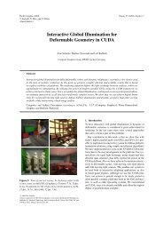
Helicopter, 10 k triangles in 60 patches, γ = 1 

resolution 1024 3 2048 3 4096 3 8192 3 

#critical vertices 242 k 505 k 1037 k 2079 k 

#critical cells 68 k 141 k 277 k 561 k 

#output triangles 28 k 34 k 44 k 60 k 

time 47 s 116 s 291 s 868 s 

Camera, 19 k triangles in 83 patches, γ = 1 

resolution 128 3 256 3 512 3 

#critical vertices 192 k 655 k 1978 k 

#critical cells 83 k 270 k 874 k 

#output triangles 33 k 61 k 81 k 

time 56 s 145 s 639 s 

Figure 10: Camera 

Figure 9: Helicopter 

5. Discussion 

We have presented a new and efficient algorithm for fully 

automatic and selective repair of tessellated CAD models. 

However, a number of issues are still open for future work. 

Artifacts within a single patch Our algorithm does reliably 

detect and resolve artifacts between different patches. 

However, it does not resolve artifacts within a single patch, 

like e.g. self-intersections. Of course, we could extend our 

algorithm to also handle such artifacts, but that would significantly 

decrease its performance. The reason is, that during 

the construction of the vertex octree, we often have to check 

whether a certain box contains two or more patches. Currently 

this check is very fast, as we only have to compare the 

patch IDs of the participating triangles. However, if we also 

wanted to detect self-intersections within a single patch, we 

would actually have to intersect each triangle with all other 

triangles in the box. This can be done very fast [SAUK04] 

but as none of our models has self-intersecting patches, we 

conclude that such a situation does not happen very often in 

practice. If it does, the user has to manually divide the patch 

into non-self-intersecting subpatches. 

Selectivity Our algorithm does only modify critical regions 

of the model, i.e. regions containing intersections or gaps, 

and preserves the structure of the tessellation everywhere 

else. These critical regions are determined fully automatically 

from a global user-defined parameter γ 0 . It should, 

however, be possible to let this parameter locally depend on 

the underlying model geometry such as to close gaps of different 

sizes. It should also be possible to apply one of the 

surface oriented mesh repair algorithms in a preprocessing 

step to segment the input into large and manifold patches 

wherever possible and apply our method only to those regions 

where the surface oriented methods fail. 

Reconstruction We reconstruct the surface in the critical 

regions from a grid of directed distances using a novel 

contouring algorithm. This algorithm correctly resolves any 

self-intersections based on the local configuration of the cuts 

around a grid face only. However, other (possibly global) 

criteria might also be incorporated. For example, we might 

strive for a reconstruction of minimal genus or of minimal 

number of connected components. For a standard grid of 

signed distances and the Marching Cubes algorithm, this has 

already been explored by Andujar et al. [ABC ∗ 04]. 

Space and time efficiency Due to its selectivity, our algorithm 

already proved to be quite space and time efficient. 

In our implementation we have used standard libraries for 

the octree and mesh data structures and for the exact arithmetic 

and the mesh decimation framework. We believe that 

we could achieve considerable speed ups and lower memory 

usage if we used custom-tailored data structures and algorithms 

instead. As our algorithm operates on local information 

only, it should also be easily possible to generalize it to 

parallel machines. 



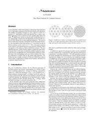
Ventilator, 269 k triangles in 12 patches, γ = 2 

resolution 1024 3 2048 3 4096 3 8192 3 

#critical vertices 238 k 460 k 828 k 1649 k 

#critical cells 64 k 113 k 229 k 523 k 

#output triangles 503 k 512 k 529 k 556 k 

time 83 s 123 s 193 s 303 s 

References 

Figure 11: Ventilator 

[ABA02] ANDUJAR C., BRUNET P., AYALA D.: 

Topology-reducing surface simplification using a discrete 

solid representation. ACM Trans. Graph. 21, 2 (2002), 

88–105. 

[ABC ∗ 04] ANDUJAR C., BRUNET P., CHICA A., 

NAVAZO I., ROSSIGNAC J., VINACUA A.: Optimizing 

the topological and combinatorial complexity of isosurfaces. 

Computer-Aided Design to appear (2004). 

[BDK98] BAREQUET G., DUNCAN C., KUMAR S.: 

RSVP: A geometric toolkit for controlled repair of solid 

models. IEEE Trans. on Visualization and Computer 

Graphics 4, 2 (1998), 162–177. 

[BK03] BISCHOFF S., KOBBELT L.: Sub-voxel topology 

control for level-set surfaces. Computer Graphics Forum 

22, 3 (September 2003), 273–280. 

[Blo88] BLOOMENTHAL J.: Polygonization of implicit 

surfaces. Computer Aided Geometric Design 5, 4 (1988), 

341–355. 

[BS95] BAREQUET G., SHARIR M.: Filling gaps in the 

boundary of a polyhedron. Computer-Aided Geometric 

Design 12, 2 (1995), 207–229. 

[BW92] BØHN J. H., WOZNY M. J.: Automatic CAD 

model repair: Shell-closure. In Proc. Symp. on Solid 

Freeform Fabrication (1992), pp. 86–94. 

[DMGL02] DAVIS J., MARSCHNER S., GARR M., 

LEVOY M.: Filling holes in complex surfaces using volumetric 

diffusion. In Proc. International Symposium on 

3D Data Processing, Visualization, Transmission (2002), 

pp. 428–438. 

[FPRJ00] FRISKEN S. F., PERRY R. N., ROCKWOOD 

A. P., JONES T. R.: Adaptively sampled distance fields: 

A general representation of shape for computer graphics. 

In Proc. SIGGRAPH 00 (2000), pp. 249–254. 

[GH97] GARLAND M., HECKBERT P. S.: Surface simplification 

using quadric error metrics. In Proc. SIGGRAPH 

97 (1997), pp. 209–216. 

[Gib98] GIBSON S. F. F.: Using distance maps for accurate 

surface representation in sampled volumes. In Proc. 

IEEE Symposium on Volume Visualization (1998), pp. 23– 

30. 

[GLM96] GOTTSCHALK S., LIN M. C., MANOCHA D.: 

OBBTree: a hierarchical structure for rapid interference 

detection. In Proc. SIGGRAPH 96 (1996), pp. 171–180. 

[GTLH01] GUÉZIEC A., TAUBIN G., LAZARUS F., 

HORN B.: Cutting and stitching: Converting sets of polygons 

to manifold surfaces. IEEE Transactions on Visualization 

and Computer Graphics 7, 2 (2001), 136–151. 

[GW01] GUSKOV I., WOOD Z. J.: Topological noise removal. 

In Proc. Graphics Interface 2001 (2001), pp. 19– 

26. 

[JLSW02] JU T., LOSASSO F., SCHAEFER S., WARREN 

J.: Dual contouring of hermite data. In Proc. SIGGRAPH 

02 (2002), pp. 339–346. 

[Ju04] JU T.: Robust repair of polygonal models. In Proc. 

SIGGRAPH 04 (2004), pp. 888–895. 

[KBSS01] KOBBELT L. P., BOTSCH M., SCHWANECKE 

U., SEIDEL H.-P.: Feature sensitive surface extraction 

from volume data. In Proc. SIGGRAPH 01 (2001), 

pp. 57–66. 

[LC87] LORENSEN W. E., CLINE H. E.: Marching cubes: 

A high resolution 3D surface construction algorithm. In 

Proc. SIGGRAPH 87 (1987), pp. 163–169. 

[Lie03] LIEPA P.: Filling holes in meshes. In Proc. Symposium 

on Geometry Processing 03 (2003), pp. 200–205. 

[Lin00] LINDSTROM P.: Out-of-core simplification of 

large polygonal models. In Proc. SIGGRAPH 02 (2000), 

pp. 259–262. 

[MD93] MÄKELÄ I., DOLENC A.: Some efficient procedures 

for correcting triangulated models. In Solid 

Freeform Fabrication Symposium Proceedings (1993), 

pp. 126–134. 

[NH91] NIELSON G. M., HAMANN B.: The asymptotic 

decider: resolving the ambiguity in marching cubes. In 



VIS ’91: Proceedings of the 2nd conference on Visualization 

’91 (1991), pp. 83–91. 

[NT03] NOORUDDIN F., TURK G.: Simplification 

and repair of polygonal models using volumetric techniques. 

IEEE Transactions on Visualization and Computer 

Graphics 9, 2 (2003), 191–205. 

[Pri91] PRIEST D. M.: Algorithms for arbitrary precision 

floating point arithmetic. In Tenth Symposium on Computer 

arithmetic (1991), pp. 132–143. 

[SAUK04] SHIUE L.-J., ALLIEZ P., URSU R., KETTNER 

L.: A Tutorial on CGAL Polyhedron for Subdivision Algorithms. 

Tech. rep., 2004. 

[She97] SHEWCHUK J. R.: Adaptive precision floatingpoint 

arithmetic and fast robust geometric predicates. Discrete 

& Computational Geometry 18 (1997), 305–363. 

[Tau95] TAUBIN G.: A signal processing approach to fair 

surface design. In Proc. SIGGRAPH 95 (1995), pp. 351– 

358. 

[TL94] TURK G., LEVOY M.: Zippered polygon meshes 

from range images. In Proc. SIGGRAPH 94 (1994), 

pp. 311–318. 

[VKK ∗ 03] VARADHAN G., KRISHNAN S., KIM Y., DIG- 

GAVI S., MANOCHA D.: Efficient max-norm distance 

computation and reliable voxelization. In Proc. Symposium 

on Geometry Processing (2003), pp. 116–126.

Structure Preserving CAD Model Repair - OpenFlipper

Create successful ePaper yourself

Delete template?

Save as template?