the kenai brown bear population on - U.S. Fish and Wildlife Service
the kenai brown bear population on - U.S. Fish and Wildlife Service
the kenai brown bear population on - U.S. Fish and Wildlife Service
Create successful ePaper yourself
Turn your PDF publications into a flip-book with our unique Google optimized e-Paper software.
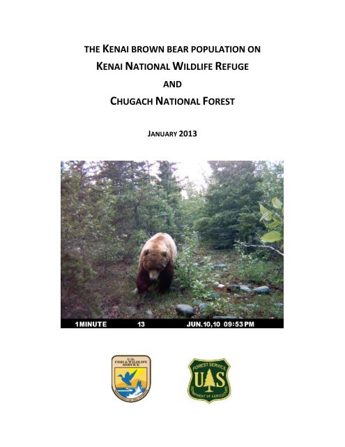
THE KENAI BROWN BEAR POPULATION ON<br />
KENAI NATIONAL WILDLIFE REFUGE<br />
AND<br />
CHUGACH NATIONAL FOREST<br />
JANUARY 2013
THE KENAI BROWN BEAR POPULATION ON<br />
KENAI NATIONAL WILDLIFE REFUGE AND CHUGACH NATIONAL FOREST<br />
January 2013<br />
John M. Mort<strong>on</strong>, Ph.D.<br />
Kenai Nati<strong>on</strong>al <strong>Wildlife</strong> Refuge<br />
U.S. <strong>Fish</strong> <strong>and</strong> <strong>Wildlife</strong> <strong>Service</strong><br />
P.O. Box 2139<br />
Soldotna, AK 99669<br />
907.260.2815, john_m_mort<strong>on</strong>@fws.gov<br />
Martin Bray<br />
Siuslaw Nati<strong>on</strong>al Forest<br />
U.S. Forest <strong>Service</strong><br />
1130 Forestry Lane<br />
Waldport, OR 97394<br />
541.563.8452, martinbray@fs.fed.us<br />
Gregory D. Hayward, Ph.D.<br />
Alaska Regi<strong>on</strong>, U.S. Forest <strong>Service</strong><br />
161 East 1 st Avenue<br />
Anchorage, AK 99501<br />
907.743.9537, ghayward01@fs.fed.us<br />
Gary C. White, Ph.D. (C<strong>on</strong>sultant)<br />
Department of <strong>Fish</strong>, <strong>Wildlife</strong> <strong>and</strong> C<strong>on</strong>servati<strong>on</strong> Biology<br />
Colorado State University<br />
Fort Collins, CO 80523<br />
970.491.6678, gary.white@colostate.edu<br />
David Paetkau, Ph.D. (C<strong>on</strong>sultant)<br />
<strong>Wildlife</strong> Genetics Internati<strong>on</strong>al<br />
P.O. Box 274<br />
Nels<strong>on</strong>, BC V1L5P9 Canada<br />
250.352.3563, dpaetkau@wildlifegenetics.ca<br />
2 | P age
ABSTRACT<br />
Field work for a DNA-based, mark-recapture estimate of <str<strong>on</strong>g>the</str<strong>on</strong>g> Kenai <str<strong>on</strong>g>brown</str<strong>on</strong>g> <str<strong>on</strong>g>bear</str<strong>on</strong>g> <str<strong>on</strong>g>populati<strong>on</strong></str<strong>on</strong>g> <strong>on</strong> <str<strong>on</strong>g>the</str<strong>on</strong>g> Kenai<br />
Nati<strong>on</strong>al <strong>Wildlife</strong> Refuge <strong>and</strong> Chugach Nati<strong>on</strong>al Forest was c<strong>on</strong>ducted during 1 June–1 July 2010. Bears<br />
were attracted to barbed wire stati<strong>on</strong>s deployed in 145 9km x 9km cells systematically distributed across<br />
11,500 km 2 . Using two Bell 206B helicopters <strong>and</strong> four 2-pers<strong>on</strong> field crews, we deployed <str<strong>on</strong>g>the</str<strong>on</strong>g> stati<strong>on</strong>s<br />
during a 6-day period <strong>and</strong> subsequently revisited <str<strong>on</strong>g>the</str<strong>on</strong>g>se stati<strong>on</strong>s <strong>on</strong> 5 c<strong>on</strong>secutive 5-day trap sessi<strong>on</strong>s.<br />
We collected 11,175 hair samples during <str<strong>on</strong>g>the</str<strong>on</strong>g> sessi<strong>on</strong>s from both black <strong>and</strong> <str<strong>on</strong>g>brown</str<strong>on</strong>g> <str<strong>on</strong>g>bear</str<strong>on</strong>g>s, <strong>and</strong> ano<str<strong>on</strong>g>the</str<strong>on</strong>g>r 91<br />
hair samples were collected from o<str<strong>on</strong>g>the</str<strong>on</strong>g>r sources. Extracted DNA was used to identify individual <str<strong>on</strong>g>bear</str<strong>on</strong>g>s<br />
<strong>and</strong> develop capture histories as input to mark-recapture models. Combined with data from ADFGcollared<br />
<str<strong>on</strong>g>bear</str<strong>on</strong>g>s, at least 211 <str<strong>on</strong>g>brown</str<strong>on</strong>g> <str<strong>on</strong>g>bear</str<strong>on</strong>g>s were known to be alive <strong>on</strong> <str<strong>on</strong>g>the</str<strong>on</strong>g> Kenai Peninsula in 2010. AIC<br />
selecti<strong>on</strong> of DNA-based mark-recapture models, based <strong>on</strong> 99 females <strong>and</strong> 104 males, resulted in an<br />
estimate of 428 (95% lognormal CI = 353–539) <str<strong>on</strong>g>brown</str<strong>on</strong>g> <str<strong>on</strong>g>bear</str<strong>on</strong>g>s (including all age classes) <strong>on</strong> <str<strong>on</strong>g>the</str<strong>on</strong>g> study area.<br />
Extrapolating <str<strong>on</strong>g>the</str<strong>on</strong>g> density estimate of 45.1 <str<strong>on</strong>g>bear</str<strong>on</strong>g>s per 1,000 km 2 of available habitat <strong>on</strong> <str<strong>on</strong>g>the</str<strong>on</strong>g> study area to<br />
<str<strong>on</strong>g>the</str<strong>on</strong>g> Kenai Peninsula suggests a peninsula-wide <str<strong>on</strong>g>populati<strong>on</strong></str<strong>on</strong>g> of 624 <str<strong>on</strong>g>brown</str<strong>on</strong>g> <str<strong>on</strong>g>bear</str<strong>on</strong>g>s (95% lognormal CI = 504–<br />
772).<br />
Key words: Alaska, <str<strong>on</strong>g>brown</str<strong>on</strong>g> <str<strong>on</strong>g>bear</str<strong>on</strong>g>, Chugach Nati<strong>on</strong>al Forest, genetics, hair DNA, Kenai Nati<strong>on</strong>al <strong>Wildlife</strong><br />
Refuge, mark-recapture, Pradel model, <str<strong>on</strong>g>populati<strong>on</strong></str<strong>on</strong>g>, Program Mark, Ursus arctos<br />
3 | P age
INTRODUCTION<br />
The grizzly or <str<strong>on</strong>g>brown</str<strong>on</strong>g> <str<strong>on</strong>g>bear</str<strong>on</strong>g> (Ursus arctos) <str<strong>on</strong>g>populati<strong>on</strong></str<strong>on</strong>g> <strong>on</strong> <str<strong>on</strong>g>the</str<strong>on</strong>g> Kenai Peninsula in south-central Alaska is a<br />
keyst<strong>on</strong>e species (IBBST2001). Kenai <str<strong>on</strong>g>brown</str<strong>on</strong>g> <str<strong>on</strong>g>bear</str<strong>on</strong>g>s influence plant distributi<strong>on</strong> <strong>and</strong> abundance through<br />
seed dispersal in feces, transport marine-derived nutrients into terrestrial ecosystems through salm<strong>on</strong><br />
c<strong>on</strong>sumpti<strong>on</strong> (Hilderbr<strong>and</strong> et al. 2005), <strong>and</strong> possibly regulate ungulate <str<strong>on</strong>g>populati<strong>on</strong></str<strong>on</strong>g>s through ne<strong>on</strong>atal<br />
predati<strong>on</strong> under certain c<strong>on</strong>diti<strong>on</strong>s (Zager <strong>and</strong> Beecham 2006). Kenai <str<strong>on</strong>g>brown</str<strong>on</strong>g> <str<strong>on</strong>g>bear</str<strong>on</strong>g>s are recognized as a<br />
source of enjoyment by residents <strong>and</strong> visitors, as a source of revenue for commercial wildlife viewing<br />
<strong>and</strong> hunting charters, <strong>and</strong> as a wilderness ic<strong>on</strong> (ADFG 2000).<br />
The 16-km wide isthmus that separates <str<strong>on</strong>g>the</str<strong>on</strong>g> 24,300 km 2 Kenai Peninsula from <str<strong>on</strong>g>the</str<strong>on</strong>g> adjacent mainl<strong>and</strong><br />
presumably restricts <str<strong>on</strong>g>brown</str<strong>on</strong>g> <str<strong>on</strong>g>bear</str<strong>on</strong>g> emigrati<strong>on</strong> <strong>and</strong> immigrati<strong>on</strong>. Talbot et al. (2009) verified that <str<strong>on</strong>g>the</str<strong>on</strong>g><br />
Kenai <str<strong>on</strong>g>brown</str<strong>on</strong>g> <str<strong>on</strong>g>bear</str<strong>on</strong>g> <str<strong>on</strong>g>populati<strong>on</strong></str<strong>on</strong>g> is indeed insular, significantly differentiated from <str<strong>on</strong>g>the</str<strong>on</strong>g> nearby Anchorage<br />
<str<strong>on</strong>g>brown</str<strong>on</strong>g> <str<strong>on</strong>g>bear</str<strong>on</strong>g> <str<strong>on</strong>g>populati<strong>on</strong></str<strong>on</strong>g> <strong>and</strong> showing less genetic diversity than mainl<strong>and</strong> Alaskan <str<strong>on</strong>g>brown</str<strong>on</strong>g> <str<strong>on</strong>g>bear</str<strong>on</strong>g><br />
<str<strong>on</strong>g>populati<strong>on</strong></str<strong>on</strong>g>s, based <strong>on</strong> both microsatellite loci <strong>and</strong> mitoch<strong>on</strong>drial DNA c<strong>on</strong>trol regi<strong>on</strong> data.<br />
The Kenai Peninsula is also <strong>on</strong>e of <str<strong>on</strong>g>the</str<strong>on</strong>g> fastest urbanizing areas in Alaska, with ~10,000 new residents<br />
added every decade since 1960 (U.S. Census Bureau). Over this same 50-year period, Kenai <str<strong>on</strong>g>brown</str<strong>on</strong>g> <str<strong>on</strong>g>bear</str<strong>on</strong>g>s<br />
killed in defense of life or property (DLP) have increased from
<strong>and</strong> Chugach Nati<strong>on</strong>al Forest. Sec<strong>on</strong>dary objectives included determining <str<strong>on</strong>g>the</str<strong>on</strong>g> sex ratio <strong>and</strong> <str<strong>on</strong>g>the</str<strong>on</strong>g><br />
minimum <str<strong>on</strong>g>brown</str<strong>on</strong>g> <str<strong>on</strong>g>bear</str<strong>on</strong>g> <str<strong>on</strong>g>populati<strong>on</strong></str<strong>on</strong>g> occurring within <str<strong>on</strong>g>the</str<strong>on</strong>g>se two Federal c<strong>on</strong>servati<strong>on</strong> units. We c<strong>on</strong>ducted<br />
our study in June, shortly after <str<strong>on</strong>g>brown</str<strong>on</strong>g> <str<strong>on</strong>g>bear</str<strong>on</strong>g>s have left mostly high-elevati<strong>on</strong> dens (Goldstein et al. 2010)<br />
but before most salm<strong>on</strong> have returned to streams <strong>on</strong> <str<strong>on</strong>g>the</str<strong>on</strong>g> Kenai Peninsula (Jacobs 1989). C<strong>on</strong>sequently,<br />
we included covariates to test our apriori hypo<str<strong>on</strong>g>the</str<strong>on</strong>g>ses that capture rates increased with elevati<strong>on</strong> <strong>and</strong><br />
were unaffected by proximity to anadromous fish streams at this time of year. We tested for geographic<br />
<str<strong>on</strong>g>populati<strong>on</strong></str<strong>on</strong>g> closure by modeling capture rate as functi<strong>on</strong>s of distance to edge of sample frame <strong>and</strong><br />
distance to apparent open edge (Boulanger <strong>and</strong> McLellan 2001). We applied <str<strong>on</strong>g>the</str<strong>on</strong>g> Pradel model (1996) to<br />
fur<str<strong>on</strong>g>the</str<strong>on</strong>g>r test assumpti<strong>on</strong>s of both geographic <strong>and</strong> demographic closure (i.e., negligible change in birth<br />
<strong>and</strong> death rates) during our study.<br />
METHODS<br />
Study area<br />
The Kenai Peninsula juts into <str<strong>on</strong>g>the</str<strong>on</strong>g> Gulf of Alaska, embraced <strong>on</strong> <str<strong>on</strong>g>the</str<strong>on</strong>g> west by <str<strong>on</strong>g>the</str<strong>on</strong>g> Cook Inlet <strong>and</strong> <strong>on</strong> <str<strong>on</strong>g>the</str<strong>on</strong>g> east<br />
by Prince William Sound (Figure 1). Elevati<strong>on</strong>s range from sea level to 2,015 m in <str<strong>on</strong>g>the</str<strong>on</strong>g> Kenai Mountains.<br />
Biodiversity is unusually high for this latitude because of <str<strong>on</strong>g>the</str<strong>on</strong>g> juxtapositi<strong>on</strong> of two biomes <strong>on</strong> <str<strong>on</strong>g>the</str<strong>on</strong>g><br />
peninsula: <str<strong>on</strong>g>the</str<strong>on</strong>g> nor<str<strong>on</strong>g>the</str<strong>on</strong>g>rn fringe of Sitka spruce-dominated (Picea sitchensis) coastal rainforest <strong>on</strong> <str<strong>on</strong>g>the</str<strong>on</strong>g><br />
eastern flank of <str<strong>on</strong>g>the</str<strong>on</strong>g> Kenai Mountains, <strong>and</strong> transiti<strong>on</strong>al boreal forest to <str<strong>on</strong>g>the</str<strong>on</strong>g> west. The latter forest types<br />
include white (P. glauca), black (P. mariana), <strong>and</strong> Lutz (P. X Lutzii) spruces with an admixture of aspen<br />
(Populus tremuloides) <strong>and</strong> birch (Betula neoalaskana)(Table 1). Extensive Sphagnum peatl<strong>and</strong>s are<br />
interspersed am<strong>on</strong>g spruce in <str<strong>on</strong>g>the</str<strong>on</strong>g> Kenai Lowl<strong>and</strong>s. Lichen-dominated tundra replaces mountain<br />
hemlock (Tsuga mertensiana) <strong>and</strong> sub-alpine shrub above treeline.<br />
The study area includes 11,700 km 2 of <str<strong>on</strong>g>the</str<strong>on</strong>g> peninsula <strong>on</strong> l<strong>and</strong>s administered by Kenai Nati<strong>on</strong>al <strong>Wildlife</strong><br />
Refuge <strong>and</strong> Chugach Nati<strong>on</strong>al Forest (Figs. 1,2). The area is bounded in <str<strong>on</strong>g>the</str<strong>on</strong>g> north <strong>and</strong> northwest by<br />
Cook Inlet <strong>and</strong> Turnagain Arm, in <str<strong>on</strong>g>the</str<strong>on</strong>g> east by <str<strong>on</strong>g>the</str<strong>on</strong>g> Sargent Icefield, in <str<strong>on</strong>g>the</str<strong>on</strong>g> south by <str<strong>on</strong>g>the</str<strong>on</strong>g> Harding Icefield<br />
<strong>and</strong> Wosnesenski-Grewingk Glacier complex, <strong>and</strong> in <str<strong>on</strong>g>the</str<strong>on</strong>g> west by Refuge boundaries. The study area<br />
includes 127 (1,390 km) of 250 named streams identified <strong>on</strong> <str<strong>on</strong>g>the</str<strong>on</strong>g> Kenai Peninsula in <str<strong>on</strong>g>the</str<strong>on</strong>g> Catalog of<br />
Waters Important for <str<strong>on</strong>g>the</str<strong>on</strong>g> Spawning, Rearing or Migrati<strong>on</strong> of Anadromous <strong>Fish</strong>es<br />
(http://www.adfg.alaska.gov/sf/SARR/AWC/).<br />
With <str<strong>on</strong>g>the</str<strong>on</strong>g> excepti<strong>on</strong> of <str<strong>on</strong>g>the</str<strong>on</strong>g> southwest corner of <str<strong>on</strong>g>the</str<strong>on</strong>g> peninsula (i.e., south of Caribou Hills), <str<strong>on</strong>g>the</str<strong>on</strong>g> study area<br />
effectively includes all known <strong>and</strong> modeled areas of <str<strong>on</strong>g>brown</str<strong>on</strong>g> <str<strong>on</strong>g>bear</str<strong>on</strong>g> habitati<strong>on</strong> <strong>on</strong> <str<strong>on</strong>g>the</str<strong>on</strong>g> peninsula (IBBST<br />
2001). On average, 87% (SE = 0.03) of 144,024 telemetry locati<strong>on</strong>s from 125 <str<strong>on</strong>g>brown</str<strong>on</strong>g> <str<strong>on</strong>g>bear</str<strong>on</strong>g> adult <strong>and</strong><br />
subadult females radio-collared by <str<strong>on</strong>g>the</str<strong>on</strong>g> IBBST during 1987-2005 were <strong>on</strong> <str<strong>on</strong>g>the</str<strong>on</strong>g> study area (Fig. 3).<br />
Excluding all telemetry locati<strong>on</strong>s collected after 1 July reduces <str<strong>on</strong>g>the</str<strong>on</strong>g> data set to 7,413 locati<strong>on</strong>s from 114<br />
<str<strong>on</strong>g>brown</str<strong>on</strong>g> <str<strong>on</strong>g>bear</str<strong>on</strong>g> females; 11 females (9%) were never <strong>on</strong> <str<strong>on</strong>g>the</str<strong>on</strong>g> sample frame during <str<strong>on</strong>g>the</str<strong>on</strong>g> period when this<br />
study was c<strong>on</strong>ducted. The proporti<strong>on</strong> of telemetry points <strong>on</strong> <str<strong>on</strong>g>the</str<strong>on</strong>g> sample frame, averaged for <str<strong>on</strong>g>the</str<strong>on</strong>g> 114<br />
females, was 84% (SE = 0.03); 75 of 114 females were <strong>on</strong> <str<strong>on</strong>g>the</str<strong>on</strong>g> sample frame during <str<strong>on</strong>g>the</str<strong>on</strong>g> entire sampling<br />
5 | P age
window. Similarly, of 74 <str<strong>on</strong>g>brown</str<strong>on</strong>g> <str<strong>on</strong>g>bear</str<strong>on</strong>g> females for which den sites are known from 1996-2003, 84%<br />
denned at least <strong>on</strong>ce <strong>on</strong> <str<strong>on</strong>g>the</str<strong>on</strong>g> study area (Figure 2).<br />
Study design<br />
We n<strong>on</strong>invasively collected <str<strong>on</strong>g>brown</str<strong>on</strong>g> (<strong>and</strong> black; Ursus americanus) <str<strong>on</strong>g>bear</str<strong>on</strong>g> hairs at barbed-wire stati<strong>on</strong>s<br />
subjectively placed within 145 9km x 9km cells systematically arrayed across <str<strong>on</strong>g>the</str<strong>on</strong>g> study area (Figure 4).<br />
After an initial 6-day deployment period, we employed a rotating panel design in which five panels of 29<br />
cells each were revisited <strong>on</strong> five c<strong>on</strong>secutive 5-day trap sessi<strong>on</strong>s. All cells were visited by two-pers<strong>on</strong><br />
field crews transported by Bell 206-B Jet Ranger helicopters over 31 c<strong>on</strong>secutive days from 1 June–1 July<br />
2010. Field crews <strong>and</strong> helicopters were stati<strong>on</strong>ed in Soldotna <strong>and</strong> Moose Pass (Figure 1).<br />
Using expert judgment (see criteria below), we a priori selected primary <strong>and</strong> sec<strong>on</strong>dary sites within each<br />
cell <strong>on</strong> which to place hair stati<strong>on</strong>s; <str<strong>on</strong>g>the</str<strong>on</strong>g> final coordinates were frequently adjusted in <str<strong>on</strong>g>the</str<strong>on</strong>g> field to better<br />
reflect in situ c<strong>on</strong>diti<strong>on</strong>s. If hair samples were not obtained by <str<strong>on</strong>g>the</str<strong>on</strong>g> end of <str<strong>on</strong>g>the</str<strong>on</strong>g> third trap sessi<strong>on</strong>, we<br />
ei<str<strong>on</strong>g>the</str<strong>on</strong>g>r moved <str<strong>on</strong>g>the</str<strong>on</strong>g> trap to ano<str<strong>on</strong>g>the</str<strong>on</strong>g>r site within <str<strong>on</strong>g>the</str<strong>on</strong>g> cell or added a sec<strong>on</strong>d trap to <str<strong>on</strong>g>the</str<strong>on</strong>g> cell. In additi<strong>on</strong> to<br />
hair samples collected at stati<strong>on</strong>s <strong>on</strong> <str<strong>on</strong>g>the</str<strong>on</strong>g> grid, we supplemented sampling with hair collected at a<br />
permitted black <str<strong>on</strong>g>bear</str<strong>on</strong>g> baiting stati<strong>on</strong> (for hunting), <strong>on</strong> rub trees, <strong>and</strong> from live <str<strong>on</strong>g>bear</str<strong>on</strong>g>s h<strong>and</strong>led during<br />
collaring operati<strong>on</strong>s incidental to this study.<br />
Site selecti<strong>on</strong> for hair sampling stati<strong>on</strong>s<br />
Using GIS, we eliminated all l<strong>and</strong>s from sampling that are restricted by ADFG for black <str<strong>on</strong>g>bear</str<strong>on</strong>g> baiting: no<br />
baiting within 1 mile of any residence, including seas<strong>on</strong>ally occupied dwellings, developed recreati<strong>on</strong>al<br />
facilities or campgrounds; no baiting within 1/4 mile of any publicly-maintained road, trail, or <str<strong>on</strong>g>the</str<strong>on</strong>g> Alaska<br />
Railroad; <strong>and</strong> no baiting within 1/4 mile from <str<strong>on</strong>g>the</str<strong>on</strong>g> shoreline of <str<strong>on</strong>g>the</str<strong>on</strong>g> Kenai, Kasilof <strong>and</strong> Swans<strong>on</strong> Rivers<br />
(including Kenai <strong>and</strong> Skilak Lakes). In total, <str<strong>on</strong>g>the</str<strong>on</strong>g>se buffered (mostly linear) areas c<strong>on</strong>stituted 16% of <str<strong>on</strong>g>the</str<strong>on</strong>g><br />
study area, mostly in relatively high human use areas.<br />
We used <str<strong>on</strong>g>the</str<strong>on</strong>g> following ranked criteria to a priori select two locati<strong>on</strong>s for hair sampling stati<strong>on</strong>s within<br />
each cell from digital ortho quads (DOQs):<br />
1) adequate space for helicopter access;<br />
2) ≥200 m from anthropogenic features (trails, cabins, roads);<br />
3) riparian/wetl<strong>and</strong> corridors associated with stream morphology were given first priority;<br />
4) o<str<strong>on</strong>g>the</str<strong>on</strong>g>r travel corridors c<strong>on</strong>sidered were associated with disc<strong>on</strong>tinuity between vegetati<strong>on</strong><br />
types, avalanche chutes, shoulders between peaks, <strong>and</strong> ridges; <strong>and</strong><br />
5) o<str<strong>on</strong>g>the</str<strong>on</strong>g>r things being equal, trying to ensure spatial separati<strong>on</strong> am<strong>on</strong>g sites within <str<strong>on</strong>g>the</str<strong>on</strong>g> cell.<br />
Hair stati<strong>on</strong>s, sampling <strong>and</strong> processing<br />
Hair was sampled from <str<strong>on</strong>g>bear</str<strong>on</strong>g>s that stepped over or crawled under barbed wire to investigate a simulated<br />
cache laced with lure (Mowat <strong>and</strong> Strobeck 2000). At each stati<strong>on</strong>, we strung two 30-m l<strong>on</strong>g doublestr<strong>and</strong>ed<br />
barbed wires around ≥ 3 trees or rebar stakes to approximate an equilateral triangle at two<br />
6 | P age
heights (20–30 <strong>and</strong> 60–70 cm above ground) to increase <str<strong>on</strong>g>the</str<strong>on</strong>g> likelihood of sampling both adult <str<strong>on</strong>g>bear</str<strong>on</strong>g>s <strong>and</strong><br />
cubs. Logs, rocks, litter, <strong>and</strong> o<str<strong>on</strong>g>the</str<strong>on</strong>g>r debris were piled in <str<strong>on</strong>g>the</str<strong>on</strong>g> center of <str<strong>on</strong>g>the</str<strong>on</strong>g>se hair stati<strong>on</strong>s to simulate a<br />
cache. We used ≥ 3 liters of fermented 3:1 cow blood (The Beef Shop, Centralia, WA) <strong>and</strong> pure,<br />
unprocessed fish oil (Kodiak <strong>Fish</strong> Meal Company), respectively, as lure per stati<strong>on</strong> per visit. O<str<strong>on</strong>g>the</str<strong>on</strong>g>r<br />
substances (e.g., fruit extract, spice oils, anise) were used to augment lures. Signs were posted to both<br />
warn <strong>and</strong> inform public who may have accidentally encountered <str<strong>on</strong>g>the</str<strong>on</strong>g>se sites.<br />
All hair was collected with forceps <strong>and</strong>/or gloves, <strong>and</strong> placed in coin envelopes; <strong>on</strong>e envelope for each<br />
barb cluster. Each coin envelope was bar-coded (Lint<strong>on</strong> Co.) <strong>and</strong> labeled with stati<strong>on</strong> ID, date, barb<br />
number, <strong>and</strong> locati<strong>on</strong> (upper str<strong>and</strong>, lower str<strong>and</strong>). Barbs were burned with a propane torch to remove<br />
any remaining hair after collecti<strong>on</strong>. Any hair <strong>on</strong> <str<strong>on</strong>g>the</str<strong>on</strong>g> ground below barbed wire str<strong>and</strong>s were collected<br />
but not used in <str<strong>on</strong>g>the</str<strong>on</strong>g> analysis. Immediately before leaving, <str<strong>on</strong>g>the</str<strong>on</strong>g> simulated cache was freshened with more<br />
lure.<br />
Hair was dried overnight in opened envelopes if <str<strong>on</strong>g>the</str<strong>on</strong>g> samples were wet at time of collecti<strong>on</strong>. Hair was<br />
stored at room temperature with desiccant. To minimize DNA degradati<strong>on</strong>, hair samples were sent to<br />
<str<strong>on</strong>g>the</str<strong>on</strong>g> lab as so<strong>on</strong> as possible after field work was completed. All unused hair samples (from both <str<strong>on</strong>g>brown</str<strong>on</strong>g><br />
<strong>and</strong> black <str<strong>on</strong>g>bear</str<strong>on</strong>g>s) were archived.<br />
Genetic analysis<br />
Bear species identificati<strong>on</strong>, individual genotyping, <strong>and</strong> sex determinati<strong>on</strong> from DNA in hairs were<br />
c<strong>on</strong>ducted by <strong>Wildlife</strong> Genetics Internati<strong>on</strong>al Inc. (Nels<strong>on</strong>, BC) following quality c<strong>on</strong>trol methods<br />
specified in Paetkau (2003) <strong>and</strong> validated through blind testing by Kendall et al. (2009). To reduce costs,<br />
samples were excluded from genetic analysis if <str<strong>on</strong>g>the</str<strong>on</strong>g>y c<strong>on</strong>tained no guard hairs with roots, <strong>and</strong> < 5<br />
underfur, or if <str<strong>on</strong>g>the</str<strong>on</strong>g>y were clearly from ungulates based <strong>on</strong> appearance. We also excluded over 5,000<br />
guard hair samples that were jet black al<strong>on</strong>g <str<strong>on</strong>g>the</str<strong>on</strong>g>ir entire length, which we felt could be reliably<br />
identified as black <str<strong>on</strong>g>bear</str<strong>on</strong>g> hair in this study area. DNA was extracted from <str<strong>on</strong>g>the</str<strong>on</strong>g> remaining samples using<br />
QIAGEN DNeasy tissue kits, with <str<strong>on</strong>g>the</str<strong>on</strong>g> target of using 10 guard hair roots if available. For guard hairs, we<br />
identified root bulbs under a microscope <strong>and</strong> used <str<strong>on</strong>g>the</str<strong>on</strong>g> bottom 5–10 mm of <str<strong>on</strong>g>the</str<strong>on</strong>g> hair for extracti<strong>on</strong>. For<br />
underfur, where d<strong>and</strong>er caught up in <str<strong>on</strong>g>the</str<strong>on</strong>g> hair can be a significant source of DNA, clumps of hair were<br />
wound toge<str<strong>on</strong>g>the</str<strong>on</strong>g>r <strong>and</strong> placed into <str<strong>on</strong>g>the</str<strong>on</strong>g> first extracti<strong>on</strong> buffer (buffer ATL). In both cases, a warm water<br />
wash was used to remove dirt from <str<strong>on</strong>g>the</str<strong>on</strong>g> hairs before placing <str<strong>on</strong>g>the</str<strong>on</strong>g>m in <str<strong>on</strong>g>the</str<strong>on</strong>g> extracti<strong>on</strong> buffer.<br />
DNA extracts were prescreened with <str<strong>on</strong>g>the</str<strong>on</strong>g> marker G10J, both to weed out weak samples <strong>and</strong> to<br />
separate black <str<strong>on</strong>g>bear</str<strong>on</strong>g> samples from <str<strong>on</strong>g>brown</str<strong>on</strong>g> <str<strong>on</strong>g>bear</str<strong>on</strong>g> samples, based <strong>on</strong> <str<strong>on</strong>g>the</str<strong>on</strong>g> exclusive presence of oddnumbered<br />
allele lengths in <str<strong>on</strong>g>the</str<strong>on</strong>g> former species <strong>and</strong> even-numbered alleles in <str<strong>on</strong>g>the</str<strong>on</strong>g> latter. To identify<br />
individuals, we used 7 microsatellite markers (G1A, G10H, G10J, G1D, G10B, MU50, MU23) with<br />
average heterozygosity > 0.72 in Kenai <str<strong>on</strong>g>brown</str<strong>on</strong>g> <str<strong>on</strong>g>bear</str<strong>on</strong>g>s, as well as an amelogenin sex marker.<br />
The multilocus microsatellite analyses were performed in 3 phases. First, an initial pass was made with all<br />
8 markers, including reanalysis of G10J to c<strong>on</strong>trol for sample h<strong>and</strong>ling errors. Samples that produced solid<br />
7 | P age
data for
streams (DTA). For <str<strong>on</strong>g>the</str<strong>on</strong>g>se variables, we averaged over all captures of an individual. We also c<strong>on</strong>sidered<br />
thresholds of 4.5 <strong>and</strong> 9 km for DTE, <strong>and</strong> 4.5, 9, 18 <strong>and</strong> 27 km for DTOpenE; i.e., <str<strong>on</strong>g>the</str<strong>on</strong>g> values were<br />
truncated when <str<strong>on</strong>g>the</str<strong>on</strong>g> true value exceeded <str<strong>on</strong>g>the</str<strong>on</strong>g>se values. We modeled trapping effort as <str<strong>on</strong>g>the</str<strong>on</strong>g> number of<br />
days of hair trap availability during each of <str<strong>on</strong>g>the</str<strong>on</strong>g> 5 occasi<strong>on</strong>s.<br />
To assess <str<strong>on</strong>g>the</str<strong>on</strong>g> potential for use of Pledger heterogeneity models (Pledger 2005) for <str<strong>on</strong>g>the</str<strong>on</strong>g> 5 trapping<br />
occasi<strong>on</strong>s, a binomial distributi<strong>on</strong> restricted to <str<strong>on</strong>g>the</str<strong>on</strong>g> positive integers (zero-truncated) was fitted to<br />
capture frequencies for females <strong>and</strong> males separately. This model tested whe<str<strong>on</strong>g>the</str<strong>on</strong>g>r <str<strong>on</strong>g>the</str<strong>on</strong>g> observed<br />
frequencies of female <strong>and</strong> male captures could have come from a zero-truncated binomial distributi<strong>on</strong>.<br />
If so, observed heterogeneity was not str<strong>on</strong>g <strong>and</strong> Pledger models were not deemed necessary. If<br />
frequencies did not follow a zero-truncated binomial, Pledger models were deemed necessary <strong>and</strong> were<br />
included during subsequent modeling. Subsequent modeling of <str<strong>on</strong>g>the</str<strong>on</strong>g> combined data set c<strong>on</strong>sidered<br />
detecti<strong>on</strong> probabilities for occasi<strong>on</strong> 0 to be sex-specific, since more females than males carried radio<br />
collars <strong>and</strong> were known to be alive <strong>and</strong> <strong>on</strong> <str<strong>on</strong>g>the</str<strong>on</strong>g> study area. The time-varying models c<strong>on</strong>sidered for<br />
occasi<strong>on</strong>s 1– 5 were c<strong>on</strong>stant capture probabilities across time <strong>and</strong> time-specific capture probabilities.<br />
The basic time-<strong>and</strong>-individual-varying models c<strong>on</strong>sidered for occasi<strong>on</strong>s 1 – 5 were <str<strong>on</strong>g>the</str<strong>on</strong>g> time-varying<br />
models plus a sex effect <strong>and</strong> a sex interacti<strong>on</strong>. In additi<strong>on</strong>, <str<strong>on</strong>g>the</str<strong>on</strong>g> covariates DTE, DTOpenE, ELEV <strong>and</strong> DTA<br />
were added to <str<strong>on</strong>g>the</str<strong>on</strong>g>se models, as well as DTE with thresholds of 4.5 km <strong>and</strong> 9 km <strong>and</strong> DTOpenE with<br />
thresholds of 4.5, 9, 18, <strong>and</strong> 27 km. To evaluate time-specific effects <strong>on</strong> detecti<strong>on</strong> probabilities, a fully<br />
time-specific model with 5 parameters <strong>and</strong> a trapping effort model with 2 parameters were used, with<br />
values of 826, 717, 767, 731, <strong>and</strong> 752 hair-snare days for each of <str<strong>on</strong>g>the</str<strong>on</strong>g> 5 occasi<strong>on</strong>s. The Huggins<br />
c<strong>on</strong>diti<strong>on</strong>al likelihood parameterizati<strong>on</strong> (Huggins 1989, 1991; Alho 1990) was used to estimate<br />
<str<strong>on</strong>g>populati<strong>on</strong></str<strong>on</strong>g> size as a derived parameter:<br />
N ˆ<br />
=<br />
M t<br />
+ 1<br />
∑<br />
i=<br />
1<br />
1−<br />
6<br />
∏<br />
j=<br />
1<br />
1<br />
(1 −<br />
ˆ<br />
p ij<br />
)<br />
All models assume no behavioral effect of capture; i.e., <str<strong>on</strong>g>the</str<strong>on</strong>g> capture probability of <str<strong>on</strong>g>bear</str<strong>on</strong>g>s that have been<br />
detected <strong>on</strong>ce does not change for additi<strong>on</strong>al detecti<strong>on</strong>s. Analyses were c<strong>on</strong>ducted with Program MARK<br />
(White <strong>and</strong> Burnham 1999) using informati<strong>on</strong>-<str<strong>on</strong>g>the</str<strong>on</strong>g>oretic model selecti<strong>on</strong> criteria (AIC c ) <strong>and</strong> model<br />
averaging of <str<strong>on</strong>g>populati<strong>on</strong></str<strong>on</strong>g> estimates (Burnham <strong>and</strong> Anders<strong>on</strong> 2002). AICc weights for Pledger models<br />
were computed for just <str<strong>on</strong>g>the</str<strong>on</strong>g> grid-based hair data to fur<str<strong>on</strong>g>the</str<strong>on</strong>g>r assess <str<strong>on</strong>g>the</str<strong>on</strong>g> need for this mixture model<br />
relative to <str<strong>on</strong>g>the</str<strong>on</strong>g> suite of models c<strong>on</strong>sidered.<br />
To fur<str<strong>on</strong>g>the</str<strong>on</strong>g>r assess <str<strong>on</strong>g>the</str<strong>on</strong>g> assumpti<strong>on</strong>s of both demographic <strong>and</strong> geographic closure, we c<strong>on</strong>structed 4<br />
models with <str<strong>on</strong>g>the</str<strong>on</strong>g> Pradel data type (Pradel 1996) in Program MARK using just <str<strong>on</strong>g>the</str<strong>on</strong>g> 5 hair snare sampling<br />
occasi<strong>on</strong>s. Models c<strong>on</strong>sidered were both apparent survival (φ) <strong>and</strong> fecundity (f) estimated, φ fixed to 1<br />
with f estimated, f fixed to 0 with φ estimated, <strong>and</strong> both φ fixed to 1 <strong>and</strong> f fixed to 0.<br />
9 | P age
RESULTS<br />
Field implementati<strong>on</strong><br />
We originally proposed to sample 190 hair stati<strong>on</strong>s deployed in a systematic grid of 8km x 8km cells.<br />
However, it became very apparent <strong>on</strong> Day 1 (1 June) that we would have trouble completing this sample<br />
design. Although we were deploying stati<strong>on</strong>s in <str<strong>on</strong>g>the</str<strong>on</strong>g> panel closest to fuel depots, <str<strong>on</strong>g>the</str<strong>on</strong>g> Moose Pass <strong>and</strong><br />
Soldotna helicopters logged 6.9 <strong>and</strong> 7.5 hours in flight time, respectively. On Day 2 (2 June), we<br />
decreased <str<strong>on</strong>g>the</str<strong>on</strong>g> number of hair stati<strong>on</strong>s from 190 to 145 by increasing <str<strong>on</strong>g>the</str<strong>on</strong>g> cell size to 9km x 9km.<br />
However, <str<strong>on</strong>g>the</str<strong>on</strong>g> overall spatial footprint of <str<strong>on</strong>g>the</str<strong>on</strong>g> panels was not decreased, <strong>and</strong> it was reflected in flight<br />
times of 7.2 <strong>and</strong> 7.3 hours for <str<strong>on</strong>g>the</str<strong>on</strong>g> Moose Pass <strong>and</strong> Soldotna helicopters, respectively. C<strong>on</strong>sequently, <strong>on</strong><br />
Day 3 (3 June), we completely reshuffled <str<strong>on</strong>g>the</str<strong>on</strong>g> panels, clustering cells around fixed <strong>and</strong> mobile fuel depots<br />
to reduce daily flight time (Figure 4). We had lost irretrievable time by <str<strong>on</strong>g>the</str<strong>on</strong>g>n, so <str<strong>on</strong>g>the</str<strong>on</strong>g> initial deployment of<br />
stati<strong>on</strong>s required 6 (ra<str<strong>on</strong>g>the</str<strong>on</strong>g>r than 5) days, <str<strong>on</strong>g>the</str<strong>on</strong>g>reby extending <str<strong>on</strong>g>the</str<strong>on</strong>g> sampling period through 1 July.<br />
Despite an unusually rainy <strong>and</strong> cold June in 2010, <str<strong>on</strong>g>the</str<strong>on</strong>g> sampling schedule for <str<strong>on</strong>g>the</str<strong>on</strong>g> panels was sustainable<br />
after we established <str<strong>on</strong>g>the</str<strong>on</strong>g> 9 km x 9 km grid array (Figure 4). A stati<strong>on</strong> was never deployed in cell 141<br />
because of persistent snow cover early, <strong>and</strong> poor wea<str<strong>on</strong>g>the</str<strong>on</strong>g>r later in <str<strong>on</strong>g>the</str<strong>on</strong>g> study. Due to a prol<strong>on</strong>ged period<br />
of inclement wea<str<strong>on</strong>g>the</str<strong>on</strong>g>r in Prince William Sound, we were unable to sample 6 cells<br />
(116,135,136,137,145,146) in <str<strong>on</strong>g>the</str<strong>on</strong>g> same panel (Figure 4, panel E) during <str<strong>on</strong>g>the</str<strong>on</strong>g> 2 nd revisit; cell 135 was also<br />
not sampled during <str<strong>on</strong>g>the</str<strong>on</strong>g> 4 th revisit for <str<strong>on</strong>g>the</str<strong>on</strong>g> same reas<strong>on</strong>. Visits to a cell were occasi<strong>on</strong>ally delayed due to<br />
poor wea<str<strong>on</strong>g>the</str<strong>on</strong>g>r or an unusually persistent <str<strong>on</strong>g>bear</str<strong>on</strong>g> but, with <str<strong>on</strong>g>the</str<strong>on</strong>g> excepti<strong>on</strong> of above 6 cells, all cells were<br />
sampled before <str<strong>on</strong>g>the</str<strong>on</strong>g> next scheduled visit.<br />
Hair samples<br />
We collected 11,175 samples of <str<strong>on</strong>g>brown</str<strong>on</strong>g> <strong>and</strong> black <str<strong>on</strong>g>bear</str<strong>on</strong>g> hair from <str<strong>on</strong>g>the</str<strong>on</strong>g> 144 primary stati<strong>on</strong>s <strong>and</strong> 7<br />
sec<strong>on</strong>dary stati<strong>on</strong>s. The 1 st revisit had <str<strong>on</strong>g>the</str<strong>on</strong>g> lowest return (1,550 samples) presumably because trap<br />
sessi<strong>on</strong> length varied from 1–9 days due to modificati<strong>on</strong>s to <str<strong>on</strong>g>the</str<strong>on</strong>g> grid design during <str<strong>on</strong>g>the</str<strong>on</strong>g> first 3 days of<br />
deployment. However, <str<strong>on</strong>g>the</str<strong>on</strong>g> number of samples collected exceeded 2,100 for each of <str<strong>on</strong>g>the</str<strong>on</strong>g> o<str<strong>on</strong>g>the</str<strong>on</strong>g>r 4 revisit<br />
sessi<strong>on</strong>s, each averaging 5 days.<br />
In additi<strong>on</strong> to hair samples collected at hair stati<strong>on</strong>s with lures, 91 samples were collected from rub<br />
trees by USFS staff at Quartz Creek <strong>and</strong> <str<strong>on</strong>g>the</str<strong>on</strong>g> c<strong>on</strong>fluence of <str<strong>on</strong>g>the</str<strong>on</strong>g> Kenai <strong>and</strong> Russian Rivers, <strong>and</strong> by a USFWS<br />
technician who collected samples from his permitted black <str<strong>on</strong>g>bear</str<strong>on</strong>g> baiting stati<strong>on</strong> <strong>on</strong> <str<strong>on</strong>g>the</str<strong>on</strong>g> Kenai Lowl<strong>and</strong>s.<br />
In total, 11,266 hair samples were c<strong>on</strong>sidered in <str<strong>on</strong>g>the</str<strong>on</strong>g>se analyses.<br />
Genotypes<br />
DNA was extracted from 2,671 of 11,266 samples. This subset included 224 extracti<strong>on</strong>s of samples that<br />
were visually classified as black <str<strong>on</strong>g>bear</str<strong>on</strong>g> samples, starting with 50 samples that were extracted specifically<br />
to test <str<strong>on</strong>g>the</str<strong>on</strong>g> visual species identificati<strong>on</strong>s, <strong>and</strong> <str<strong>on</strong>g>the</str<strong>on</strong>g>n adding 174 samples that were extracted at a later<br />
date for an occupancy analysis that will be <str<strong>on</strong>g>the</str<strong>on</strong>g> subject of a future report. Some of <str<strong>on</strong>g>the</str<strong>on</strong>g>se 224 samples<br />
failed during genetic analysis, but <str<strong>on</strong>g>the</str<strong>on</strong>g> successful samples all had odd numbered alleles at G10J,<br />
10 | P age
c<strong>on</strong>firming <str<strong>on</strong>g>the</str<strong>on</strong>g> accuracy of <str<strong>on</strong>g>the</str<strong>on</strong>g> visual species identificati<strong>on</strong>s as black <str<strong>on</strong>g>bear</str<strong>on</strong>g>s. The prescreen process with<br />
marker G10J produced high c<strong>on</strong>fidence, even-numbered scores indicating <str<strong>on</strong>g>brown</str<strong>on</strong>g> <str<strong>on</strong>g>bear</str<strong>on</strong>g>s for 1,226 of<br />
2,671 samples, which went <strong>on</strong> to genotyping with 8 markers. During multilocus genotyping, 1,034<br />
samples produced high-c<strong>on</strong>fidence scores for all 8 markers, <strong>and</strong> were <str<strong>on</strong>g>the</str<strong>on</strong>g>refore used for individual<br />
identificati<strong>on</strong>. There were 211 unique multilocus genotypes represented by <str<strong>on</strong>g>the</str<strong>on</strong>g> 1,034 successful <str<strong>on</strong>g>brown</str<strong>on</strong>g><br />
<str<strong>on</strong>g>bear</str<strong>on</strong>g> samples, of which 166 were identified from hair collected <strong>on</strong> <str<strong>on</strong>g>the</str<strong>on</strong>g> sample frame. Of <str<strong>on</strong>g>the</str<strong>on</strong>g> 211 unique<br />
<str<strong>on</strong>g>brown</str<strong>on</strong>g> <str<strong>on</strong>g>bear</str<strong>on</strong>g>s (i.e., excluding ADFG <str<strong>on</strong>g>bear</str<strong>on</strong>g>s), 47 were detected in ≥ 2 sessi<strong>on</strong>s, 5 were detected in 1 sessi<strong>on</strong><br />
but also identified in o<str<strong>on</strong>g>the</str<strong>on</strong>g>r studies or n<strong>on</strong>study samples, 114 were captured <strong>on</strong>ce, 11 were captured<br />
<strong>on</strong>ly in n<strong>on</strong>study samples, <strong>and</strong> 34 were not captured but previously identified in o<str<strong>on</strong>g>the</str<strong>on</strong>g>r studies or<br />
n<strong>on</strong>study samples.<br />
Based <strong>on</strong> sex <strong>and</strong> perfect matches at 6–9 loci, 32 of <str<strong>on</strong>g>the</str<strong>on</strong>g>se <str<strong>on</strong>g>bear</str<strong>on</strong>g>s were identified as previously h<strong>and</strong>led<br />
<str<strong>on</strong>g>bear</str<strong>on</strong>g>s by ADFG or <str<strong>on</strong>g>the</str<strong>on</strong>g> IBBST. Six of <str<strong>on</strong>g>the</str<strong>on</strong>g> previously h<strong>and</strong>led individuals were males, captured by ADFG or<br />
<str<strong>on</strong>g>the</str<strong>on</strong>g> IBBST during radio-collaring operati<strong>on</strong>s that targeted females. Five of <str<strong>on</strong>g>the</str<strong>on</strong>g> 34 radio-collared <str<strong>on</strong>g>brown</str<strong>on</strong>g><br />
<str<strong>on</strong>g>bear</str<strong>on</strong>g> females (15%) known to be <strong>on</strong> <str<strong>on</strong>g>the</str<strong>on</strong>g> sample frame immediately before or during June 2010 were<br />
matched with genotypes identified by hair sampling.<br />
Species identity was c<strong>on</strong>firmed through a clustering analysis based <strong>on</strong> 6 microsatellite markers,<br />
excluding G10J to ensure independence of tests. Bears with even- <strong>and</strong> odd-numbered G10J alleles<br />
formed 2 discrete clusters, c<strong>on</strong>firming that <str<strong>on</strong>g>the</str<strong>on</strong>g> G10J data had accurately separated species.<br />
Genotyping errors normally create pairs of genotype from <str<strong>on</strong>g>the</str<strong>on</strong>g> same individual that mismatch at 1<br />
marker (Paetkau 2003). Following error-checking <str<strong>on</strong>g>the</str<strong>on</strong>g>re was <strong>on</strong>ly 1 such pair am<strong>on</strong>g <str<strong>on</strong>g>the</str<strong>on</strong>g> 211 <str<strong>on</strong>g>brown</str<strong>on</strong>g> <str<strong>on</strong>g>bear</str<strong>on</strong>g><br />
genotypes that we recognized, <strong>and</strong> this pair was solidly c<strong>on</strong>firmed, first through reanalysis of <str<strong>on</strong>g>the</str<strong>on</strong>g><br />
mismatching marker, <strong>and</strong> <str<strong>on</strong>g>the</str<strong>on</strong>g>n through analysis of 16 additi<strong>on</strong>al markers, several of which mismatched.<br />
There were also 8 pairs of multilocus <str<strong>on</strong>g>brown</str<strong>on</strong>g> <str<strong>on</strong>g>bear</str<strong>on</strong>g> genotypes that matched at 6 of 8 markers, each of<br />
which was c<strong>on</strong>firmed through reanalysis of <str<strong>on</strong>g>the</str<strong>on</strong>g> mismatching markers. Extensive blind testing has shown<br />
that this protocol effectively prevents <str<strong>on</strong>g>the</str<strong>on</strong>g> recogniti<strong>on</strong> of false individuals through genotyping error<br />
(Kendall et al. 2009).<br />
In additi<strong>on</strong> to providing reassurances about genotyping errors, <str<strong>on</strong>g>the</str<strong>on</strong>g> observati<strong>on</strong> of just 1 pair of <str<strong>on</strong>g>brown</str<strong>on</strong>g><br />
<str<strong>on</strong>g>bear</str<strong>on</strong>g>s whose genotypes matched at 7 of 8 markers indicates a low probability that we sampled any pair<br />
of <str<strong>on</strong>g>bear</str<strong>on</strong>g>s with identical 8-locus genotypes. This is because matches at all 8 markers are roughly 10 times<br />
less likely than matches at 7 of 8 markers, just as matches at 6 of 8 markers are more comm<strong>on</strong> than<br />
matches at 7 markers (Paetkau 2003).<br />
Radio-collared female <str<strong>on</strong>g>brown</str<strong>on</strong>g> <str<strong>on</strong>g>bear</str<strong>on</strong>g>s<br />
We located 30 radio-collared female <str<strong>on</strong>g>brown</str<strong>on</strong>g> <str<strong>on</strong>g>bear</str<strong>on</strong>g>s during 5 days of aerial tracking from 26 June–4 July<br />
2010. We combined <str<strong>on</strong>g>the</str<strong>on</strong>g>se locati<strong>on</strong>s with telemetry data received from ADFG in March 2012 which<br />
represented data collected during <str<strong>on</strong>g>the</str<strong>on</strong>g> study but previously unavailable. Toge<str<strong>on</strong>g>the</str<strong>on</strong>g>r <str<strong>on</strong>g>the</str<strong>on</strong>g> samples of radio-<br />
11 | P age
collared female <str<strong>on</strong>g>brown</str<strong>on</strong>g> <str<strong>on</strong>g>bear</str<strong>on</strong>g>s provided geographic locati<strong>on</strong>s of 39 females known to be alive in June<br />
2010 <strong>on</strong> <str<strong>on</strong>g>the</str<strong>on</strong>g> Kenai Peninsula; 5 were not <strong>on</strong> <str<strong>on</strong>g>the</str<strong>on</strong>g> sample frame (Figure 6).<br />
Populati<strong>on</strong> estimati<strong>on</strong><br />
All sources of informati<strong>on</strong> for <str<strong>on</strong>g>brown</str<strong>on</strong>g> <str<strong>on</strong>g>bear</str<strong>on</strong>g>s <strong>on</strong> <str<strong>on</strong>g>the</str<strong>on</strong>g> Kenai Peninsula in June 2010 identified 243 <str<strong>on</strong>g>brown</str<strong>on</strong>g><br />
<str<strong>on</strong>g>bear</str<strong>on</strong>g>s, of which 211 were identified genetically <strong>and</strong> 32 had been h<strong>and</strong>led by ADFG but were not<br />
detected during n<strong>on</strong>-invasive hair sampling. After eliminating <str<strong>on</strong>g>bear</str<strong>on</strong>g>s (n = 40) for which <str<strong>on</strong>g>the</str<strong>on</strong>g>re were no<br />
geographic coordinates, ei<str<strong>on</strong>g>the</str<strong>on</strong>g>r because <str<strong>on</strong>g>the</str<strong>on</strong>g>y were not located (if collared) or were sampled outside <str<strong>on</strong>g>the</str<strong>on</strong>g><br />
study area, we c<strong>on</strong>sidered 203 <str<strong>on</strong>g>bear</str<strong>on</strong>g>s (99 females, 104 males) for analysis. Of <str<strong>on</strong>g>the</str<strong>on</strong>g>se 203 individuals, 65<br />
females <strong>and</strong> 101 males were detected at hair stati<strong>on</strong>s, 5 females <strong>and</strong> 3 males were detected at rub<br />
trees, <strong>and</strong> 29 females were known to be alive <strong>and</strong> <strong>on</strong> <str<strong>on</strong>g>the</str<strong>on</strong>g> sample frame during <str<strong>on</strong>g>the</str<strong>on</strong>g> study period.<br />
Occasi<strong>on</strong> 0 was composed of 41 <str<strong>on</strong>g>brown</str<strong>on</strong>g> <str<strong>on</strong>g>bear</str<strong>on</strong>g>s known to be alive <strong>and</strong> <strong>on</strong> <str<strong>on</strong>g>the</str<strong>on</strong>g> sample frame during <str<strong>on</strong>g>the</str<strong>on</strong>g><br />
study, including 34 collared females <strong>and</strong> 7 <str<strong>on</strong>g>bear</str<strong>on</strong>g>s captured <strong>on</strong> rub trees [note: 1 sow was both collared<br />
<strong>and</strong> detected <strong>on</strong> a rub tree].<br />
Capture frequencies of <str<strong>on</strong>g>the</str<strong>on</strong>g> <str<strong>on</strong>g>bear</str<strong>on</strong>g>s detected <strong>on</strong> <str<strong>on</strong>g>the</str<strong>on</strong>g> sample frame (n = 166) were 3 detecti<strong>on</strong>s (3 females,<br />
5 males), 2 detecti<strong>on</strong>s (17 females, 21 males), <strong>and</strong> 1 detecti<strong>on</strong> (45 females, 75 males). The zerotruncated<br />
binomial fit to <str<strong>on</strong>g>the</str<strong>on</strong>g>se frequencies suggested no lack of fit (P = 0.959 females, P = 0.791 for<br />
males). Fur<str<strong>on</strong>g>the</str<strong>on</strong>g>r, <str<strong>on</strong>g>the</str<strong>on</strong>g> AICc weight for <str<strong>on</strong>g>the</str<strong>on</strong>g> time-specific Pledger model for <str<strong>on</strong>g>the</str<strong>on</strong>g> grid-based hair data was<br />
<strong>on</strong>ly 0.0054, <strong>and</strong> <str<strong>on</strong>g>the</str<strong>on</strong>g> 3-parameter Pledger mixture model (no time variati<strong>on</strong>) received no weight, so<br />
Pledger models were not c<strong>on</strong>sidered in subsequent analyses. With <strong>on</strong>ly 5 occasi<strong>on</strong>s, <str<strong>on</strong>g>the</str<strong>on</strong>g> level of<br />
individual heterogeneity has to be relatively high (i.e., at least a few animals captured <strong>on</strong> all 5 occasi<strong>on</strong>s)<br />
before <str<strong>on</strong>g>the</str<strong>on</strong>g> Pledger mixture models perform reas<strong>on</strong>ably.<br />
Estimates of capture probabilities tended to increase with each successive trap sessi<strong>on</strong> (Table 4) despite<br />
<str<strong>on</strong>g>the</str<strong>on</strong>g> fact that <str<strong>on</strong>g>bear</str<strong>on</strong>g>s were exposed to traps for approximately <str<strong>on</strong>g>the</str<strong>on</strong>g> same time period (~ 5 days) during each<br />
of <str<strong>on</strong>g>the</str<strong>on</strong>g> 5 occasi<strong>on</strong>s. C<strong>on</strong>sequently, model selecti<strong>on</strong> results (Table 2) suggested that a time-specific model<br />
was necessary to explain <str<strong>on</strong>g>the</str<strong>on</strong>g> variati<strong>on</strong> in detecti<strong>on</strong> probabilities for occasi<strong>on</strong>s 1–5, <strong>and</strong> that an additive<br />
sex effect was needed to explain differences between sexes. These effects resulted in <str<strong>on</strong>g>the</str<strong>on</strong>g> base model of<br />
{sex*p(0), sex+p(t)}. ELEV <strong>and</strong> DTE covariates were useful predictors of detecti<strong>on</strong> probabilities when<br />
<str<strong>on</strong>g>the</str<strong>on</strong>g>se covariates were added to <str<strong>on</strong>g>the</str<strong>on</strong>g> base model {sex*p(0), sex+p(t)}, although DTE did not improve up<strong>on</strong><br />
<str<strong>on</strong>g>the</str<strong>on</strong>g> base model. Detecti<strong>on</strong> probabilities declined with ELEV (Figure 7) <strong>and</strong> increased with smaller DTE<br />
values (Figure 8); i.e., <str<strong>on</strong>g>bear</str<strong>on</strong>g>s closer to <str<strong>on</strong>g>the</str<strong>on</strong>g> edge had higher detecti<strong>on</strong> probabilities. When DTA <strong>and</strong><br />
DTOpenE were added to <str<strong>on</strong>g>the</str<strong>on</strong>g> base model {sex*p(0), sex+p(t)}, as well as truncated values of DTE <strong>and</strong><br />
DTOpenE, n<strong>on</strong>e of <str<strong>on</strong>g>the</str<strong>on</strong>g> models produced smaller AIC c values than <str<strong>on</strong>g>the</str<strong>on</strong>g> base model. Model averaging of<br />
<str<strong>on</strong>g>the</str<strong>on</strong>g> <str<strong>on</strong>g>populati<strong>on</strong></str<strong>on</strong>g> estimates (Table 3) suggests that <str<strong>on</strong>g>the</str<strong>on</strong>g>re were 428 (95% lognormal CI = 353–539) <str<strong>on</strong>g>brown</str<strong>on</strong>g><br />
<str<strong>on</strong>g>bear</str<strong>on</strong>g>s of all ages <strong>on</strong> <str<strong>on</strong>g>the</str<strong>on</strong>g> study area in June 2010, of which 215 were females <strong>and</strong> 213 were males.<br />
The model weights for <str<strong>on</strong>g>the</str<strong>on</strong>g> 4 Pradel models c<strong>on</strong>sidered (Table 5) show that 98% of <str<strong>on</strong>g>the</str<strong>on</strong>g> AICc weight is <strong>on</strong><br />
<str<strong>on</strong>g>the</str<strong>on</strong>g> model with φ fixed to 1 <strong>and</strong> f fixed to 0. That is <str<strong>on</strong>g>the</str<strong>on</strong>g> model best supported assumes no emigrati<strong>on</strong> or<br />
12 | P age
immigrati<strong>on</strong>, <strong>and</strong> thus provides fur<str<strong>on</strong>g>the</str<strong>on</strong>g>r evidence that <str<strong>on</strong>g>the</str<strong>on</strong>g> hair snare sampling grid can be assumed<br />
geographically <strong>and</strong> demographically closed.<br />
DISCUSSION<br />
This study produced <str<strong>on</strong>g>the</str<strong>on</strong>g> first empirically-based estimate of <str<strong>on</strong>g>brown</str<strong>on</strong>g> <str<strong>on</strong>g>bear</str<strong>on</strong>g> abundance <strong>on</strong> <str<strong>on</strong>g>the</str<strong>on</strong>g> Kenai<br />
Peninsula, Alaska. As with all <str<strong>on</strong>g>populati<strong>on</strong></str<strong>on</strong>g> estimates of vertebrates in remote locati<strong>on</strong>s, <str<strong>on</strong>g>the</str<strong>on</strong>g> study design<br />
was a compromise am<strong>on</strong>g fiscal c<strong>on</strong>straints, logistics, <strong>and</strong> statistical rigor. The resulting estimate<br />
provides a sound foundati<strong>on</strong> for management agencies <strong>and</strong> o<str<strong>on</strong>g>the</str<strong>on</strong>g>rs to c<strong>on</strong>sider l<strong>and</strong> <strong>and</strong> resource<br />
decisi<strong>on</strong>s. Favorable characteristics of <str<strong>on</strong>g>the</str<strong>on</strong>g> study area combined with a robust survey sample design<br />
al<strong>on</strong>g with careful analysis resulted in an estimate that fit <str<strong>on</strong>g>the</str<strong>on</strong>g> assumpti<strong>on</strong>s for mark-recapture<br />
remarkably well. Despite <str<strong>on</strong>g>the</str<strong>on</strong>g>se strengths, applicati<strong>on</strong> of <str<strong>on</strong>g>the</str<strong>on</strong>g> results will be most effective if certain<br />
characteristics of <str<strong>on</strong>g>the</str<strong>on</strong>g> investigati<strong>on</strong> <strong>and</strong> of <str<strong>on</strong>g>the</str<strong>on</strong>g> modeling process are understood. Below we examine <str<strong>on</strong>g>the</str<strong>on</strong>g><br />
characteristics of our estimate to clarify interpretati<strong>on</strong> of <str<strong>on</strong>g>the</str<strong>on</strong>g> results.<br />
Study design <strong>and</strong> modeling c<strong>on</strong>siderati<strong>on</strong>s<br />
Our study design was similar to that used by Poole et al. (2001) to estimate <str<strong>on</strong>g>the</str<strong>on</strong>g> grizzly <str<strong>on</strong>g>bear</str<strong>on</strong>g> <str<strong>on</strong>g>populati<strong>on</strong></str<strong>on</strong>g><br />
<strong>on</strong> <str<strong>on</strong>g>the</str<strong>on</strong>g> Prophet River in British Columbia. They used a sample frame of 103 9 x 9 km cells <strong>on</strong> an area<br />
slightly smaller than our study area. They used 1 stati<strong>on</strong> within each cell with a single barbed-wire<br />
enclosure, but increased capture rates by moving stati<strong>on</strong>s between each of <str<strong>on</strong>g>the</str<strong>on</strong>g> 5 trap occasi<strong>on</strong>s <strong>and</strong> by<br />
adding new lures. We chose to increase our capture rates by using 2 barbed-wire str<strong>and</strong>s, using<br />
commercial lures in additi<strong>on</strong> to <str<strong>on</strong>g>the</str<strong>on</strong>g> cow blood <strong>and</strong> fish oil lure, <strong>and</strong> adding sec<strong>on</strong>dary stati<strong>on</strong>s or moving<br />
stati<strong>on</strong>s within cells but <strong>on</strong>ly when <str<strong>on</strong>g>the</str<strong>on</strong>g> primary site performed poorly. We also improved our <str<strong>on</strong>g>populati<strong>on</strong></str<strong>on</strong>g><br />
estimate by using supplemental DNA sources: ad hoc sampling of rub trees (Boulanger et al. 2008) <strong>and</strong><br />
telemetry data (Boulanger et al. 2002). We chose to tradeoff intensive sampling with smaller cells<br />
(which may have allowed for <str<strong>on</strong>g>the</str<strong>on</strong>g> detecti<strong>on</strong> <strong>and</strong> modeling of individual heterogeneity; Boulanger et al.<br />
2002) for a more extensive sample frame that encompassed virtually all of <str<strong>on</strong>g>the</str<strong>on</strong>g> known <str<strong>on</strong>g>brown</str<strong>on</strong>g> <str<strong>on</strong>g>bear</str<strong>on</strong>g><br />
habitat <strong>on</strong> <str<strong>on</strong>g>the</str<strong>on</strong>g> Kenai Nati<strong>on</strong>al <strong>Wildlife</strong> Refuge <strong>and</strong> Chugach Nati<strong>on</strong>al Forest, an area that approximates<br />
70% of <str<strong>on</strong>g>the</str<strong>on</strong>g> known <str<strong>on</strong>g>brown</str<strong>on</strong>g> <str<strong>on</strong>g>bear</str<strong>on</strong>g> habitat <strong>on</strong> <str<strong>on</strong>g>the</str<strong>on</strong>g> Kenai Peninsula.<br />
The short trap sessi<strong>on</strong> (5 days), <strong>and</strong> c<strong>on</strong>sequently <str<strong>on</strong>g>the</str<strong>on</strong>g> c<strong>on</strong>strained sampling window (June), makes our<br />
study unique in <str<strong>on</strong>g>the</str<strong>on</strong>g> published literature. Poole et al. (2001) <strong>and</strong> Kendall et al. (2009), for example, used<br />
trap sessi<strong>on</strong>s of 12–14 days. However, both of <str<strong>on</strong>g>the</str<strong>on</strong>g>se <str<strong>on</strong>g>populati<strong>on</strong></str<strong>on</strong>g>s were inl<strong>and</strong> grizzlies, not salm<strong>on</strong>dependent<br />
<str<strong>on</strong>g>brown</str<strong>on</strong>g> <str<strong>on</strong>g>bear</str<strong>on</strong>g>s (Hilderbr<strong>and</strong> et al. 1999). C<strong>on</strong>sequently, although we recognized that shorter<br />
trap sessi<strong>on</strong>s might reduce capture rates, we were c<strong>on</strong>cerned that extending <str<strong>on</strong>g>the</str<strong>on</strong>g> study into July when<br />
most salm<strong>on</strong> return to <str<strong>on</strong>g>the</str<strong>on</strong>g> Kenai Peninsula would reduce both <str<strong>on</strong>g>the</str<strong>on</strong>g> effectiveness of our lures <strong>and</strong> our<br />
study design (because <str<strong>on</strong>g>bear</str<strong>on</strong>g>s begin c<strong>on</strong>gregating al<strong>on</strong>g streams; Figure 8b). To test for this characteristic<br />
of our design, we examined capture rates in relati<strong>on</strong> to salm<strong>on</strong> streams -- as expected (given our spring<br />
trapping), distance to anadromous streams did not significantly improve <str<strong>on</strong>g>the</str<strong>on</strong>g> model (Table 2).<br />
13 | P age
The shorter trap sessi<strong>on</strong>s also limited exposure of samples to <str<strong>on</strong>g>the</str<strong>on</strong>g> elements which can degrade DNA<br />
samples. Our genotyping success was comparatively high (D. Paetkau, pers. comm.). The short trapping<br />
sessi<strong>on</strong> can be particularly important in DNA-sample quality if <str<strong>on</strong>g>the</str<strong>on</strong>g>re is a bias towards samples being<br />
collected shortly after deployment when <str<strong>on</strong>g>the</str<strong>on</strong>g> lure is freshest. Fur<str<strong>on</strong>g>the</str<strong>on</strong>g>rmore, keeping <str<strong>on</strong>g>the</str<strong>on</strong>g> trap sessi<strong>on</strong><br />
short significantly reduced <str<strong>on</strong>g>the</str<strong>on</strong>g> cost of <str<strong>on</strong>g>the</str<strong>on</strong>g> study as <str<strong>on</strong>g>the</str<strong>on</strong>g> two helicopters <strong>and</strong> <str<strong>on</strong>g>the</str<strong>on</strong>g>ir fuel were <str<strong>on</strong>g>the</str<strong>on</strong>g> single<br />
biggest expense. Finally, <str<strong>on</strong>g>the</str<strong>on</strong>g> short sampling window provides reas<strong>on</strong>able assurance of demographic<br />
closure (see below).<br />
Per-occasi<strong>on</strong> capture probabilities in our study did not exceed 0.17 for males <strong>and</strong> 0.11 for females (Table<br />
4). These values were slightly lower than <str<strong>on</strong>g>the</str<strong>on</strong>g> mean capture probability of 0.19 per sessi<strong>on</strong> reported by<br />
Poole et al. (2001) <strong>and</strong> generally lower than <str<strong>on</strong>g>the</str<strong>on</strong>g> observed capture probabilities of 0.1–0.25 reported by<br />
Kendall et al. (2009). The low number of trap occasi<strong>on</strong>s <strong>and</strong> <str<strong>on</strong>g>the</str<strong>on</strong>g> low detecti<strong>on</strong> probabilities have two<br />
negative c<strong>on</strong>sequences. First, <str<strong>on</strong>g>the</str<strong>on</strong>g>se features result in less precise estimates of abundance. Sec<strong>on</strong>d,<br />
<str<strong>on</strong>g>the</str<strong>on</strong>g>se characteristics make it difficult to apply recently-developed Pledger models. We expect individual<br />
heterogeneity of capture probabilities to exist in <str<strong>on</strong>g>the</str<strong>on</strong>g> <str<strong>on</strong>g>populati<strong>on</strong></str<strong>on</strong>g> (i.e., that each animal has its own innate<br />
detecti<strong>on</strong> probability), <strong>and</strong> Pledger models have been dem<strong>on</strong>strated as <str<strong>on</strong>g>the</str<strong>on</strong>g> superior choice for<br />
estimating abundance when capture probabilities are heterogeneous. Unfortunately, <str<strong>on</strong>g>the</str<strong>on</strong>g> Pledger<br />
model, as well as all models that include a comp<strong>on</strong>ent to model individual heterogeneity, performs<br />
poorly when <str<strong>on</strong>g>the</str<strong>on</strong>g> data display little individual heterogeneity <strong>and</strong>/or capture probabilities are low.<br />
Therefore, applicati<strong>on</strong> of Pledger models was not appropriate for our data even though we suspect <str<strong>on</strong>g>the</str<strong>on</strong>g><br />
models fit <str<strong>on</strong>g>the</str<strong>on</strong>g> underlying capture process.<br />
Model selecti<strong>on</strong> with AIC is used in our analyses because of <str<strong>on</strong>g>the</str<strong>on</strong>g> need to recognize uncertainty in which<br />
models should be used to make inference about <str<strong>on</strong>g>the</str<strong>on</strong>g> <str<strong>on</strong>g>populati<strong>on</strong></str<strong>on</strong>g> size (Burnham <strong>and</strong> Anders<strong>on</strong> 2002). A<br />
wide range of models is presented in Table 2. The “best” model is <str<strong>on</strong>g>the</str<strong>on</strong>g> model with <str<strong>on</strong>g>the</str<strong>on</strong>g> smallest, or<br />
minimum, AIC value. However, o<str<strong>on</strong>g>the</str<strong>on</strong>g>r models in Table 2 are “close” to <str<strong>on</strong>g>the</str<strong>on</strong>g> minimum model shown at <str<strong>on</strong>g>the</str<strong>on</strong>g><br />
top of <str<strong>on</strong>g>the</str<strong>on</strong>g> list. To account for uncertainty am<strong>on</strong>g models, we use model averaging, based <strong>on</strong> model AIC<br />
weights shown in Table 2, to obtain an estimate of <str<strong>on</strong>g>populati<strong>on</strong></str<strong>on</strong>g> size. If we chose to <strong>on</strong>ly present <str<strong>on</strong>g>the</str<strong>on</strong>g><br />
estimates from <str<strong>on</strong>g>the</str<strong>on</strong>g> minimum AIC model, we know from <str<strong>on</strong>g>the</str<strong>on</strong>g>ory <strong>and</strong> simulati<strong>on</strong> that <str<strong>on</strong>g>the</str<strong>on</strong>g> c<strong>on</strong>fidence<br />
intervals from this model would be unrealistically narrow because a single model cannot account for <str<strong>on</strong>g>the</str<strong>on</strong>g><br />
model selecti<strong>on</strong> uncertainty. By taking a weighted average of <str<strong>on</strong>g>the</str<strong>on</strong>g> <str<strong>on</strong>g>populati<strong>on</strong></str<strong>on</strong>g> estimates, we have<br />
accounted for model selecti<strong>on</strong> uncertainty in <str<strong>on</strong>g>the</str<strong>on</strong>g> results presented in Table 3.<br />
Lognormal c<strong>on</strong>fidence intervals are presented in Table 3 because of <str<strong>on</strong>g>the</str<strong>on</strong>g> skewness of <str<strong>on</strong>g>the</str<strong>on</strong>g> distributi<strong>on</strong> of<br />
<str<strong>on</strong>g>populati<strong>on</strong></str<strong>on</strong>g> estimates. This is a well established approach that accounts for <str<strong>on</strong>g>the</str<strong>on</strong>g> firm lower bound <strong>on</strong> <str<strong>on</strong>g>the</str<strong>on</strong>g><br />
number of animals in <str<strong>on</strong>g>the</str<strong>on</strong>g> <str<strong>on</strong>g>populati<strong>on</strong></str<strong>on</strong>g> provided by <str<strong>on</strong>g>the</str<strong>on</strong>g> number of individuals known to be alive in <str<strong>on</strong>g>the</str<strong>on</strong>g><br />
<str<strong>on</strong>g>populati<strong>on</strong></str<strong>on</strong>g>. In c<strong>on</strong>trast, <str<strong>on</strong>g>the</str<strong>on</strong>g> upper bound is not c<strong>on</strong>strained <strong>and</strong> results in a l<strong>on</strong>g upper tail <strong>on</strong> <str<strong>on</strong>g>the</str<strong>on</strong>g><br />
sampling distributi<strong>on</strong> of <str<strong>on</strong>g>populati<strong>on</strong></str<strong>on</strong>g> estimates.<br />
14 | P age
Populati<strong>on</strong> estimate <strong>and</strong> model assumpti<strong>on</strong>s<br />
Based <strong>on</strong> 203 individual genotypes, we estimated that 428 <str<strong>on</strong>g>brown</str<strong>on</strong>g> <str<strong>on</strong>g>bear</str<strong>on</strong>g>s were <strong>on</strong> <str<strong>on</strong>g>the</str<strong>on</strong>g> Kenai Nati<strong>on</strong>al<br />
<strong>Wildlife</strong> Refuge <strong>and</strong> Chugach Nati<strong>on</strong>al Forest in June 2010. Although we detected 41% fewer females<br />
than males, model-averaged <str<strong>on</strong>g>populati<strong>on</strong></str<strong>on</strong>g> estimates show essentially <str<strong>on</strong>g>the</str<strong>on</strong>g> same number by sex (Table 3).<br />
The estimate of females is increased c<strong>on</strong>siderably by accounting for <str<strong>on</strong>g>the</str<strong>on</strong>g> females known to be <strong>on</strong> <str<strong>on</strong>g>the</str<strong>on</strong>g><br />
study area but never detected at hair stati<strong>on</strong>s (34 females <strong>and</strong> 3 males were known to be alive <strong>and</strong> <strong>on</strong><br />
<str<strong>on</strong>g>the</str<strong>on</strong>g> study area, but never detected at hair stati<strong>on</strong>s). Model-averaged <str<strong>on</strong>g>populati<strong>on</strong></str<strong>on</strong>g> estimates for females<br />
<strong>and</strong> males from just hair stati<strong>on</strong>s were 114 <strong>and</strong> 194, respectively (Table 3). The difference in <str<strong>on</strong>g>the</str<strong>on</strong>g><br />
estimates from <str<strong>on</strong>g>the</str<strong>on</strong>g> full analysis that included <str<strong>on</strong>g>the</str<strong>on</strong>g> <str<strong>on</strong>g>bear</str<strong>on</strong>g>s known to be <strong>on</strong> <str<strong>on</strong>g>the</str<strong>on</strong>g> study area but never<br />
detected at hair stati<strong>on</strong>s, versus <str<strong>on</strong>g>the</str<strong>on</strong>g> analysis of <strong>on</strong>ly hair-snare detecti<strong>on</strong>s, provides some idea of <str<strong>on</strong>g>the</str<strong>on</strong>g><br />
bias of <str<strong>on</strong>g>the</str<strong>on</strong>g> hair-stati<strong>on</strong> <strong>on</strong>ly data; i.e., not all <str<strong>on</strong>g>bear</str<strong>on</strong>g>s were sampled by hair stati<strong>on</strong>s with equal probability.<br />
For example, Kendall et al. (2009) found that <strong>on</strong>ly 61% of females <strong>and</strong> 35% of males known to be <strong>on</strong><br />
<str<strong>on</strong>g>the</str<strong>on</strong>g>ir study area in nor<str<strong>on</strong>g>the</str<strong>on</strong>g>rn M<strong>on</strong>tana were detected by hair traps. However, <str<strong>on</strong>g>the</str<strong>on</strong>g> inclusi<strong>on</strong> of data from<br />
previously-h<strong>and</strong>led <str<strong>on</strong>g>bear</str<strong>on</strong>g>s (e.g., radio-collared) <strong>on</strong> <str<strong>on</strong>g>the</str<strong>on</strong>g> study area <strong>and</strong> <str<strong>on</strong>g>bear</str<strong>on</strong>g>s detected by rub trees<br />
decreased <str<strong>on</strong>g>the</str<strong>on</strong>g> bias of <str<strong>on</strong>g>the</str<strong>on</strong>g>ir final estimate, just as <str<strong>on</strong>g>the</str<strong>on</strong>g> inclusi<strong>on</strong> here of <str<strong>on</strong>g>bear</str<strong>on</strong>g>s known to be <strong>on</strong> <str<strong>on</strong>g>the</str<strong>on</strong>g> study<br />
area has decreased <str<strong>on</strong>g>the</str<strong>on</strong>g> bias of our estimates.<br />
Our evaluati<strong>on</strong> of capture probabilities resulted in a more pr<strong>on</strong>ounced adjustment for females. Females<br />
of all ages had a lower hair stati<strong>on</strong> detecti<strong>on</strong> probability than males, as shown by Figures 7 <strong>and</strong> 8, <strong>and</strong><br />
dem<strong>on</strong>strated by radio-collared subadult <strong>and</strong> adult females known to be in <str<strong>on</strong>g>the</str<strong>on</strong>g> <str<strong>on</strong>g>populati<strong>on</strong></str<strong>on</strong>g> but never<br />
detected at hair stati<strong>on</strong>s. The model-averaged estimates for females <strong>and</strong> males from just grid-based<br />
detecti<strong>on</strong>s are 114 <strong>and</strong> 194, respectively; with inclusi<strong>on</strong> of <str<strong>on</strong>g>bear</str<strong>on</strong>g>s known to be in <str<strong>on</strong>g>the</str<strong>on</strong>g> <str<strong>on</strong>g>populati<strong>on</strong></str<strong>on</strong>g>, <str<strong>on</strong>g>the</str<strong>on</strong>g><br />
numbers increases to 215 <strong>and</strong> 214. The final estimate for females is almost twice <str<strong>on</strong>g>the</str<strong>on</strong>g> estimate from<br />
grid-based data, whereas <str<strong>on</strong>g>the</str<strong>on</strong>g> estimate for males increases <strong>on</strong>ly ~9%. Females were under-represented<br />
in <str<strong>on</strong>g>the</str<strong>on</strong>g> grid-based sampling presumably because some cohorts may behave differently (e.g., sows with<br />
cubs of <str<strong>on</strong>g>the</str<strong>on</strong>g> year tend to move little during June) <strong>and</strong> because males have almost twice <str<strong>on</strong>g>the</str<strong>on</strong>g> home range<br />
(950 km 2 ) as females (401 km 2 ) <strong>on</strong> <str<strong>on</strong>g>the</str<strong>on</strong>g> Kenai Peninsula (Jacobs 1989). Fur<str<strong>on</strong>g>the</str<strong>on</strong>g>r, <str<strong>on</strong>g>the</str<strong>on</strong>g> presence of 34<br />
females in <str<strong>on</strong>g>the</str<strong>on</strong>g> analysis that were not detected at hair stati<strong>on</strong>s increases <str<strong>on</strong>g>the</str<strong>on</strong>g> number of females known<br />
to be alive <strong>and</strong>, because <str<strong>on</strong>g>the</str<strong>on</strong>g>se 34 <str<strong>on</strong>g>bear</str<strong>on</strong>g>s were undetected, dem<strong>on</strong>strates <str<strong>on</strong>g>the</str<strong>on</strong>g> lower capture probability<br />
of females. Both of <str<strong>on</strong>g>the</str<strong>on</strong>g>se effects result in increasing <str<strong>on</strong>g>the</str<strong>on</strong>g> <str<strong>on</strong>g>populati<strong>on</strong></str<strong>on</strong>g> estimate.<br />
The estimated 50:50 sex ratio that results from our most robust estimate of abundance is unusual in <str<strong>on</strong>g>the</str<strong>on</strong>g><br />
<str<strong>on</strong>g>bear</str<strong>on</strong>g> literature. Grizzly <strong>and</strong> <str<strong>on</strong>g>brown</str<strong>on</strong>g> <str<strong>on</strong>g>bear</str<strong>on</strong>g> studies elsewhere have generally estimated more adult females<br />
than males, typically 60:40; e.g., Pears<strong>on</strong> (1975), Craighead et al. (1974). One possible interpretati<strong>on</strong> is<br />
that our <str<strong>on</strong>g>populati<strong>on</strong></str<strong>on</strong>g> estimate is still biased low for females, even after adjusting <str<strong>on</strong>g>the</str<strong>on</strong>g> modeled estimate<br />
with data from collared <str<strong>on</strong>g>bear</str<strong>on</strong>g>s <strong>and</strong> rub trees. Alternatively, it is also likely that adult female mortality <strong>on</strong><br />
<str<strong>on</strong>g>the</str<strong>on</strong>g> Kenai Peninsula may be skewed high. Unpublished ADFG data from 1967-2011 shows that of 122<br />
adult <str<strong>on</strong>g>brown</str<strong>on</strong>g> <str<strong>on</strong>g>bear</str<strong>on</strong>g>s killed by humans from sources o<str<strong>on</strong>g>the</str<strong>on</strong>g>r than hunting (i.e., DLPs, illegal take, road kills,<br />
<strong>and</strong> management kills), 69% were females. Similarly, an analysis of <str<strong>on</strong>g>the</str<strong>on</strong>g> age structure of 256 <str<strong>on</strong>g>brown</str<strong>on</strong>g> <str<strong>on</strong>g>bear</str<strong>on</strong>g><br />
females captured from 1995–1999 suggested that 2- to 6-year old females were underrepresented in<br />
15 | P age
<str<strong>on</strong>g>the</str<strong>on</strong>g> hypo<str<strong>on</strong>g>the</str<strong>on</strong>g>tical age distributi<strong>on</strong>, a finding that “is troubling because, in o<str<strong>on</strong>g>the</str<strong>on</strong>g>r <str<strong>on</strong>g>brown</str<strong>on</strong>g> <str<strong>on</strong>g>bear</str<strong>on</strong>g> studies,<br />
weaned sub-adult <str<strong>on</strong>g>bear</str<strong>on</strong>g>s usually account for >20% of a <str<strong>on</strong>g>populati<strong>on</strong></str<strong>on</strong>g> “ (IBBST 2001).<br />
We are c<strong>on</strong>fident that <str<strong>on</strong>g>the</str<strong>on</strong>g> assumpti<strong>on</strong> of geographic closure was appropriate for estimating abundance<br />
of this <str<strong>on</strong>g>populati<strong>on</strong></str<strong>on</strong>g>. Distance to edge was originally examined as a covariate to explore <str<strong>on</strong>g>the</str<strong>on</strong>g> potential<br />
violati<strong>on</strong> of geographic closure. Our apriori hypo<str<strong>on</strong>g>the</str<strong>on</strong>g>sis was that detecti<strong>on</strong> probabilities would be lower<br />
for <str<strong>on</strong>g>bear</str<strong>on</strong>g>s near <str<strong>on</strong>g>the</str<strong>on</strong>g> edge because <str<strong>on</strong>g>the</str<strong>on</strong>g>y are likely to spend time outside <str<strong>on</strong>g>the</str<strong>on</strong>g> sample frame (Boulanger <strong>and</strong><br />
McLellan 2001). However, this was not observed <strong>and</strong>, in fact, detecti<strong>on</strong> probabilities were higher closer<br />
to <str<strong>on</strong>g>the</str<strong>on</strong>g> sample frame edge (Figure 7b). We believe this outcome underscores <str<strong>on</strong>g>the</str<strong>on</strong>g> fact that <str<strong>on</strong>g>the</str<strong>on</strong>g> sample<br />
frame was bounded by real geographic barriers <strong>on</strong> ~88% of its 700-km perimeter; i.e., ocean, glaciers,<br />
<str<strong>on</strong>g>the</str<strong>on</strong>g> isthmus (Talbot et al. 2009), <strong>and</strong> <str<strong>on</strong>g>the</str<strong>on</strong>g> urban interface (Suring et al. 1998, Mace et al. 1996), with <strong>on</strong>ly<br />
<str<strong>on</strong>g>the</str<strong>on</strong>g> southwest corner of <str<strong>on</strong>g>the</str<strong>on</strong>g> grid open to significant immigrati<strong>on</strong>/emigrati<strong>on</strong> from a small area south of<br />
Caribou Hills (Figure 4). Bears traveling al<strong>on</strong>g <str<strong>on</strong>g>the</str<strong>on</strong>g>se barriers may move al<strong>on</strong>g <str<strong>on</strong>g>the</str<strong>on</strong>g> perimeter because<br />
<str<strong>on</strong>g>the</str<strong>on</strong>g>y cannot (in <str<strong>on</strong>g>the</str<strong>on</strong>g> case of <str<strong>on</strong>g>the</str<strong>on</strong>g> former) or prefer not (in <str<strong>on</strong>g>the</str<strong>on</strong>g> case of <str<strong>on</strong>g>the</str<strong>on</strong>g> latter) to move through it. As a<br />
c<strong>on</strong>sequence, <str<strong>on</strong>g>the</str<strong>on</strong>g>se <str<strong>on</strong>g>bear</str<strong>on</strong>g>s encounter more stati<strong>on</strong>s near <str<strong>on</strong>g>the</str<strong>on</strong>g> edge of <str<strong>on</strong>g>the</str<strong>on</strong>g> sample frame. Regardless of<br />
<str<strong>on</strong>g>the</str<strong>on</strong>g> explanati<strong>on</strong>, evidence for an edge effect is weak (Figure 7b), <strong>and</strong> <str<strong>on</strong>g>the</str<strong>on</strong>g> threshold models for DTE were<br />
not highly ranked models (Table 2). We explored <str<strong>on</strong>g>the</str<strong>on</strong>g> influence of <str<strong>on</strong>g>the</str<strong>on</strong>g> dominant ‘open boundary’<br />
through a series of models labeled DTOpenE. Models exploring <str<strong>on</strong>g>the</str<strong>on</strong>g> influence of this edge ( DTOpenE)<br />
were even less supported than <str<strong>on</strong>g>the</str<strong>on</strong>g> DTE models based <strong>on</strong> <str<strong>on</strong>g>the</str<strong>on</strong>g> AICc weights in Table 2. Finally, <str<strong>on</strong>g>the</str<strong>on</strong>g> Pradel<br />
model which assumes closure was <str<strong>on</strong>g>the</str<strong>on</strong>g> most supported model with 98% of <str<strong>on</strong>g>the</str<strong>on</strong>g> AICc weight. Thus, a<br />
range of evidence suggests that analysis with models that assume geographic closure was a reas<strong>on</strong>able<br />
choice for <str<strong>on</strong>g>the</str<strong>on</strong>g> <str<strong>on</strong>g>populati<strong>on</strong></str<strong>on</strong>g> – potentially more so than in many mark-recapture investigati<strong>on</strong>s.<br />
Demographic closure is ano<str<strong>on</strong>g>the</str<strong>on</strong>g>r potential c<strong>on</strong>cern for mark-recapture estimates. Violati<strong>on</strong> of<br />
demographic closure might occur if a proporti<strong>on</strong> of <str<strong>on</strong>g>the</str<strong>on</strong>g> <str<strong>on</strong>g>populati<strong>on</strong></str<strong>on</strong>g> were to die during <str<strong>on</strong>g>the</str<strong>on</strong>g> study. Study<br />
design which emphasized a short sample period in <str<strong>on</strong>g>the</str<strong>on</strong>g> spring suggests this would not be a problem. A<br />
sec<strong>on</strong>d violati<strong>on</strong> of <str<strong>on</strong>g>the</str<strong>on</strong>g> demographic closure assumpti<strong>on</strong> could occur if cubs of <str<strong>on</strong>g>the</str<strong>on</strong>g> year were sampled<br />
more frequently as <str<strong>on</strong>g>the</str<strong>on</strong>g> study progressed or perhaps not at all. However, we doubt <str<strong>on</strong>g>the</str<strong>on</strong>g> former was <str<strong>on</strong>g>the</str<strong>on</strong>g><br />
case as sows with young of <str<strong>on</strong>g>the</str<strong>on</strong>g> year tend to stay near <str<strong>on</strong>g>the</str<strong>on</strong>g>ir natal sites, particularly early in <str<strong>on</strong>g>the</str<strong>on</strong>g> summer<br />
when this study was c<strong>on</strong>ducted. In <str<strong>on</strong>g>the</str<strong>on</strong>g> case of <str<strong>on</strong>g>the</str<strong>on</strong>g> latter, we chose to use 2 barbed wires strung at<br />
different heights as a reas<strong>on</strong>able way to ensure that cubs were sampled. Although inclusi<strong>on</strong> of cubs in<br />
estimates using single barbed wire has been suggested in various studies (Boulanger et al. 2004, Kendall<br />
et al. 2009), <strong>and</strong> Boulanger et al. (2006) did not show large differences in estimates from single- versus<br />
double-str<strong>and</strong> enclosures, we also recognized that <str<strong>on</strong>g>the</str<strong>on</strong>g> size range of Kenai <str<strong>on</strong>g>brown</str<strong>on</strong>g> <str<strong>on</strong>g>bear</str<strong>on</strong>g>s is much greater<br />
than in interior grizzly <str<strong>on</strong>g>populati<strong>on</strong></str<strong>on</strong>g>s. This attribute makes it more difficult to assume that a single str<strong>and</strong><br />
would suffice for all sizes.<br />
Multiple captures of different genotypes tended to NOT occur in <str<strong>on</strong>g>the</str<strong>on</strong>g> Kenai Lowl<strong>and</strong>s in <str<strong>on</strong>g>the</str<strong>on</strong>g> nor<str<strong>on</strong>g>the</str<strong>on</strong>g>ast<br />
quarter of <str<strong>on</strong>g>the</str<strong>on</strong>g> same frame (Figure 5), <strong>and</strong> thus provides perspective <strong>on</strong> <str<strong>on</strong>g>the</str<strong>on</strong>g> spatial distributi<strong>on</strong> of <str<strong>on</strong>g>bear</str<strong>on</strong>g><br />
density. This area of <str<strong>on</strong>g>the</str<strong>on</strong>g> sample frame has <str<strong>on</strong>g>the</str<strong>on</strong>g> lowest elevati<strong>on</strong> as well, <strong>and</strong> would thus seem<br />
somewhat inc<strong>on</strong>sistent with <str<strong>on</strong>g>the</str<strong>on</strong>g> inverse relati<strong>on</strong>ship between ELEV <strong>and</strong> detecti<strong>on</strong> probability (Figure<br />
16 | P age
7a). However, a retrospective analyses of 46 GPS-collared Kenai <str<strong>on</strong>g>brown</str<strong>on</strong>g> <str<strong>on</strong>g>bear</str<strong>on</strong>g> females show <str<strong>on</strong>g>the</str<strong>on</strong>g>y move<br />
most in June (Figure 8a) <strong>and</strong> are fur<str<strong>on</strong>g>the</str<strong>on</strong>g>st away from streams in June (Figure 8b). This is c<strong>on</strong>sistent with<br />
our c<strong>on</strong>ceptual model that most Kenai <str<strong>on</strong>g>brown</str<strong>on</strong>g> <str<strong>on</strong>g>bear</str<strong>on</strong>g>s emerge in <str<strong>on</strong>g>the</str<strong>on</strong>g> spring from steeped-slope, highelevati<strong>on</strong><br />
dens (Figure 2) through mid-May (Goldstein et al. 2010), move quickly towards lowerelevati<strong>on</strong><br />
calving areas for moose, <strong>and</strong> <str<strong>on</strong>g>the</str<strong>on</strong>g>n move towards streams as <str<strong>on</strong>g>the</str<strong>on</strong>g> early runs of chinook <strong>and</strong><br />
sockeye salm<strong>on</strong> enter streams in late June (Jacobs 1989). The excepti<strong>on</strong> is sows with cubs of <str<strong>on</strong>g>the</str<strong>on</strong>g> year, a<br />
cohort that will tend to remain at higher elevati<strong>on</strong>s near natal sites during early summer (IBBST 2001).<br />
This gradual movement across <str<strong>on</strong>g>the</str<strong>on</strong>g> study area, combined with <str<strong>on</strong>g>the</str<strong>on</strong>g> observed lower detecti<strong>on</strong> probabilities<br />
for <str<strong>on</strong>g>the</str<strong>on</strong>g> early occasi<strong>on</strong>s <strong>and</strong> higher detecti<strong>on</strong> probabilities in <str<strong>on</strong>g>the</str<strong>on</strong>g> later occasi<strong>on</strong>s (Table 4) would explain<br />
why we found higher detecti<strong>on</strong> probabilities at lower elevati<strong>on</strong>s. Bears were at lower elevati<strong>on</strong>s during<br />
<str<strong>on</strong>g>the</str<strong>on</strong>g> later occasi<strong>on</strong>s of <str<strong>on</strong>g>the</str<strong>on</strong>g> survey, providing higher detecti<strong>on</strong> probabilities. The observed weak<br />
relati<strong>on</strong>ships of DTE <strong>and</strong> ELEV to capture probabilities (Figs. 7a, 7b) make more sense in this light.<br />
Models c<strong>on</strong>sidered but discarded<br />
As noted earlier, <str<strong>on</strong>g>the</str<strong>on</strong>g> design of this study <strong>and</strong> <str<strong>on</strong>g>the</str<strong>on</strong>g> pattern of recaptures lead to a c<strong>on</strong>cern that capture<br />
heterogeneity was not being modeled well resulting in poor estimati<strong>on</strong> of precisi<strong>on</strong>. We c<strong>on</strong>sidered<br />
several opti<strong>on</strong>s to address this issue. We carefully c<strong>on</strong>sidered <str<strong>on</strong>g>the</str<strong>on</strong>g> Pledger mixture model but ultimately<br />
c<strong>on</strong>cluded this approach is not appropriate for our circumstances where multiple <str<strong>on</strong>g>bear</str<strong>on</strong>g>s were known to<br />
be <strong>on</strong> <str<strong>on</strong>g>the</str<strong>on</strong>g> sample frame, but never detected at <str<strong>on</strong>g>the</str<strong>on</strong>g> hair sampling stati<strong>on</strong>s. Data from radio-collared<br />
<str<strong>on</strong>g>bear</str<strong>on</strong>g>s makes it clear that numerous <str<strong>on</strong>g>bear</str<strong>on</strong>g>s with no encounters occurred <strong>on</strong> <str<strong>on</strong>g>the</str<strong>on</strong>g> grid in June 2010;<br />
C<strong>on</strong>sequently <str<strong>on</strong>g>the</str<strong>on</strong>g>ir hair stati<strong>on</strong> encounter history is all zeros. That is, we included 41 <str<strong>on</strong>g>bear</str<strong>on</strong>g>s known to be<br />
alive <strong>and</strong> <strong>on</strong> <str<strong>on</strong>g>the</str<strong>on</strong>g> grid during sampling, of which <strong>on</strong>ly 4 were detected at <str<strong>on</strong>g>the</str<strong>on</strong>g> hair stati<strong>on</strong>s; thus, 37 <str<strong>on</strong>g>bear</str<strong>on</strong>g>s<br />
had an encounter history of 100000. The Pledger mixture model evaluates this capture history <strong>and</strong><br />
estimates probability of capture for this set as very near zero. When <str<strong>on</strong>g>the</str<strong>on</strong>g> count of <str<strong>on</strong>g>bear</str<strong>on</strong>g>s is divided by this<br />
estimated capture probability (~ zero) <str<strong>on</strong>g>the</str<strong>on</strong>g> resulting <str<strong>on</strong>g>populati<strong>on</strong></str<strong>on</strong>g> estimate will be near infinity. Thus, <str<strong>on</strong>g>the</str<strong>on</strong>g><br />
Pledger mixture model cannot be applied to <str<strong>on</strong>g>the</str<strong>on</strong>g> hair-snare encounters in our situati<strong>on</strong>.<br />
Spatially-explicit capture-recapture (SECR) models represent a recent development in estimators that is<br />
especially suitable when geographic closure is a c<strong>on</strong>cern. We did not use SECR models for 3 reas<strong>on</strong>s.<br />
Foremost, SECR models would not have accommodated data for <str<strong>on</strong>g>the</str<strong>on</strong>g> <str<strong>on</strong>g>bear</str<strong>on</strong>g>s known to be alive <strong>and</strong> <strong>on</strong> <str<strong>on</strong>g>the</str<strong>on</strong>g><br />
grid, but never detected in hair samples. As discussed above, improvements in estimates of capture<br />
probabilities achieved by including <str<strong>on</strong>g>the</str<strong>on</strong>g>se <str<strong>on</strong>g>bear</str<strong>on</strong>g>s in <str<strong>on</strong>g>the</str<strong>on</strong>g> study are substantial. Without informati<strong>on</strong><br />
provided by <str<strong>on</strong>g>the</str<strong>on</strong>g>se <str<strong>on</strong>g>bear</str<strong>on</strong>g>s our estimates would suggest an extremely skewed sex ratio (with males<br />
dominating). Sec<strong>on</strong>d, SECR models result in an estimate of <str<strong>on</strong>g>bear</str<strong>on</strong>g> density ra<str<strong>on</strong>g>the</str<strong>on</strong>g>r than abundance.<br />
Producing an estimate of abundance is accomplished by multiplying <str<strong>on</strong>g>the</str<strong>on</strong>g> estimated density by <str<strong>on</strong>g>the</str<strong>on</strong>g> size of<br />
<str<strong>on</strong>g>the</str<strong>on</strong>g> study area. This results in <str<strong>on</strong>g>the</str<strong>on</strong>g> problem familiar to all practiti<strong>on</strong>ers of mark-recapture modeling –<br />
determining <str<strong>on</strong>g>the</str<strong>on</strong>g> size of <str<strong>on</strong>g>the</str<strong>on</strong>g> sample area. For <str<strong>on</strong>g>the</str<strong>on</strong>g> SECR models, <str<strong>on</strong>g>the</str<strong>on</strong>g> issue includes problems associated<br />
with <str<strong>on</strong>g>bear</str<strong>on</strong>g>s using <str<strong>on</strong>g>the</str<strong>on</strong>g> sample area but whose home range center does not occur in <str<strong>on</strong>g>the</str<strong>on</strong>g> study area.<br />
Finally, we rejected SECR models because of issues estimating σ (a parameter associated with home<br />
range size) based <strong>on</strong> our capture histories. To rigorously estimate σ, SECR models use recapture<br />
histories, representing movements of <str<strong>on</strong>g>bear</str<strong>on</strong>g>s am<strong>on</strong>g snare sites. Our data included <strong>on</strong>ly 54 pairs of<br />
17 | P age
distances from which to estimate movements. Fur<str<strong>on</strong>g>the</str<strong>on</strong>g>r, σ should be estimated separately for male <strong>and</strong><br />
female <str<strong>on</strong>g>bear</str<strong>on</strong>g>s, because of <str<strong>on</strong>g>the</str<strong>on</strong>g> well-documented differences in home range size of <str<strong>on</strong>g>the</str<strong>on</strong>g> sexes. SECR<br />
models developed with limited data generally require biologically unrealistic assumpti<strong>on</strong> of a circular<br />
area-of-activity. During June, <str<strong>on</strong>g>bear</str<strong>on</strong>g>s <strong>on</strong> <str<strong>on</strong>g>the</str<strong>on</strong>g> Kenai are known to move directi<strong>on</strong>ally from dens toward<br />
moose calving areas suggesting a circular activity area is not a reas<strong>on</strong>able assumpti<strong>on</strong>. For <str<strong>on</strong>g>the</str<strong>on</strong>g>se<br />
reas<strong>on</strong>s, we rejected SECR models as a str<strong>on</strong>ger approach to estimating <str<strong>on</strong>g>bear</str<strong>on</strong>g>s from <str<strong>on</strong>g>the</str<strong>on</strong>g> data collected in<br />
this study.<br />
Ivan et al. (2-13a, b) describe an alternative, spatial modeling approach to examine mark-recapture data.<br />
In c<strong>on</strong>trast to <str<strong>on</strong>g>the</str<strong>on</strong>g> SECR approach, <str<strong>on</strong>g>the</str<strong>on</strong>g> method defines explicit study boundaries <strong>and</strong> thus eliminates <str<strong>on</strong>g>the</str<strong>on</strong>g><br />
problem of estimating abundance (from <str<strong>on</strong>g>the</str<strong>on</strong>g> density estimate) encountered with SECR models.<br />
However, this estimator requires that animals be m<strong>on</strong>itored for use of <str<strong>on</strong>g>the</str<strong>on</strong>g> sample frame before <strong>and</strong><br />
after <str<strong>on</strong>g>the</str<strong>on</strong>g> lure is removed. Typically this m<strong>on</strong>itoring requires that animals be radio-collared when<br />
captured <strong>on</strong> <str<strong>on</strong>g>the</str<strong>on</strong>g> sample frame <strong>and</strong> <str<strong>on</strong>g>the</str<strong>on</strong>g>n m<strong>on</strong>itored after <str<strong>on</strong>g>the</str<strong>on</strong>g> capture-recapture porti<strong>on</strong> of <str<strong>on</strong>g>the</str<strong>on</strong>g> study is<br />
completed. In our case, we were not specifically capturing animals <strong>on</strong> our sample frame, <strong>and</strong> so do not<br />
have a legitimate sample of <str<strong>on</strong>g>the</str<strong>on</strong>g> <str<strong>on</strong>g>bear</str<strong>on</strong>g>s detected via hair snares to <str<strong>on</strong>g>the</str<strong>on</strong>g>n m<strong>on</strong>itor for use of <str<strong>on</strong>g>the</str<strong>on</strong>g> grid later.<br />
Fur<str<strong>on</strong>g>the</str<strong>on</strong>g>r, <str<strong>on</strong>g>the</str<strong>on</strong>g> estimator of Ivan et al. assumes that animals do not change <str<strong>on</strong>g>the</str<strong>on</strong>g>ir home ranges after<br />
trapping is completed. This assumpti<strong>on</strong> is likely not appropriate for our study where <str<strong>on</strong>g>bear</str<strong>on</strong>g>s were moving<br />
from den sites during June <strong>and</strong> likely changing <str<strong>on</strong>g>the</str<strong>on</strong>g> areas used over <str<strong>on</strong>g>the</str<strong>on</strong>g> course of <str<strong>on</strong>g>the</str<strong>on</strong>g> summer.<br />
Management implicati<strong>on</strong>s<br />
We employed sophisticated models to estimate <str<strong>on</strong>g>brown</str<strong>on</strong>g> <str<strong>on</strong>g>bear</str<strong>on</strong>g> abundance <strong>on</strong> <str<strong>on</strong>g>the</str<strong>on</strong>g> Kenai Peninsula using a<br />
combinati<strong>on</strong> of n<strong>on</strong>-invasive DNA sampling <strong>and</strong> informati<strong>on</strong> <strong>on</strong> radio-collared <str<strong>on</strong>g>bear</str<strong>on</strong>g>s using markrecapture<br />
estimators. Based <strong>on</strong> an underst<strong>and</strong>ing of <str<strong>on</strong>g>bear</str<strong>on</strong>g> biology, <str<strong>on</strong>g>the</str<strong>on</strong>g> pattern of recaptures, <strong>and</strong> <str<strong>on</strong>g>the</str<strong>on</strong>g><br />
characteristics of <str<strong>on</strong>g>the</str<strong>on</strong>g> study area, we are c<strong>on</strong>fident that our approach did not suffer from c<strong>on</strong>founding<br />
issues of geographic closure or demographic closure. However, it is clear from <str<strong>on</strong>g>the</str<strong>on</strong>g> data that female<br />
<str<strong>on</strong>g>bear</str<strong>on</strong>g>s had very low recapture probabilities <strong>and</strong> it is likely that <str<strong>on</strong>g>bear</str<strong>on</strong>g>s from both sexes had variable<br />
recapture probabilities. Therefore, based <strong>on</strong> an underst<strong>and</strong>ing of <str<strong>on</strong>g>the</str<strong>on</strong>g> performance of our estimators,<br />
we suggest that both <str<strong>on</strong>g>the</str<strong>on</strong>g> point estimate of <str<strong>on</strong>g>bear</str<strong>on</strong>g> abundance (428 <str<strong>on</strong>g>brown</str<strong>on</strong>g> <str<strong>on</strong>g>bear</str<strong>on</strong>g>s) <strong>and</strong> <str<strong>on</strong>g>the</str<strong>on</strong>g> precisi<strong>on</strong> of our<br />
estimate (95% lognormal CI = 353–539) are likely biased low. This means that, given <str<strong>on</strong>g>the</str<strong>on</strong>g> known<br />
performance of our estimati<strong>on</strong> approach, <str<strong>on</strong>g>the</str<strong>on</strong>g> true number of <str<strong>on</strong>g>brown</str<strong>on</strong>g> <str<strong>on</strong>g>bear</str<strong>on</strong>g>s <strong>on</strong> our sample area in June<br />
2010 was more likely to be above our point estimate than below. Fur<str<strong>on</strong>g>the</str<strong>on</strong>g>rmore, <str<strong>on</strong>g>the</str<strong>on</strong>g> ‘true’ 95% CI is likely<br />
to be broader than our estimate. These characteristics do not undermine our estimate; ra<str<strong>on</strong>g>the</str<strong>on</strong>g>r, we<br />
highlight <str<strong>on</strong>g>the</str<strong>on</strong>g>se characteristics so that managers make decisi<strong>on</strong>s with a clear underst<strong>and</strong>ing of <str<strong>on</strong>g>the</str<strong>on</strong>g> nature<br />
of <str<strong>on</strong>g>the</str<strong>on</strong>g> estimate.<br />
Our estimate of <str<strong>on</strong>g>the</str<strong>on</strong>g> Kenai <str<strong>on</strong>g>brown</str<strong>on</strong>g> <str<strong>on</strong>g>bear</str<strong>on</strong>g> <str<strong>on</strong>g>populati<strong>on</strong></str<strong>on</strong>g> is generally c<strong>on</strong>sistent with estimates of <str<strong>on</strong>g>brown</str<strong>on</strong>g> <str<strong>on</strong>g>bear</str<strong>on</strong>g><br />
density in interior, ra<str<strong>on</strong>g>the</str<strong>on</strong>g>r than coastal, Alaska (but see Flynn et al. 2012). Available habitat <strong>on</strong> <str<strong>on</strong>g>the</str<strong>on</strong>g><br />
sample frame, after subtracting <str<strong>on</strong>g>the</str<strong>on</strong>g> Harding Icefield, water bodies, <strong>and</strong> <str<strong>on</strong>g>the</str<strong>on</strong>g> anthropogenic footprint,<br />
approximates 9,500 km 2 , translating to a mean <str<strong>on</strong>g>brown</str<strong>on</strong>g> <str<strong>on</strong>g>bear</str<strong>on</strong>g> density of 45.1 per 1,000 km 2 . To put this in<br />
perspective, Miller et al. (1997) reported <str<strong>on</strong>g>brown</str<strong>on</strong>g> <str<strong>on</strong>g>bear</str<strong>on</strong>g> densities (all ages) <strong>on</strong> 7 study sites in sou<str<strong>on</strong>g>the</str<strong>on</strong>g>rn<br />
18 | P age
coastal habitats of Alaska that were characterized by abundant runs of multiple salm<strong>on</strong> species; <str<strong>on</strong>g>the</str<strong>on</strong>g>se<br />
estimates for coastal <str<strong>on</strong>g>bear</str<strong>on</strong>g> <str<strong>on</strong>g>populati<strong>on</strong></str<strong>on</strong>g>s ranged from 191–551 per 1,000 km 2 . In c<strong>on</strong>trast, <str<strong>on</strong>g>brown</str<strong>on</strong>g> <str<strong>on</strong>g>bear</str<strong>on</strong>g><br />
densities (all ages) <strong>on</strong> 11 study sites in interior Alaska ranged from 10–30 per 1,000 km 2 (Figure 9). Our<br />
estimate places <str<strong>on</strong>g>the</str<strong>on</strong>g> Kenai <str<strong>on</strong>g>populati<strong>on</strong></str<strong>on</strong>g> within <str<strong>on</strong>g>the</str<strong>on</strong>g> lower (
CI = 0.9364–1.0588) for 1995–99 (IBBST 2001); <str<strong>on</strong>g>the</str<strong>on</strong>g> c<strong>on</strong>fidence bounds make it difficult to determine <str<strong>on</strong>g>the</str<strong>on</strong>g><br />
<str<strong>on</strong>g>populati<strong>on</strong></str<strong>on</strong>g> trajectory but suggest a stable <str<strong>on</strong>g>populati<strong>on</strong></str<strong>on</strong>g>. However, a recent unpublished λ estimate of<br />
1.039 (95% CI = 1.036–1.043) for 1995–2011 (Farley 2011) suggests that <str<strong>on</strong>g>the</str<strong>on</strong>g> <str<strong>on</strong>g>populati<strong>on</strong></str<strong>on</strong>g> may be<br />
increasing.<br />
C<strong>on</strong>clusi<strong>on</strong><br />
This DNA-based mark-recapture estimati<strong>on</strong> of <str<strong>on</strong>g>the</str<strong>on</strong>g> Kenai <str<strong>on</strong>g>brown</str<strong>on</strong>g> <str<strong>on</strong>g>bear</str<strong>on</strong>g> <str<strong>on</strong>g>populati<strong>on</strong></str<strong>on</strong>g> was unc<strong>on</strong>venti<strong>on</strong>ally<br />
short in its durati<strong>on</strong>, with capture sessi<strong>on</strong>s of <strong>on</strong>ly 5 days. We also increased our sample cell size to 9<br />
km, which resulted in lower trap density. Both decisi<strong>on</strong>s were made, in part, to keep <str<strong>on</strong>g>the</str<strong>on</strong>g> cost of <str<strong>on</strong>g>the</str<strong>on</strong>g><br />
study within reas<strong>on</strong>. Despite low capture rates <strong>and</strong> a str<strong>on</strong>g sex bias in capture probabilities from hair<br />
‘trapping’, we derived a robust <str<strong>on</strong>g>populati<strong>on</strong></str<strong>on</strong>g> estimate by including additi<strong>on</strong>al data from <str<strong>on</strong>g>bear</str<strong>on</strong>g>s known to<br />
alive <strong>and</strong> <strong>on</strong> <str<strong>on</strong>g>the</str<strong>on</strong>g> sample frame during <str<strong>on</strong>g>the</str<strong>on</strong>g> study (based <strong>on</strong> telemetry <strong>and</strong> rub trees). The resulting<br />
asymmetric lognormal c<strong>on</strong>fidence interval around <str<strong>on</strong>g>the</str<strong>on</strong>g> <str<strong>on</strong>g>populati<strong>on</strong></str<strong>on</strong>g> estimate is 17–26% of <str<strong>on</strong>g>the</str<strong>on</strong>g> mean,<br />
achieving our original study objective.<br />
We believe our grid-based approach, complemented with telemetry <strong>and</strong> rub-tree data, resulted in a<br />
credible method for estimating <str<strong>on</strong>g>the</str<strong>on</strong>g> <str<strong>on</strong>g>brown</str<strong>on</strong>g> <str<strong>on</strong>g>bear</str<strong>on</strong>g> <str<strong>on</strong>g>populati<strong>on</strong></str<strong>on</strong>g> given <str<strong>on</strong>g>the</str<strong>on</strong>g> size of Kenai Nati<strong>on</strong>al <strong>Wildlife</strong><br />
Refuge <strong>and</strong> Chugach Nati<strong>on</strong>al Forest. However, future applicati<strong>on</strong> of this approach should attempt to<br />
use an 8 x 8 km grid, incorporate more sec<strong>on</strong>dary sites within cells (perhaps using <strong>on</strong>ly a single str<strong>and</strong>)<br />
to improve capture rates as well as more rigorous pursuit of independent samples from rub trees to<br />
increase <str<strong>on</strong>g>the</str<strong>on</strong>g> pre-marked sample (i.e., occasi<strong>on</strong> 0) <strong>and</strong> <str<strong>on</strong>g>the</str<strong>on</strong>g>reby reduce sex bias in capture probabilities.<br />
Capture rates <strong>and</strong> measurement of capture heterogeneity could also be improved with a hybrid<br />
approach that employs both a lure-based grid design to address closure issues, complemented with<br />
break-away hair snares al<strong>on</strong>g streams (e.g., Beier et al. 2005, Flynn et al. 2012).<br />
20 | P age
ACKNOWLEDGEMENTS<br />
We thank ADFG for graciously sharing telemetry <strong>and</strong> genetics data. John Boulanger (Integrated<br />
Ecological Research, Nels<strong>on</strong>, BC), Kate Kendall (USGS, Glacier Nati<strong>on</strong>al Park, West Glacier, MT), Trent<br />
McD<strong>on</strong>ald (West, Inc., Cheyenne, WY), Grey Pendlet<strong>on</strong> (ADFG, Juneau), Nathan Roberts (USFWS,<br />
Anchorage, AK), Andy Royle (USGS, Patuxent WRC, Laurel, MD), Kim Titus (ADFG, Juneau), Larry Van<br />
Daele (ADFG, Kodiak), <strong>and</strong> two an<strong>on</strong>ymous ADFG pers<strong>on</strong>nel reviewed earlier versi<strong>on</strong>s of this report.<br />
Michael Goldstein (USFS, Juneau) helped with <str<strong>on</strong>g>the</str<strong>on</strong>g> original proposal. This study was c<strong>on</strong>ducted with<br />
approval <strong>and</strong>/or authorizati<strong>on</strong> under IACUC Assurance Form 2009016, ADFG Scientific Permit 10-100,<br />
CITES Export Permit 10US18165A/9, a NEPA Categorical Exclusi<strong>on</strong>, <strong>and</strong> a Wilderness Minimum<br />
Requirements Analysis.<br />
This was a very intensive effort over 31 c<strong>on</strong>secutive days in <str<strong>on</strong>g>the</str<strong>on</strong>g> field. Despite <str<strong>on</strong>g>the</str<strong>on</strong>g> c<strong>on</strong>tinual operati<strong>on</strong> of<br />
2 helicopters with several <str<strong>on</strong>g>bear</str<strong>on</strong>g> encounters, we experienced no injuries during this study. We attribute<br />
this stellar outcome to <str<strong>on</strong>g>the</str<strong>on</strong>g> dedicati<strong>on</strong> shown by project pers<strong>on</strong>nel in general, <strong>and</strong> <str<strong>on</strong>g>the</str<strong>on</strong>g>ir crew leaders (*)<br />
in particular, to whom we give special thanks. Primary field pers<strong>on</strong>nel in Soldotna were Matt Bowser*,<br />
Todd Eskelin*, Briana Pars<strong>on</strong>s, Sarah Parkin <strong>and</strong> Chris Whitaker. Primary field pers<strong>on</strong>nel in Moose Pass<br />
were Rebecca Zulueta*, Alyssa Neurock*, Spenser Bradley, John Heydinger, Nathan Lester <strong>and</strong> Rachelle<br />
Ruffner. Critical field <strong>and</strong> technical support was provided by Toby Burke, Rick Ernst, Elizabeth Jozwiak,<br />
Mark Laker, Dawn Magness <strong>and</strong> Tim Mullet. Debbie Perez <strong>and</strong> D<strong>on</strong>na H<strong>and</strong>ley assisted greatly with<br />
radio dispatching <strong>and</strong> flight m<strong>on</strong>itoring. Pathfinder Aviati<strong>on</strong> in Homer, AK, provided exemplary service<br />
<strong>and</strong> support during <str<strong>on</strong>g>the</str<strong>on</strong>g> entire study.<br />
21 | P age
ADMINISTRATIVE RECORD<br />
9 Oct 2009 IACUC Assurance Form 2009016 approved<br />
29 Apr 2010 ADFG Scientific Permit 10-100 approved<br />
19 May 2010 Final proposal <strong>and</strong> working plan completed<br />
28 May 2010 NEPA Categorical Exclusi<strong>on</strong> approved<br />
29 May 2010 Wilderness Minimum Requirements Analysis approved<br />
31 May 2010 Aviati<strong>on</strong> Safety Plan approved<br />
1 Jun 2010 Field study implemented <strong>on</strong> 145 9km x 9km cells<br />
1 Jul 2010 Field study completed<br />
12 Aug 2010 CITES Export Permit 10US18165A/9 approved; hair samples submitted shortly <str<strong>on</strong>g>the</str<strong>on</strong>g>reafter<br />
18 Jan 2011 Final <str<strong>on</strong>g>brown</str<strong>on</strong>g> <str<strong>on</strong>g>bear</str<strong>on</strong>g> DNA results returned from WGI; black <str<strong>on</strong>g>bear</str<strong>on</strong>g> pending<br />
21 Jan 2011 DNA match requested from USGS/ADFG<br />
5 Feb 2011 Preliminary <str<strong>on</strong>g>populati<strong>on</strong></str<strong>on</strong>g> estimate by Gary White<br />
26 Mar 2011 DNA match data received from USGS/ADFG<br />
28 Mar 2011 Additi<strong>on</strong>al data requested from USGS/ADFG<br />
2 Jun 2011 Match data c<strong>on</strong>firmed by USGS<br />
8 Jun 2011 Photographs from cameras reviewed; additi<strong>on</strong>al hair analysis requested for 2 sessi<strong>on</strong>s<br />
10 Nov 2011 Draft final mark-recapture modeling by Gary White<br />
14 Nov 2011 Close out USFS Reimbursable C<strong>on</strong>tract #10IA11100400061<br />
27 Jan 2012 Preliminary draft final report (for internal review)<br />
12 Mar 2012 1 st draft final report (for external review)<br />
13 Mar 2012 Additi<strong>on</strong>al data received from ADFG (Vincent-Lang)<br />
11 Apr 2012 Resp<strong>on</strong>se from ADFG (Titus)<br />
12 Jul 2012 2 nd draft final report (for external review)<br />
14 Aug 2012 Resp<strong>on</strong>se from ADFG (Van Daele)<br />
6 Sept 2012 3 rd draft final report (for external review)<br />
10 Sep 2012 Request external reviews from John Boulanger, Andy Royle <strong>and</strong> Kate Kendall<br />
13 Nov 2012 4 th draft final report (<strong>and</strong> additi<strong>on</strong>al analyses) based <strong>on</strong> external reviewers<br />
19 Nov 2012 Interagency meeting in Anchorage to discuss reviews <strong>and</strong> make final recommendati<strong>on</strong>s<br />
22 | P age
LITERATURE CITED<br />
ADFG. 2000. Kenai Peninsula <str<strong>on</strong>g>brown</str<strong>on</strong>g> <str<strong>on</strong>g>bear</str<strong>on</strong>g> c<strong>on</strong>servati<strong>on</strong> strategy. Alaska Department of <strong>Fish</strong> <strong>and</strong> Game,<br />
Anchorage, AK. 74 pp.<br />
Alho, J. M. 1990. Logistic-regressi<strong>on</strong> in capture recapture models. Biometrics 46:623–635.<br />
Beier, L.R., S.B. Lewis, R.W. Flynn, G. Pendlet<strong>on</strong>, <strong>and</strong> T. V. Schumacher. 2005. A single catch snare to<br />
collect <str<strong>on</strong>g>brown</str<strong>on</strong>g> <str<strong>on</strong>g>bear</str<strong>on</strong>g> hair for genetic mark-recapture studies. <strong>Wildlife</strong> Society Bulletin 33:766–773.<br />
Boulanger, J., G.C. White, M. Proctor, G. Stenhouse, G. MacHutch<strong>on</strong>, <strong>and</strong> S. Himmer. 2008a. Use of<br />
occupancy models to estimate <str<strong>on</strong>g>the</str<strong>on</strong>g> influence of previous live captures <strong>on</strong> DNA-based detecti<strong>on</strong><br />
probabilities of grizzly <str<strong>on</strong>g>bear</str<strong>on</strong>g>s. J. <strong>Wildlife</strong> Manage. 72:589–595.<br />
Boulanger, J., K.C. Kendall, J.B. Stetz, D.A. Ro<strong>on</strong>, L.P. Waits, <strong>and</strong> D. Paetkau. 2008b. Multiple data sources<br />
improve DNA-based mark-recapture <str<strong>on</strong>g>populati<strong>on</strong></str<strong>on</strong>g> estimates of grizzly <str<strong>on</strong>g>bear</str<strong>on</strong>g>s. Ecological Applicati<strong>on</strong>s 18:<br />
577–589.<br />
Boulanger, J., <strong>and</strong> B. McLellan. 2001. Closure violati<strong>on</strong> in DNA-based mark-recapture estimati<strong>on</strong> of<br />
grizzly <str<strong>on</strong>g>bear</str<strong>on</strong>g> <str<strong>on</strong>g>populati<strong>on</strong></str<strong>on</strong>g>s. Can. J. Zool. 79:642–651.<br />
Boulanger, J., G. Stenhouse, <strong>and</strong> R. Munro. 2004. Sources of heterogeneity bias when DNA markrecapture<br />
sampling methods are applied to grizzly <str<strong>on</strong>g>bear</str<strong>on</strong>g> (Ursus arctos) <str<strong>on</strong>g>populati<strong>on</strong></str<strong>on</strong>g>s. J. Mammalogy<br />
85:618–624.<br />
Boulanger, J., G.C. White, B. N. McLellan, J. Woods, M. Proctor, <strong>and</strong> S. Himmer. 2002. A meta-analysis<br />
of grizzly <str<strong>on</strong>g>bear</str<strong>on</strong>g> DNA mark-recapture projects in British Columbia, Canada. Ursus 13:137–152.<br />
Buckl<strong>and</strong>, S.T., D.R. Anders<strong>on</strong>, K.P. Burnham, J.L. Laake, D.L. Corchers <strong>and</strong> L. Thomas. 2001. Introducti<strong>on</strong><br />
to distance sampling. Oxford University Press, Inc., NY. 432 pp.<br />
Burnham, K. P. <strong>and</strong> D. R. Anders<strong>on</strong>. 2002. Model Selecti<strong>on</strong> <strong>and</strong> Multimodel Inference: A Practical<br />
Informati<strong>on</strong>-Theoretic Approach. 2nd editi<strong>on</strong>. Springer-Verlag, New York.<br />
Craighead, J.J., J.R. Varney, <strong>and</strong> F.C. Craighead, Jr. 1974. A <str<strong>on</strong>g>populati<strong>on</strong></str<strong>on</strong>g> analysis of <str<strong>on</strong>g>the</str<strong>on</strong>g> Yelowst<strong>on</strong>e grizzly<br />
<str<strong>on</strong>g>bear</str<strong>on</strong>g>s. Bull. 40. For. <strong>and</strong> C<strong>on</strong>serv. Exp. Stn., School Forestry, University of M<strong>on</strong>tana, Missoula. 20 pp.<br />
Del Frate, G.G. 1999. Units 7 <strong>and</strong> 15 Brown Bear. Pages 55–71 in M.V. Hicks (ed.), Management Report<br />
of Survey-Inventory Activities, 1 July 1996–30 June 1998; Federal Aid in <strong>Wildlife</strong> Restorati<strong>on</strong>, Project<br />
W-24-5 <strong>and</strong> W-27-1; Study 4.0. Alaska Dept. <strong>Fish</strong> <strong>and</strong> Game, Juneau, AK.<br />
Farley, S. 2010. Ecological studies of <str<strong>on</strong>g>the</str<strong>on</strong>g> Kenai Peninsula <str<strong>on</strong>g>brown</str<strong>on</strong>g> <str<strong>on</strong>g>bear</str<strong>on</strong>g>. Interagency collaborative<br />
project progress report, Project AG-0120-P-08-0042. Alaska Dept. <strong>Fish</strong> <strong>and</strong> Game, Anchorage, AK. 19<br />
pp.<br />
Farley, S. 2011. Kenai Peninsula <str<strong>on</strong>g>brown</str<strong>on</strong>g> <str<strong>on</strong>g>bear</str<strong>on</strong>g> <str<strong>on</strong>g>populati<strong>on</strong></str<strong>on</strong>g> demographics. Federal Aid annual research<br />
performance report. Alaska Dept. <strong>Fish</strong> <strong>and</strong> Game, Anchorage, AK. 6 pp.<br />
Flynn, R.W., S.B. Lewis, L.R. Beier, G.W. Pendlet<strong>on</strong>, A.P. Crupi, <strong>and</strong> D.P. Gregovich. 2012. Spatial use,<br />
habitat selecti<strong>on</strong>, <strong>and</strong> <str<strong>on</strong>g>populati<strong>on</strong></str<strong>on</strong>g> ecology of <str<strong>on</strong>g>brown</str<strong>on</strong>g> <str<strong>on</strong>g>bear</str<strong>on</strong>g>s al<strong>on</strong>g <str<strong>on</strong>g>the</str<strong>on</strong>g> proposed Juneau Access<br />
Improvements Road Corridor, Sou<str<strong>on</strong>g>the</str<strong>on</strong>g>ast Alaska. Final wildlife research report, ADF&G/DWC/WRR-<br />
2012-04. Alaska Department of <strong>Fish</strong> <strong>and</strong> Game, Juneau. 106 pp.<br />
Goldstein, M.I., A.J. Poe, L.H. Suring, R.M. Niels<strong>on</strong>, <strong>and</strong> T.L. McD<strong>on</strong>ald. 2010. Brown <str<strong>on</strong>g>bear</str<strong>on</strong>g> den habitat<br />
<strong>and</strong> winter recreati<strong>on</strong> in south-central Alaska. J. <strong>Wildlife</strong> Manage. 74:35–42.<br />
Harris, G., S. Farley, G.J. Russell, <strong>and</strong> J. Selinger. In prep. Sampling <str<strong>on</strong>g>bear</str<strong>on</strong>g>s in locati<strong>on</strong>s with high resource<br />
density improves capture rates <strong>and</strong> accuracy while reducing effort. Unpubl. manuscript. 25 pp.<br />
23 | P age
Hilderbr<strong>and</strong>, G..V., C.C. Schwartz, C.T. Robbins, M.E. Jacoby, T.A. Hanley, S.M. Arthur, <strong>and</strong> C. Servheen.<br />
1999. The importance of meat, particularly salm<strong>on</strong>, to body size, <str<strong>on</strong>g>populati<strong>on</strong></str<strong>on</strong>g> productivity, <strong>and</strong><br />
c<strong>on</strong>servati<strong>on</strong> of North American <str<strong>on</strong>g>brown</str<strong>on</strong>g> <str<strong>on</strong>g>bear</str<strong>on</strong>g>s. Can. J. Zool. 77:132-138.<br />
Huggins, R. M. 1989. On <str<strong>on</strong>g>the</str<strong>on</strong>g> statistical analysis of capture experiments. Biometrika 76:133–140.<br />
Huggins, R. M. 1991. Some practical aspects of a c<strong>on</strong>diti<strong>on</strong>al likelihood approach to capture<br />
experiments. Biometrics 47:725–732.<br />
Interagency Brown Bear Study Team (IBBST). 2001. A C<strong>on</strong>servati<strong>on</strong> Assessment of <str<strong>on</strong>g>the</str<strong>on</strong>g> Kenai Peninsula<br />
Brown Bear. Alaska Department of <strong>Fish</strong> <strong>and</strong> Game, U.S. <strong>Fish</strong> <strong>and</strong> <strong>Wildlife</strong> <strong>Service</strong>, Nati<strong>on</strong>al Park<br />
<strong>Service</strong>, <strong>and</strong> USDA Forest <strong>Service</strong>. 48 pp.<br />
Ivan, J. S., G. C. White, <strong>and</strong> T. M. Shenk. 2013a. Using auxiliary telemetry informati<strong>on</strong> to estimate animal<br />
density from capture-recapture data. Ecology in press.<br />
Ivan, J. S., G. C. White, <strong>and</strong> T. M. Shenk. 2013b. Using simulati<strong>on</strong> to compare methods for estimating<br />
density from capture–recapture data. Ecology in press.<br />
Jacks<strong>on</strong>, J.V., S.L. Talbot, <strong>and</strong> S. Farley. 2008. Genetic characterizati<strong>on</strong> of Kenai <str<strong>on</strong>g>brown</str<strong>on</strong>g> <str<strong>on</strong>g>bear</str<strong>on</strong>g>s (Ursus<br />
arctos): microsatellite <strong>and</strong> mitoch<strong>on</strong>drial DNA c<strong>on</strong>trol regi<strong>on</strong> variati<strong>on</strong> in <str<strong>on</strong>g>brown</str<strong>on</strong>g> <str<strong>on</strong>g>bear</str<strong>on</strong>g>s of <str<strong>on</strong>g>the</str<strong>on</strong>g> Kenai<br />
Peninsula, south central Alaska. Canadian J. Zool. 86:756–764.<br />
Jacobs, M.J. 1989. An initial <str<strong>on</strong>g>populati<strong>on</strong></str<strong>on</strong>g> analysis <strong>and</strong> management strategy for Kenai Peninsula <str<strong>on</strong>g>brown</str<strong>on</strong>g><br />
<str<strong>on</strong>g>bear</str<strong>on</strong>g>s. M.S. <str<strong>on</strong>g>the</str<strong>on</strong>g>sis. West Virginia University. 205 pp.<br />
Lukacs, P.M., <strong>and</strong> K.P. Burnham. 2005. Review of capture-recapture methods applicable to n<strong>on</strong>invasive<br />
genetic sampling. Molecular Ecology 14:3909–3919.<br />
Kendall, KC, JB Stetz, DA Ro<strong>on</strong>, LP Waits, JB Boulanger, <strong>and</strong> D. Paetkau. 2008. Grizzly <str<strong>on</strong>g>bear</str<strong>on</strong>g> density in<br />
Glacier Nati<strong>on</strong>al Park, M<strong>on</strong>tana. J. <strong>Wildlife</strong> Manage. 72:1693–1705.<br />
Kendall, K. C., J. B. Stetz, J. Boulanger, A. C. Macleod, D. Paetkau, <strong>and</strong> G. C. White. 2009. Demography<br />
<strong>and</strong> genetic structure of a recovering grizzly <str<strong>on</strong>g>bear</str<strong>on</strong>g> <str<strong>on</strong>g>populati<strong>on</strong></str<strong>on</strong>g>. J. <strong>Wildlife</strong> Manage. 73:3–17.<br />
Mace, R. D., J. S. Walker, T. M. Manley, L.J. Ly<strong>on</strong>, <strong>and</strong> H. Zuuring. 1996. Relati<strong>on</strong>ship am<strong>on</strong>g grizzly<br />
<str<strong>on</strong>g>bear</str<strong>on</strong>g>s, roads, <strong>and</strong> habitat in <str<strong>on</strong>g>the</str<strong>on</strong>g> Swan Mountains M<strong>on</strong>tana. J. Applied Ecology 33:1395-1404.<br />
McKelvey, K.S., <strong>and</strong> M.K. Schwartz. 2004. Providing reliable <strong>and</strong> accurate genetic capture-markrecapture<br />
estimates in a cost-effective way. J. <strong>Wildlife</strong> Manage. 68:453–456.<br />
Miller, S.D. Populati<strong>on</strong> management of <str<strong>on</strong>g>bear</str<strong>on</strong>g>s in North America. 1990. Internati<strong>on</strong>al C<strong>on</strong>f. Bear<br />
Research <strong>and</strong> Manage. 8:35–-373.<br />
Miller, S.D., G.C. White, R.A. Sellers, H.V. Reynolds, J.W. Schoen, K. Titus, V.G. Barnes, Jr., R.B. Smith, R.R.<br />
Nels<strong>on</strong>, W.B. Ballard, <strong>and</strong> C.C. Schwartz. 1997. Brown <strong>and</strong> black <str<strong>on</strong>g>bear</str<strong>on</strong>g> density estimati<strong>on</strong> in Alaska<br />
using radio-telemetry <strong>and</strong> replicated mark-resight techniques. <strong>Wildlife</strong> M<strong>on</strong>ographs 133. 55 pp.<br />
Mowat, G., <strong>and</strong> S. Strobeck. 2000. Estimating <str<strong>on</strong>g>populati<strong>on</strong></str<strong>on</strong>g> size of grizzly <str<strong>on</strong>g>bear</str<strong>on</strong>g>s using hair capture, DNA<br />
profiling, <strong>and</strong> mark-recapture analysis. J. <strong>Wildlife</strong> Manage. 64:183–193.<br />
Otis, D. L., K. P. Burnham, G. C. White, <strong>and</strong> D. R. Anders<strong>on</strong>. 1978. Statistical-Inference from Capture Data<br />
<strong>on</strong> Closed Animal Populati<strong>on</strong>s. <strong>Wildlife</strong> M<strong>on</strong>ographs 62:1–135.<br />
Paetkau, D. 2003. An empirical explorati<strong>on</strong> of data quality in DNA-based <str<strong>on</strong>g>populati<strong>on</strong></str<strong>on</strong>g> inventories.<br />
Molecular Ecology 12:1375–1387.<br />
Pears<strong>on</strong>, A.M. 1975. The nor<str<strong>on</strong>g>the</str<strong>on</strong>g>rn interior grizzly <str<strong>on</strong>g>bear</str<strong>on</strong>g> Urus arctos L. Can. Wildl. Serv. Rep. Ser. 34. 84<br />
pp.<br />
24 | P age
Pledger, S. 2000. Unified maximum likelihood estimates for closed capture-recapture models using<br />
mixtures. Biometrics 56:434–442.<br />
Pledger, S. 2005. The performance of mixture models in heterogeneous closed <str<strong>on</strong>g>populati<strong>on</strong></str<strong>on</strong>g> capturerecapture.<br />
Biometrics 61:868–873.<br />
Poole, K.G., G. Mowat, <strong>and</strong> D.A. Fear. 2001. DNA-based <str<strong>on</strong>g>populati<strong>on</strong></str<strong>on</strong>g> estimate for grizzly <str<strong>on</strong>g>bear</str<strong>on</strong>g>s Ursus<br />
arctos in nor<str<strong>on</strong>g>the</str<strong>on</strong>g>astern British Columbia, Canada. <strong>Wildlife</strong> Biology 7:105–115.<br />
Royle, J.A, K U. Karanth, A. M. Gopalaswamy, <strong>and</strong> N.S. Kumar. 2009. Bayesian inference in camera<br />
trapping studies for a class of spatial capture-recapture models. Ecology 90:3233–3244.<br />
Schwartz, C.C., S. D. Miller, <strong>and</strong> M. A. Harolds<strong>on</strong>. 2003. Grizzly <str<strong>on</strong>g>bear</str<strong>on</strong>g>. Pages 556-586 in G.A. Feldhamer,<br />
B.C. Thomps<strong>on</strong>, <strong>and</strong> J.A. Chapman (eds.). Wild Mammals of North America: Biology, Management,<br />
<strong>and</strong> C<strong>on</strong>servati<strong>on</strong>. Sec<strong>on</strong>d editi<strong>on</strong>. The Johns Hopkins University Press, Baltimore, MD.<br />
Suring, L.H., K.R. Barber, C.C. Schwartz, T.N. Bailey, W. C. Shuster, <strong>and</strong> M.D. Tetreau. 1998. Analysis of<br />
cumulative effects of <str<strong>on</strong>g>brown</str<strong>on</strong>g> <str<strong>on</strong>g>bear</str<strong>on</strong>g>s <strong>on</strong> <str<strong>on</strong>g>the</str<strong>on</strong>g> Kenai Peninsula, southcentral Alaska. Ursus 10:107-117.<br />
Suring, L. <strong>and</strong> G. Del Frate. 2002. Spatial analysis of locati<strong>on</strong>s of <str<strong>on</strong>g>brown</str<strong>on</strong>g> <str<strong>on</strong>g>bear</str<strong>on</strong>g> killed in defense of life or<br />
property <strong>on</strong> <str<strong>on</strong>g>the</str<strong>on</strong>g> Kenai Peninsula, Alaska, USA. Ursus 13: 237–245.<br />
Talbot, S.L., G. K. Sage, <strong>and</strong> S.D. Farley. 2009. Brown <str<strong>on</strong>g>bear</str<strong>on</strong>g>s of <str<strong>on</strong>g>the</str<strong>on</strong>g> Kenai Peninsula are genetically<br />
isolated from mainl<strong>and</strong> south central <strong>and</strong> southwestern Alaskan <str<strong>on</strong>g>populati<strong>on</strong></str<strong>on</strong>g>s (abstract <strong>on</strong>ly). U.S.<br />
Geological Survey, Alaska Science Center, Anchorage, AK. 2 pp.<br />
Thomps<strong>on</strong>, L.M., F. T. van Manen, <strong>and</strong> T. L. King. 2005. Geostatistical analysis of allele presence patterns<br />
am<strong>on</strong>g American black <str<strong>on</strong>g>bear</str<strong>on</strong>g>s in eastern North Carolina. Ursus16:59–69.<br />
White, G. C. <strong>and</strong> K. P. Burnham. 1999. Program MARK: survival estimati<strong>on</strong> from <str<strong>on</strong>g>populati<strong>on</strong></str<strong>on</strong>g>s of marked<br />
animals. Bird Study 46:120–139.<br />
Zager, P., <strong>and</strong> J. Beecham. 2006. The role of American black <str<strong>on</strong>g>bear</str<strong>on</strong>g>s <strong>and</strong> <str<strong>on</strong>g>brown</str<strong>on</strong>g> <str<strong>on</strong>g>bear</str<strong>on</strong>g>s as predators <strong>on</strong><br />
ungulates in North America. Ursus 17:95–108.<br />
25 | P age
Table 1. L<strong>and</strong>cover <strong>on</strong> <str<strong>on</strong>g>the</str<strong>on</strong>g> study area <strong>and</strong> Kenai Peninsula based <strong>on</strong> a 2006 supervised classificati<strong>on</strong> of<br />
LANDSAT imagery.<br />
L<strong>and</strong>cover types<br />
Study area<br />
Kenai<br />
Peninsula<br />
1,174,500 ha 2,433,777 ha<br />
Alpine 16.7% 11.9%<br />
Mixed forest 13.8% 9.6%<br />
Black spruce 11.2% 6.2%<br />
Alder 10.3% 9.8%<br />
White/Lutz/Sitka spruce 8.9% 9.7%<br />
Snow/Ice 6.5% 20.1%<br />
Barren/Rock 6.3% 5.2%<br />
Lake 5.9% 4.0%<br />
Wetl<strong>and</strong> – graminoid 3.6% 3.6%<br />
Mountain hemlock 3.3% 2.5%<br />
Mixed c<strong>on</strong>ifer 2.4% 3.8%<br />
Paper birch 2.3% 1.7%<br />
Sparsely vegetated 1.6% 1.8%<br />
Willow 1.2% 1.7%<br />
Barren – wet 1.0% 2.1%<br />
Herbaceous 0.8% 0.9%<br />
Stream 0.8% 0.7%<br />
Wetl<strong>and</strong> – shrub 0.7% 1.0%<br />
O<str<strong>on</strong>g>the</str<strong>on</strong>g>r shrub 0.6% 0.7%<br />
Mixed deciduous 0.5% 0.4%<br />
Alder/Willow 0.4% 0.5%<br />
Black cott<strong>on</strong>wood (balsam poplar) 0.4% 0.3%<br />
Urban/Cultural 0.3% 0.6%<br />
Aspen 0.2% 0.2%<br />
Wetl<strong>and</strong> – halophytic 0.2% 0.9%<br />
Estuarine 0.0% 0.1%<br />
26 | P age
Table 2. Model selecti<strong>on</strong> results for closed capture <str<strong>on</strong>g>populati<strong>on</strong></str<strong>on</strong>g> estimators in Program MARK for Kenai <str<strong>on</strong>g>brown</str<strong>on</strong>g> <str<strong>on</strong>g>bear</str<strong>on</strong>g>s, June 2010. All models were<br />
c<strong>on</strong>structed with a sex-specific detecti<strong>on</strong> probability for <str<strong>on</strong>g>the</str<strong>on</strong>g> capture occasi<strong>on</strong> of <str<strong>on</strong>g>bear</str<strong>on</strong>g>s known to be <strong>on</strong> <str<strong>on</strong>g>the</str<strong>on</strong>g> study area, labeled as sex*p(0).<br />
Model AIC c ΔAIC c AIC c Weights # parameters -2log(L)<br />
{sex*p(0), sex+p(t)+Elev} 1032.48 0.00 0.7230 9 1014.33<br />
{sex*p(0), sex+p(t)} 1038.10 5.62 0.0435 8 1021.98<br />
{sex*p(0), sex+p(t)+DTE} 1038.51 6.04 0.0353 9 1020.37<br />
{sex*p(0) p(t)} 1039.25 6.77 0.0245 7 1025.16<br />
{sex*p(0), sex+p(t)+min(DTE,9000)} 1039.52 7.05 0.0213 9 1021.37<br />
{sex*p(0), sex+p(effort) 1039.52 7.05 0.0213 5 1029.47<br />
{sex*p(0), sex+p(t)+min(DTOpenE,18000 )} 1039.67 7.20 0.0198 9 1021.52<br />
{sex*p(0), sex+p(t)=+min(DTE,4500)} 1039.81 7.34 0.0185 9 1021.66<br />
{sex*p(0), sex+p(t)=+min(DTOpenE,9000)} 1039.82 7.35 0.0184 9 1021.67<br />
{sex*p(0), sex+p(t)=+DTOpenE} 1040.05 7.57 0.0164 9 1021.90<br />
{sex*p(0), sex+p(t)=+DTA} 1040.10 7.62 0.0160 9 1021.95<br />
{sex*p(0), sex+p(t)=+min(DTOpenE,27000)} 1040.11 7.64 0.0159 9 1021.97<br />
{sex*p(0), sex+p(t)+min(DTOpenE,4500)} 1040.12 7.64 0.0158 9 1021.97<br />
{sex*p(0), sex*p(effort)} 1041.39 8.91 0.0084 6 1029.32<br />
{sex*p(t)} 1044.48 12.01 0.0018 12 1020.22<br />
{sex*p(0), sex+p(Elev)} 1049.85 17.38 0.0001 5 1039.80<br />
{sex*p(0), sex+p(.)} 1055.41 22.93 0.0000 4 1047.38<br />
{sex*p(0), sex+p(DTE)} 1055.83 23.36 0.0000 5 1045.78<br />
{sex*p(0), sex+p(min(DTE,9000))} 1056.83 24.35 0.0000 5 1046.78<br />
{sex*p(0), sex+p(min(DTE,4500)) 1057.12 24.64 0.0000 5 1047.07<br />
{sex*p(0), sex+p(DTA)} 1057.40 24.92 0.0000 5 1047.35<br />
27 | P age
Table 3. Populati<strong>on</strong> estimates <strong>and</strong> c<strong>on</strong>fidence intervals for Kenai <str<strong>on</strong>g>brown</str<strong>on</strong>g> <str<strong>on</strong>g>bear</str<strong>on</strong>g>s, June 2010, using <strong>on</strong>ly<br />
hair collected <strong>on</strong> <str<strong>on</strong>g>the</str<strong>on</strong>g> sample frame (grid <strong>on</strong>ly), <strong>and</strong> incorporating data from radio-collared females <strong>and</strong><br />
hair from rub trees (Occasi<strong>on</strong> 0). M(t + 1) is <str<strong>on</strong>g>the</str<strong>on</strong>g> number of <str<strong>on</strong>g>bear</str<strong>on</strong>g>s detected or known to exist <strong>on</strong> <str<strong>on</strong>g>the</str<strong>on</strong>g><br />
sample frame. The 95% lognormal c<strong>on</strong>fidence intervals incorporate informati<strong>on</strong> from M(t + 1) into <str<strong>on</strong>g>the</str<strong>on</strong>g>ir<br />
calculati<strong>on</strong>.<br />
Occasi<strong>on</strong> 0<br />
Grid <strong>on</strong>ly<br />
Sex Estimate SE M(t+1)<br />
95% Lognormal CI<br />
LCI UCI<br />
Females 214.6 33.7 99 165.0 301.3<br />
Males 213.1 30.9 104 167.2 292.2<br />
Combined 427.6 46.7 203 353.2 539.1<br />
Females 114.2 17.1 65 90.4 160.4<br />
Males 194.1 26.4 101 155.0 261.5<br />
Combined 308.3 31.8 166 258.3 385.4<br />
28 | P age
Table 4. Capture probabilities (pˆ) for <str<strong>on</strong>g>the</str<strong>on</strong>g> 5 hair capture occasi<strong>on</strong>s for male <strong>and</strong> female <str<strong>on</strong>g>brown</str<strong>on</strong>g> <str<strong>on</strong>g>bear</str<strong>on</strong>g>s <strong>on</strong><br />
<str<strong>on</strong>g>the</str<strong>on</strong>g> sample frame from <str<strong>on</strong>g>the</str<strong>on</strong>g> model {sex*p(0), sex+p(t)}, <str<strong>on</strong>g>the</str<strong>on</strong>g> sec<strong>on</strong>d best model from Table 2. The values<br />
from this model represent <str<strong>on</strong>g>the</str<strong>on</strong>g> approximate mean estimate that is adjusted by ELEV for model {sex*p(0),<br />
sex+p(t)+ELEV} (minimum AICc model)<strong>and</strong> by DTE for model {sex*p(0), sex+p(t)+DTE} (third best model).<br />
Sex Occasi<strong>on</strong> Estimate SE 95% Lognormal CI<br />
LCI UCI<br />
1 0.0376 0.0106 0.0215 0.0650<br />
2 0.0902 0.0198 0.0581 0.1372<br />
Female 3 0.0783 0.0179 0.0497 0.1213<br />
4 0.1061 0.0224 0.0696 0.1585<br />
5 0.1101 0.0230 0.0724 0.1639<br />
1 0.0595 0.0156 0.0353 0.0986<br />
2 0.1381 0.0272 0.0928 0.2005<br />
Male<br />
3 0.1208 0.0249 0.0799 0.1785<br />
4 0.1610 0.0302 0.1101 0.2294<br />
5 0.1667 0.0310 0.1144 0.2365<br />
29 | P age
Table 5. Model selecti<strong>on</strong> results for <str<strong>on</strong>g>the</str<strong>on</strong>g> Pradel (1996) models used to assess closure of <str<strong>on</strong>g>the</str<strong>on</strong>g> sample<br />
framed.<br />
Model AICc ΔAICc Weights Num. Par -2log(L)<br />
{φ(sex*t)=1 p(sex *t) f(sex *t)=0} 830.986 0.0000 0.979 10 809.934<br />
{φ(sex *t) p(sex *t) f(sex *t)=0} 838.980 7.9941 0.018 16 804.301<br />
{φ(sex *t)=1 p(sex *t) f(sex *t)} 843.011 12.0247 0.002 16 808.331<br />
{φ(sex *t) p(sex *t) f(sex *t)} 846.916 15.9296 0.000 20 802.695<br />
30 | P age
31 | P age<br />
Figure 1. Kenai Nati<strong>on</strong>al <strong>Wildlife</strong> Refuge <strong>and</strong> Chugach Nati<strong>on</strong>al Forest, <strong>and</strong> <str<strong>on</strong>g>the</str<strong>on</strong>g> 6 fuel<br />
depots used during this study: Seward, Soldotna, Homer, Hope, Moose Pass, <strong>and</strong> <str<strong>on</strong>g>the</str<strong>on</strong>g><br />
MP63 gravel pit.
Figure 2. Distributi<strong>on</strong> of dens from 74 <str<strong>on</strong>g>brown</str<strong>on</strong>g> <str<strong>on</strong>g>bear</str<strong>on</strong>g> sows during 1996-2003; 84% denned at least<br />
<strong>on</strong>ce <strong>on</strong> <str<strong>on</strong>g>the</str<strong>on</strong>g> study area (Goldstein et al. 2010).<br />
32 | P age
Figure 3. Distributi<strong>on</strong> of 144,024 locati<strong>on</strong>s from 125 female <str<strong>on</strong>g>brown</str<strong>on</strong>g> <str<strong>on</strong>g>bear</str<strong>on</strong>g>s with GPS <strong>and</strong> VHF<br />
collars 1987-2005 (IBBST data). The sample frame encompassed, <strong>on</strong> average (n = 125), 87% of<br />
telemetered locati<strong>on</strong>s.<br />
33 | P age
Figure 4. Five panels of 29 9km x 9 km sample cells (n=145) systematically distributed over<br />
11,700 km 2 (2.9 milli<strong>on</strong> acres) of <str<strong>on</strong>g>the</str<strong>on</strong>g> Kenai Nati<strong>on</strong>al <strong>Wildlife</strong> Refuge <strong>and</strong> Chugach Nati<strong>on</strong>al<br />
Forest. Hair sample stati<strong>on</strong>s were moved or supplemented in 17 cells to increase capture rates.<br />
34 | P age
Figure 5. Spatial distributi<strong>on</strong> of <str<strong>on</strong>g>brown</str<strong>on</strong>g> <str<strong>on</strong>g>bear</str<strong>on</strong>g> hair captures (unique genotypes) <strong>on</strong> <str<strong>on</strong>g>the</str<strong>on</strong>g> sample<br />
frame that shows where most detecti<strong>on</strong>s occurred.<br />
35 | P age
Figure 6. Distributi<strong>on</strong> of 34 collared <str<strong>on</strong>g>brown</str<strong>on</strong>g> <str<strong>on</strong>g>bear</str<strong>on</strong>g> sows that were <strong>on</strong> <str<strong>on</strong>g>the</str<strong>on</strong>g> study area during May,<br />
June, <strong>and</strong> July 2010. Five o<str<strong>on</strong>g>the</str<strong>on</strong>g>r collared sows were alive but outside <str<strong>on</strong>g>the</str<strong>on</strong>g> study area during this<br />
period.<br />
36 | P age
Figure 7a. Plot of detecti<strong>on</strong> probabilities for males <strong>and</strong> females for <str<strong>on</strong>g>the</str<strong>on</strong>g> first trapping occasi<strong>on</strong> as a<br />
functi<strong>on</strong> of elevati<strong>on</strong> (ELEV).<br />
Figure 7b. Plot of detecti<strong>on</strong> probabilities for males <strong>and</strong> females for <str<strong>on</strong>g>the</str<strong>on</strong>g> first trapping occasi<strong>on</strong> as a<br />
functi<strong>on</strong> of distance to edge of sample frame (DTE).<br />
37
Figure 8a. The black line (right axis) represents <str<strong>on</strong>g>the</str<strong>on</strong>g> mean distance (km) traveled between successive<br />
GPS fix intervals, partiti<strong>on</strong>ed into 122 10-day periods for 46 Kenai <str<strong>on</strong>g>brown</str<strong>on</strong>g> <str<strong>on</strong>g>bear</str<strong>on</strong>g> sows. The gray line (left<br />
axis) quantifies means of <str<strong>on</strong>g>the</str<strong>on</strong>g> maximum geographical distance (km) between <strong>and</strong> two of <str<strong>on</strong>g>the</str<strong>on</strong>g> GPS fixes<br />
within each 10-day period. Because GPS fix intervals differ, <str<strong>on</strong>g>the</str<strong>on</strong>g> distance values are less important than<br />
<str<strong>on</strong>g>the</str<strong>on</strong>g>ir relative positi<strong>on</strong>s (Harris et al., unpubl. ms).<br />
Figure 8b. Average proporti<strong>on</strong> of GPS fixes for Kenai <str<strong>on</strong>g>brown</str<strong>on</strong>g> <str<strong>on</strong>g>bear</str<strong>on</strong>g> sows close to a stream (500m, gray) based <strong>on</strong> 46 <str<strong>on</strong>g>bear</str<strong>on</strong>g>-years. Calendar dates represent <str<strong>on</strong>g>the</str<strong>on</strong>g> start of 122<br />
10-day intervals. Bears are closest to streams during 10-28 July (Harris et al., unpubl. ms).<br />
38
Figure 9. Estimated density of <str<strong>on</strong>g>brown</str<strong>on</strong>g> <str<strong>on</strong>g>bear</str<strong>on</strong>g>s <strong>on</strong> <str<strong>on</strong>g>the</str<strong>on</strong>g> Kenai Peninsula (45.1 per 1,000 km 2 ) compared to densities<br />
of coastal <strong>and</strong> interior <str<strong>on</strong>g>brown</str<strong>on</strong>g> <str<strong>on</strong>g>bear</str<strong>on</strong>g> <str<strong>on</strong>g>populati<strong>on</strong></str<strong>on</strong>g>s elsewhere in Alaska (per 1,000 km 2 ; after Miller et al. 1997).<br />
39


