Time Dimension, Objects, and Life Tracks - A Conceptual Analysis

Time Dimension, Objects, and Life Tracks -
A Conceptual Analysis
Karl Erich Wolff 1 , Wendsomde Yameogo 2
1
Department of Mathematics, 2 Department of Computer Science,
Darmstadt University of Applied Sciences
Schoefferstr. 3, D-64295 Darmstadt, Germany
wolff@mathematik.tu-darmstadt.de,wendsomde@yameogo.com
Abstract. The purpose of this paper is to clarify in the framework of Temporal
Concept Analysis the distinction between the notion of the dimension of time
and the one-dimensionality of life tracks of simple objects. The reader is led to
the central problems by many examples.
1 Introduction: Problems in the Representation of Time
At first we mention some basic problems arising in the representation of temporal
phenomena. These problems led the authors to the introduction of conceptual structures
for an appropriate description of processes. The mathematical background is
Temporal Concept Analysis [23,24,25,26,27] which is based on Formal Concept
Analysis [8,9,20,21,22].
1.1 The Zenonian Paradox of the Flying Arrow
One of the most famous problems in the representation of temporal phenomena is
the Zenonian paradox of the flying arrow [2] which is in each moment of time fixed –
but is flying. The classical solution of this paradox is the representation of time and
space by real numbers, the description of the arrow by a set of points or simply by a
single point x which moves along a differentiable curve in the euclidean 3-space, and
the derivation at a time point t yields the velocity. That is a nice and very successful
mathematical model and many people believe that the reality is like that – but how
can we know that? Let us assume that we construct a virtual reality, simply by making
a movie of a flying arrow. Then there are only finitely many pictures, each of
them shown for a moment, and in each moment the arrow is fixed.
Therefore, it is impossible to decide by finitely many measurements whether the
flying arrow is fixed or flying in each moment. A formal representation of moments
is one of the leading ideas in the construction of concentual time systems (see section
2 and 3).

1.2 Aristotle and Kant: Change and Movement of Objects
Aristotle [2] in his physics has carefully discussed space and time as two of his ten
categories, he studied change and movement, continuum and infinity, place and even
empty place, bodies and objects, time order and the time point “now”. In his discussion
of the object-space-time-process he studies the conceptual foundations of descriptions
of objects in space and time.
Immanuel Kant [15] also selected space and time as two of his twelve categories,
either infinite, space of dimension three and time of dimension one. In his transcendental
discussion of the concept of time Kant states:
Hier füge ich noch hinzu, daß der Begriff der Veränderung und, mit ihm, der
Begriff der Bewegung (als Veränderung des Orts) nur durch und in der Zeitvorstellung
möglich ist: daß, wenn diese Vorstellung nicht Anschauung (innere)
a priori wäre, kein Begriff, welcher es auch sei, die Möglichkeit einer
Veränderung, d.i. einer Verbindung kontradiktorisch entgegengesetzter Prädikate
(z.B. das Sein an einem Orte und das Nichtsein eben desselben Dinges
an demselben Orte) in einem und demselben Objekte begreiflich machen
könnte.
Our translation:
The concept of change and, together with it, the concept of motion (as a
change of the place) is possible only by and within an idea of time: that, if
that idea would not be an (internal) perception a priori, no concept whatsoever,
could make comprehensible the possibility of a change, i.e. a connection
of contradictory opposite predicates (e.g. being at a place and not being
of just the same thing at the same place) in one and the same object.
We shall give a formal description of a “conceptual time system with actual objects
and a time relation” (CTSOT) which takes into account conceptually what Kant describes.
That is done by defining objects using an identification and a “changement
(or time) relation” among observed “actual objects” or “phenomena”.
1.3 Poincaré and Einstein: Moments, Places, and Inaccuracy
Contradicting Kant’s ‘a priori’ Poincaré [10] pointed out that mathematical theories
should be used conventionally. That led to the possibility of using not only points (t,
x, y, z) of the euclidean 4-space for the representation of a moment t and a place (x, y,
z), but also to represent multi-dimensional places (x 1
,…x n
) (“states”) or (preparing our
own notions) “situations” (t, x 1
,…x n
) as points in a multi-dimensional euclidean
space. Then the difference vector between two states (or situations) seems to be a
good description of a “movement”. But then the objects are not represented formally,
only their states (or situations), but even not that, since a spatial object usually needs a
little bit more than just a single point as its volume. Therefore, physicist like to talk

about “infinitely small particles”. The difficulties which arise from that simple representation
of moments, places and objects can be seen from the following text by Albert
Einstein [5], p. 415:
Zur örtlichen Wertung eines in einem Raumelement stattfindenden Vorganges
von unendlich kurzer Dauer (Punktereignis) bedürfen wir eines Cartesischen
Koordinatensystems, d.h. dreier aufeinander senkrecht stehender, starr
miteinander verbundener, starrer Stäbe, sowie eines starren Einheitsmaßstabes.
... Die Geometrie gestattet, die Lage eines Punktes bezw. den Ort eines
Punktereignisses durch drei Maßzahlen (Koordinaten x, y, z) zu bestimmen....
Für die zeitliche Wertung eines Punktereignisses bedienen wir uns einer Uhr,
die relativ zum Koordinatensystem ruht und in deren unmittelbarer Nähe das
Punktereignis stattfindet. Die Zeit des Punktereignisses ist definiert durch die
gleichzeitige Angabe der Uhr.
Our translation:
For the spatial evaluation of an event of infinitesimal duration (point event)
in a spatial element we need a cartesian coordinate system, i.e. three pairwise
orthogonal, rigidly connected, rigid rods, and a rigid unit measure…The
geometry allows for the determination of the position of a point respectively
the place of a point event by three numbers (coordinates x, y, z)…
For the temporal measurement of a point event we use a clock which is in
rest relative to the coordinate system such that the point event happens very
near to it. The time of the point event is defined by the simultaneous time
state of the clock.
Albert Einstein was aware of these difficulties even two years earlier. In his famous
paper [4] (1905) Zur Elektrodynamik bewegter Körper where he introduced the special
theory of relativity he wrote in the foot-note on page 893:
Die Ungenauigkeit, welche in dem Begriffe der Gleichzeitigkeit zweier Ereignisse
an (annähernd) demselben Orte steckt und gleichfalls durch eine
Abstraktion überbrückt werden muß, soll hier nicht erörtert werden.
Our translation:
The inaccuracy which lies in the concept of simultaneity of two events at
(about) the same place and which has to be bridged also by an abstraction,
shall not be discussed here.
The acceptance of a scientific treatment of inaccuracy by formal methods grew very
slowly during the twentieth century because of the huge success of classical continuous
mathematics in the natural sciences as well as the progress of discrete methods in
computer sciences. But it remained a conceptual gap between continuous and discrete
theories. Now, this gap can be bridged by the methods of Formal Concept Analysis.

1.4 Discrete Representations of Time and States
The usual representation of the movements of figures on a chess board is a typical
example of a discrete representation of a temporal process in some finite space. In
many of these discrete problems we need only a discrete time representation, usually
chosen as the set of integers with an appropriate structure, sometimes just with the
usual ordering, sometimes with an ordered semigroup (or similar) structure.
Automata theory [1,3] is based on the notions of states and transitions without an
explicit time description. Mathematical System Theory [14,16,17] has tried to combine
the notion of a state with an explicit time description, but without success as
Zadeh [30], p. 40 states:
To define the notion of state in a way which would make it applicable to all
systems is a difficult, perhaps impossible, task. In this chapter, our modest
objective is to sketch an approach that seems to be more natural as well as
more general than those employed heretofore, but still falls short of complete
generality.
The first author [23] has introduced conceptual time systems with an explicit general
time description such that the notion of state can be defined as generalizing the usual
notions of states in physics [13] as well as in automata theory [1,3]. Before explaining
the main ideas we first discuss the problems around granularity in the next subsection.
1.5 Reasoning through Granularities
In the following we use the term “granularity” (inspired by Lotfi Zadeh) in connection
with descriptions using sets of subsets of a given set, for example partitions. A
typical example is the granularity in time described by days, weeks, months and
years. In colloquial speech we say that the statement “In July Walter took a flight
from Little Rock to Frankfurt” implies the statement “In the summer Walter travelled
from the US to Germany”. To describe such a reasoning through granularities we
need a formal representation of granularity. There are many approaches in the literature,
the two most famous ones, namely Fuzzy Theory [31,32] and Rough Set Theory
[18] are in some sense just special cases of Conceptual Scaling Theory [8] as shown
by the first author [28,24].
The importance of granularity lies also in the fact that the notion of “state” depends
on the chosen granularity. That is obvious from the observation that the number
of states of a system grows (usually rapidly) with a refinement of the granularity.
Based on a clear conceptual system description and the notion of states of such a
system we can introduce life tracks of objects (e.g. in the state space) which leads us
to distinguish the time dimension of a system from the usually one-dimensional life
tracks of objects. That will be discussed in the next sections.

2 Temporal Concept Analysis
Temporal Concept Analysis was introduced by the first author [23-27] as the theory
of temporal phenomena described with tools of Formal Concept Analysis [8,9,20]. In
the following we assume that the reader knows the basic facts in Formal Concept
Analysis and Conceptual Scaling Theory. For an introduction we refer to [21,22].
The development of Temporal Concept Analysis started with the introduction of
conceptual time systems [23] such that states could be defined as object concepts of
time points. Then transitions in conceptual time systems with a time relation were
introduced in [26]. That led to the definition of the life track of a such a system. In a
third step the idea that each object should be described by a conceptual time system
with a time relation led to the definition of a CTSOT, a conceptual time system with
actual objects and a time relation [27]. That led to the “map reconstruction theorem”
which roughly says that each automaton can be represented by a CTSOT, proving
that the notions of states and transitions in a CTSOT “cover” the notions of states and
transitions in automata theory. Therefore, CTSOTs provide a common generalization
of (possibly continuous) physical systems as well as discrete temporal systems.
To continue our discussion about the relation between objects, space and time we
study the Venus example from [25], demonstrating a typical object construction and
the representation of life tracks of objects.
2.1 Example: Morning Star – Evening Star
In the following example we demonstrate the scientific process of theory extension
based on some background theory. An important step in theory extension is the construction
of new objects.
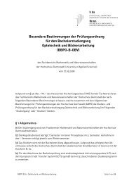
The following Table 1 reports some observations of “luminous phenomena” at the
sky.
observation
day day time space brightness
1 Monday morning east luminous
2 Monday evening west luminous
3 Tuesday morning east luminous
4 Tuesday evening west luminous
Table 1 : Observations of stars
For example, the observation labeled “1” states that at Monday morning in the east a
luminous phenomenon was observed.
We represent this table formally as a many-valued context and describe the background
theory of the meaning of the values by conceptual scales. Using nominal

scales as in [25] the derived context [25] has the concept lattice represented by the
line diagram in Figure 1.
luminous
east
morning
west
evening
Monday
Tuesday
1
2
3
4
Figure 1: A line diagram of the concept lattice of the nominally scaled manyvalued
context in Table 1.
Now, we give a short description of the main idea for the introduction of objects and
their life tracks. If we assume that the four observations of Table 1 are “caused” by a
single object, called “Venus”, then it seems to be clear to draw the “life track” of
Venus as in Figure 2.
luminous
east
morning
west
evening
Monday
Tuesday
1
2
3
4
Figure 2: The life track of Venus
But until now we did not represent any ordering in our time description. Therefore,
together with the introduction of an object we should represent formally that this
object may be observed differently in different observations. Hence, each observation
tells us something about the “actual object” observed during that observation. Therefore
we introduce four actual objects for Venus, called (v,0), (v,1), (v,2), (v,3) and
introduce a binary relation among the actual objects, usually a sequence of actual
objects, in our example: (v,0) → (v,1) → (v,2) → (v,3) .

We interpret the labels 0,1,2,3 in the actual objects as the “eigentime” (also called
“proper time” in physics) of the object Venus. The common letter “v” characterizes
the object Venus, an arrow of the time relation, for example (v,0) → (v,1), is interpreted
as “the change of (v,0) to (v,1)”. Therefore, this time relation seems to be a
suitable formal representation of the often used term “arrow of time” in physics
[11,12]. It also represents nicely the ideas of Kant [15] mentioned in section 1.2.
If we interpret the four observations of Table 1 as being caused by two stars, say
the “Morning Star” and the “Evening Star” then we would draw the “life tracks” of
them as in Figure 3.
luminous
east
morning
west
evening
Monday
Tuesday
1
2
3
4
Figure 3: The life tracks of Morning Star and Evening Star
The corresponding conceptual time system with actual objects and a time relation
(CTSOT) has the following data table:
actual objects day day time space brightness
(ms,0) Monday morning east luminous
(es,0) Monday evening west luminous
(ms,1) Tuesday morning east luminous
(es,1) Tuesday evening west luminous
Table 2: The data table of a conceptual time system with actual objects
Its time relation is given by : (ms,0) → (ms,1) , (es,0) → (es,1) .
In the following section we introduce the time dimension of a CTSOT.

3 Time Dimension and Life Tracks
After the demonstration of some examples we now need the formal definition of a
CTSOT to introduce the time dimension of a CTSOT.
3.1 Basic Definitions
We just recall the basic definitions and relate them to the given examples.
Definition: 'conceptual time system'
Let G be an arbitrary set (of time objects) and T := ((G, M, W, I T
), (S m
| m ∈ M)) and
C := ((G, E, V, I), (S e
| e ∈ E )) scaled many-valued contexts (on the same object set
G). Then the pair (T, C) is called a conceptual time system on G. T is called the time
part and C the event part of (T, C). The scales S m
and S e
of the time and event part
describe the chosen granularity strucure for the values in these many-valued contexts.
Example: Table 1 is the data table of a conceptual time system where G := {1,2,3,4},
the two columns labeled “day” and “day time” represent the many-valued context of
the time part, the two columns labeled “space” and “brightness” represent the manyvalued
context of the event part. The used nominal scales are described in [25].
Definition: 'conceptual time systems with actual objects and time relation'
Let P be a set (of 'persons', or 'objects', or 'particles') and G a set (of 'points of time')
and Π ⊆ P×G a set (of 'actual objects'). Let (T, C) be a conceptual time system on Π
and R ⊆ Π × Π. Then the tuple (P, G, Π, T, C, R) is called a conceptual time system
(on Π ⊆ P×G) with actual objects and a time relation R, shortly a CTSOT.
For each object p ∈ P the set p Π := {g ∈ G| (p,g) ∈ Π} is called the (eigen)time of p
in Π (which is the intent of p in the formal context (P, G, Π)). Then the set
R p
:= {(g,h) | ((p,g), (p,h)) ∈ R } is called the set of R-transitions of p and the relational
structure (p Π , R p
) is called the (eigen)time structure of p.
Example: Table 2 is the data table of a CTSOT where P := {ms,es} is the set of
Morning Star and Evening Star, G := {0, 1} the set of points of time. In this example
Π = P×G and R := {((ms,0), (ms,1)) , ((es,0), (es,1))}. The relational structure ({0,
1}, {(0,1)}) is the common eigentime structure of the Morning Star and the Evening
Star. The conceptual time system of this CTSOT is described in the previous example.
Definition: 'life track of an object'
Let (P, G, Π, T, C, R) be a CTSOT, and p ∈ P. Then for any mapping f: {p}×p Π →
X (into some set X) the set f = {((p,g),f(p,g))|g ∈ p Π } is called the f-life track (or f-
trajectory or f-life line) of p. The two most useful examples for such mappings are the
object mappings γ and γ C
of the derived contexts K T
⏐K C
and K C
of the conceptual
time system (T, C, R) on Π, each of them restricted to the set {p}×p Π of actual ob-

jects. They are called the life track of p in the situation space and the life track of p in
the state space respectively.
Example: The life tracks of “Morning Star” and “Evening Star” in the situation space
(where the time and the event part is represented) are shown in Figure 3 (where the
labels 1,2,3,4 clearly should be replaced by the actual objects (ms,0), (es,0), (ms,1),
(es,1)).
3.2 Dimensions
Definition: 'order dimension of an ordered set'
An ordered set (P, ≤) has order dimension dim(P, ≤) = n if and only if it can be order
embedded in a direct product of n chains and n is the smallest number for which this
is possible ([9], p. 236). As usual, a chain is an ordered set (M, ≤) such that for any
two elements a, b ∈ M a ≤ b or b ≤ a.
Clearly, the order dimension of the ordered set (R, ≤), the set of real numbers and
their usual ordering, equals 1 and the n-fold direct product of this ordered set, the
usual real n-dimensional space with the product order (R n , ≤) has order dimension n.
Definition: 'order dimension of a scaled many-valued context'
The order dimension of a scaled many-valued context ((G, M, W, I), (S m
| m ∈ M)) is
the order dimension of the concept lattice of its derived context.
Definition: 'scale dimension of a scaled many-valued context'
The scale dimension of a scaled many-valued context ((G, M, W, I), (S m
| m ∈ M)) is
the sum of the order dimensions of the concept lattices of the scales S m
(m ∈ M).
Since the concept lattice of the derived context of a scaled many-valued context can
be order embedded in the direct product of the concept lattices of the scales (see [9],
p. 77) we obtain:
Lemma 1:
The order dimension of a scaled many-valued context is less or equal to its scale
dimension.
Definition: 'time dimension of a conceptual time system'
Let (T, C) be a conceptual time system. The time dimension of (T, C) is the order
dimension of the time part T. Analogously, the (event or) space dimension of (T, C) is
the order dimension of the event part C.
Example: To demonstrate that these dimensions of a conceptual time system are a
useful and for practical purposes relevant notion we study a formal representation of
the following story:

A participant p of an international conference, let’s say the ICCS 2003, travels
on Sunday morning from Darmstadt to Dresden, arrives at Dresden in the
afternoon, visits the conference until Wednesday afternoon, then he has to
travel back to Darmstadt arriving there in the evening.
Figure 4 : Life tracks of a journey to Dresden: time scale dimension = 2
In Figure 4 we have drawn (in a simplified way) the life tracks of the participant p in
the state space, in the 2-dimensional time scale, and in the direct product of these two
lattices, namely the situation space. To sketch the precise construction we represent
the data table of the corresponding CTSOT with a single person p in Table 3:
R actual person day day time town
(p,0) Sunday morning Darmstadt
(p,1) Sunday afternoon Dresden
(p,2) Wednesday afternoon Dresden
(p,3) Wednesday evening Darmstadt
Table 3: The data table of the Dresden journey
The three arrows represent the time relation R on the set of actual persons. The two
attributes “day” and “day time” of the time part T and the attribute “town” of the
event part C are scaled by ordinal scales of order dimension one. Therefore, the scale
dimension of the time part T is two. Since the derived context of the time part of this
CTSOT has a chain as its concept lattice the time dimension equals one. Clearly, if
we would extend the CTSOT by a new actual object, say (p,3.0) which was at
Wednesday morning in Dresden and change the time relation to (p,0) → (p,1) →
(p,2) → (p,3.0) → (p,3) then the time dimension would be two. That demonstrates
why we are often interested only in the scale dimension.

3.3 The Unique-State Theorem
A very popular statement, namely that each system is in each point of time in exactly
one state can be made precise for CTSOTs and can be proven easily.
Definition:
Let (P, G, Π, T, C, R) be a CTSOT and (p,g) ∈ Π. We say that p is at time point g in
the situation s (or that the actual object (p,g) is in the situation s) iff s = γ((p,g)); (p,g)
is in the time state s iff s = γ T
((p,g)), and (p,g) is in the state s iff s = γ C
((p,g)).
Theorem: 'unique-state theorem'
Let (P, G, Π, T, C, R) be a CTSOT. Then each object p ∈ P is at each time point g of
its eigentime in exactly one situation, in exactly one time state and in exactly one
state.
Proof: Let (p,g) ∈ Π, then clearly γ((p,g)) is the only situation s such that p is at time
point g in the situation s. In the same way the rest of the theorem can be proved.
Remark: We do not know any formal theory where this popular theorem was stated or
even proved. It seems to be that some people use that statement as a kind of description
of a state.
It seems to be obvious that as a consequence of the unique-state theorem the eigentime
structure of an object looks like a (graph theoretic) chain, for example 0 → 1 →
2. That is not true as shown in the next section.
3.4 Branching Time and Branching Objects?
The following example demonstrates a CTSOT with a single object and a “branching”
time relation. It describes an “abstract letter”, that is a class of “identical” copies
of an original letter. As usual, we say that the abstract letter is sent from A to B iff a
copy of the original letter is sent from A to B.
Example: 'an abstract letter'
An abstract letter is sent on day 0 from place A to place B arriving there on day 1,
and on day 0 from A to the place C arriving there on day 2. Then the letter is sent on
day 1 from B to the place D and on day 2 from C to D either arriving on day 3.
Some of the information is represented in the following CTSOT with an ordinal scale
for the attribute “day” and a nominal scale for the “place”.

Table 4: A “branching” abstract letter
R actual objects day place
(letter,0) 0 A
(letter,1) 1 B
(letter,2) 2 C
(letter,3) 3 D
Clearly, this “branching” abstract letter can be described by its copies as in Table 5.
Table 5: Two copies as “simple” objects
R actual objects day place
(copy1,0) 0 A
(copy1,1) 1 B
(copy1,3) 3 D
(copy2,0) 0 A
(copy2,2) 2 C
(copy2,3) 3 D
Therefore, it is necessary to introduce a clear definition of “simple” objects:
Definition: 'simple objects'
An object p of a CTSOT is called simple iff the restriction of the time relation R on
the actual objects of p, i.e. R ∩ ({p}×p Π ) 2 , has a chain c p
:= ({p}×p Π , ≤ p
) as its reflexive
and transitive closure.
Let p be a simple object of a CTSOT and f: {p}×p Π → X a mapping into some set X.
Then the f-life track {((p,g), f(p,g)) | g ∈ p Π } of p can be ordered in a trivial way
isomorphically to c p
by the following definition of an order relation ≤ f
on f:
((p,g), f(p,g)) ≤ f
((p,h), f(p,h)) : ⇔ (p,g) ≤ p
(p,h).
Hence the ordered life-track (f, ≤ f
) of a simple object p is one-dimensional in the
sense that it is a chain (which is isomorphic to c p
). Note that f need not be injective.
4 Conclusion and Future Research
It is shown that Conceptual Time Systems with Actual Objects and a Time Relation
(CTSOT) allow for distinguishing clearly between the time dimension of a conceptual
time system and the order dimension of the chain c p
of a simple object of a CTSOT.
The shown existence of non-simple objects and their applicability to ideas like an
“abstract letter” open up interesting problems in the conceptual representation of
central notions in other branches of science like for example in computer science
where “information” and “object oriented programming” and its time-conceptual

foundations as developed by the second author in [29] now can be investigated from a
formal conceptual base. Clearly, also many fundamental problems in physics
[11,12,13] and Temporal Logic [7,19] will be studied using these methods.
5 References
1. Arbib, M.A.: Theory of Abstract Automata. Prentice Hall, Englewood Cliffs, N.J.,
1970.
2. Aristoteles: Philosophische Schriften in sechs Bänden. Felix Meiner Verlag Hamburg
1995.
3. Eilenberg, S.: Automata, Languages, and Machines. Vol. A. Academic Press 1974.
4. Einstein, A.: Zur Elektrodynamik bewegter Körper. Annalen der Physik 17 (1905):
891-921.
5. Einstein, A.: Über das Relativitätsprinzip und die aus demselben gezogenen Folgerungen.
In: Jahrbuch der Radioaktivität und Elektronik 4 (1907) : 411-462.
6. Einstein, A.: The collected papers of Albert Einstein. Vol. 2: The Swiss Years:
Writings, 1900-1909. Princeton University Press 1989.
7. Gabbay, D.M., I. Hodkinson, M. Reynolds: Temporal Logic – Mathematical
Foundations and Computational Aspects. Vol.1, Clarendon Press Oxford 1994.
8. Ganter, B., R. Wille: Conceptual Scaling. In: F.Roberts (ed.) Applications of combinatorics
and graph theory to the biological and social sciences,139-167. Springer
Verlag, New York, 1989.
9. Ganter, B., R. Wille: Formal Concept Analysis: mathematical foundations. (translated
from the German by Cornelia Franzke) Springer-Verlag, Berlin-Heidelberg
1999.
10.Gottwald, S. (ed.): Lexikon bedeutender Mathematiker. Bibliographisches Institut
1990.
11.Hawking, S.: A Brief History of Time: From the Big Bang to Black Holes. Bantam
Books, New York 1988.
12.Hawking, S.: Penrose, R.: The Nature of Space and Time. Princeton University
Press, 1996.
13.Isham, C.J.: Time and Modern Physics. In: Ridderbos, K. (ed.): Time. Cambridge
University Press 2002, 6-26.
14.Kalman, R.E., Falb, P.L., Arbib, M.A.: Topics in Mathematical System Theory.
McGraw-Hill Book Company, New York, 1969.
15.Kant, I.; Kritik der reinen Vernunft, in: Weischedel, W. (ed.): Immanuel Kant –
Werke in sechs Bänden. Band II, Insel Verlag, Wiesbaden 1956 (first edition
1781).
16.Lin, Y.: General Systems Theory: A Mathematical Approach. Kluwer Academic/
Plenum Publishers, New York, 1999.
17.Mesarovic, M.D., Y. Takahara: General Systems Theory: Mathematical Foundations.
Academic Press, London, 1975.
18.Pawlak, Z.: Rough Sets: Theoretical Aspects of Reasoning About Data. Kluwer
Academic Publishers, 1991.

19.van Benthem, J.: Temporal Logic. In: Gabbay, D.M., C.J. Hogger, J.A. Robinson:
Handbook of Logic in Artificial Intelligence and Logic Programming. Vol. 4,
Epistemic and Temporal Reasoning. Clarendon Press, Oxford, 1995, 241-350.
20.Wille, R.: Restructuring lattice theory: an approach based on hierarchies of concepts.
In: Ordered Sets (ed. I.Rival). Reidel, Dordrecht-Boston 1982, 445-470.
21.Wille, R.: Introduction to Formal Concept Analysis. In: G. Negrini (ed.): Modelli e
modellizzazione. Models and modelling. Consiglio Nazionale delle Ricerche, Instituto
di Studi sulli Ricerca e Documentatione Scientifica, Roma 1997, 39-51.
22.Wolff, K.E.: A first course in Formal Concept Analysis - How to understand line
diagrams. In: Faulbaum, F. (ed.): SoftStat ´93, Advances in Statistical Software 4,
Gustav Fischer Verlag, Stuttgart 1994, 429-438.
23.Wolff, K.E.: Concepts, States, and Systems. In: Dubois, D.M. (ed.): Computing
Anticipatory Systems. CASYS´99 - Third International Conference, Liège, Belgium,
1999, American Institute of Physics Conference Proceedings 517, 2000, pp.
83-97.
24.Wolff, K.E.: A Conceptual View of Knowledge Bases in Rough Set Theory. In:
Ziarko, W., Yao, Y. (eds.): Rough Sets and Current Trends in Computing. Second
International Conference, RSCTC 2000, Banff, Canada, October 16-19, 2000, Revised
Papers, 220-228.
25.Wolff, K.E.: Temporal Concept Analysis. In: E. Mephu Nguifo & al. (eds.): ICCS-
2001 International Workshop on Concept Lattices-Based Theory, Methods and
Tools for Knowledge Discovery in Databases, Stanford University, Palo Alto
(CA), 91-107.
26.Wolff, K.E.: Transitions in Conceptual Time Systems. In: D.M.Dubois (ed.):
Computing Anticipatory Systems CASYS'2001, American Institute of Physics
Conference Proceedings.
27.Wolff, K.E.: Interpretation of Automata in Temporal Concept Analysis. In: U.
Priss, D. Corbett, G. Angelova (eds.): Integration and Interfaces. Tenth International
Conference on Conceptual Structures. Lecture Notes in Artificial Intelligence.
Springer-Verlag 2002.
28.Concepts in Fuzzy Scaling Theory: Order and Granularity. 7 th European Congress
on Intelligent Techniques and Soft Computing, Aachen 1999. Fuzzy Sets and Systems
132 (2002) 63-75.
29.Yameogo, W.: Conceptual Knowledge Processing. Time Conceptual Foundations
of Programming. Master Thesis. Department of Computer Science at Darmstadt
University of Applied Sciences, 2003.
30.Zadeh, L.A.: The Concept of State in System Theory. In: M.D. Mesarovic: Views
on General Systems Theory. John Wiley & Sons, New York, 1964, 39-50.
31.Zadeh, L.A.; Fuzzy sets. Information and Control 8, 1965, 338 - 353.
32.Zadeh, L.A.; The concept of a linguistic variable and its application to approximate
reasoning. Part I: Inf. Science 8,199-249; Part II: Inf. Science 8, 301-357;
Part III: Inf. Science 9, 43-80, 1975.