Upper Hunter Valley Particle Characterization Study Final

CSIRO MARINE & ATMOSPHERIC RESEARCH 

Upper Hunter Valley Particle 

Characterization Study 

Final Report 

17 September 2013 

Mark Hibberd, Paul Selleck, Melita Keywood 

CSIRO Marine & Atmospheric Research 

David Cohen, Eduard Stelcer and Armand Atanacio 

Institute for Environmental Research, ANSTO 

Prepared for 

NSW Office of Environment and Heritage (Contact: Matt Riley) 

NSW Department of Health (Contact: Wayne Smith)

ISBN: 978‐1‐4863‐0170‐6 

Citation 

Hibberd MF, Selleck, PW, Keywood MD, Cohen DD, Stelcer E and Atanacio, AJ (2013). Upper Hunter Particle 

Characterisation Study. CSIRO, Australia. 

Contact addresses: 


Private Bag 1 

Aspendale, Vic 3195 

Australia 

Institute for Environmental Research, ANSTO 

Locked Bag 2001 

Kirrawee DC, NSW 2232 

Australia 

Copyright and disclaimer 

© 2013 CSIRO To the extent permitted by law, all rights are reserved and no part of this publication 

covered by copyright may be reproduced or copied in any form or by any means except with the written 

permission of CSIRO. 

Important disclaimer 

CSIRO advises that the information contained in this publication comprises general statements based on 

scientific research. The reader is advised and needs to be aware that such information may be incomplete 

or unable to be used in any specific situation. No reliance or actions must therefore be made on that 

information without seeking prior expert professional, scientific and technical advice. To the extent 

permitted by law, CSIRO (including its employees and consultants) excludes all liability to any person for 

any consequences, including but not limited to all losses, damages, costs, expenses and any other 

compensation, arising directly or indirectly from using this publication (in part or in whole) and any 

information or material contained in it. 

‐

Contents 

Executive Summary ........................................................................................................................................... iii 

Acknowledgments ............................................................................................................................................ vii 

1 Introduction .......................................................................................................................................... 1 

1.1 Aim of Study ................................................................................................................................ 1 

1.2 Project description ...................................................................................................................... 1 

2 Sampling methodology ......................................................................................................................... 3 

2.1 Measurement sites ..................................................................................................................... 3 

2.2 Sampling equipment ................................................................................................................... 4 

3 Analysis techniques ............................................................................................................................... 7 

3.1 Mass measurements ................................................................................................................... 7 

3.2 Ion beam analysis (IBA) techniques ............................................................................................ 7 

3.3 Ion chromatography ................................................................................................................... 7 

3.4 Organic carbon (OC) and Elemental carbon (EC) analysis .......................................................... 8 

3.5 Black carbon (BC) analysis .......................................................................................................... 9 

3.6 Positive matrix factorisation (PMF) ............................................................................................ 9 

3.7 Wind sector analysis ................................................................................................................... 9 

4 Monitoring results ............................................................................................................................... 11 

4.1 PM 2.5 time series ....................................................................................................................... 11 

4.2 Wind .......................................................................................................................................... 12 

4.3 Singleton PM 2.5 speciation ........................................................................................................ 14 

4.4 Muswellbrook PM 2.5 speciation ................................................................................................ 16 

4.5 Correlations............................................................................................................................... 17 

4.6 PM 2.5 mass closure .................................................................................................................... 18 

5 Data analysis by PMF .......................................................................................................................... 20 

5.1 Selection of species ................................................................................................................... 20 

5.2 PMF model diagnostics ............................................................................................................. 22 

6 Source apportionment ........................................................................................................................ 23 

6.1 Factor 1 – Woodsmoke ............................................................................................................. 24 

6.2 Factor 2 – Vehicle/Industry (Fe and BC) ................................................................................... 26 

6.3 Factor 3 – Secondary Sulfate .................................................................................................... 28 

6.4 Factor 4 – Biomass Smoke ........................................................................................................ 29 

6.5 Factor 5 – Industry Aged Sea Salt ............................................................................................. 32 

6.6 Factor 6 – Soil ............................................................................................................................ 33 

6.7 Factor 7 –Sea salt ...................................................................................................................... 35 

6.8 Factor 8 – Secondary Nitrate .................................................................................................... 36 

6.9 Seasonal variability ................................................................................................................... 37 

Upper Hunter Valley Particle Characterization Study. Final Report, 17 Sep 2013 | i

7 Discussion ............................................................................................................................................ 39 

7.1 Coal dust contributions ............................................................................................................. 40 

7.2 Power station contributions ..................................................................................................... 40 

8 Conclusions ......................................................................................................................................... 42 

References ........................................................................................................................................................ 44 

Appendix A Data quality: Sampling .............................................................................................................. 46 

Appendix B Data quality: Analysis ............................................................................................................... 48 

Appendix C Data Quality: PMF ..................................................................................................................... 54 

ii | Upper Hunter Valley Particle Characterization Study. Final Report, 17 Sep 2013

Executive Summary 

This study provides an analysis of the composition of PM 2.5 (particulate matter with a diameter of less than 

2.5 micrometres) in the two main population centres in the Upper Hunter, namely Muswellbrook and 

Singleton, during 2012.The finer PM 2.5 particles have been studied because they are of greatest concern 

owing to their impact on health. 

Samples were collected for 24 hours every third day and analysed for the components of PM 2.5 , specifically 

twenty elements, fourteen soluble ions, two anhydrous sugars (levoglucosan and mannosan) that are found 

in woodsmoke, organic carbon (OC), and black carbon (BC), as well as gravimetric mass. 

The chemical composition of all the samples from each site was analysed using a mathematical technique 

called Positive Matrix Factorisation (PMF), which is widely used in air pollution source apportionment 

studies. This identified eight factors (also called ‘fingerprints’) which represent the mix of components that 

tend to vary together in time. Further analysis, using information about known sources and knowledge of 

atmospheric chemistry as well as wind sector and seasonal analysis, was undertaken to identify the most 

likely source of emissions for each factor and hence the contribution that each source makes to the 

measured PM 2.5 concentrations. 

The veracity of the final results was confirmed by the good agreement between separate analyses using 

two different PMF techniques (EPA PMF 3.0 and PMF2 DOS). The differences between them provide an 

indication of the uncertainties in apportioning source contributions, which was typically 10% of each source 

contribution. The results for the whole year from the CSIRO PMF analysis are summarised in Table 1. At 

Singleton the dominant factors during the year were identified as: 

Factor 3 (Secondary Sulfate), 20 ± 2% 

Factor 5 (Industry Aged Sea Salt), 18 ± 3% 

Factor 2 (Vehicle/Industry), 17 ± 2% 

Factor 1 (Woodsmoke), 14 ± 2% 

Factor 6 (Soil), 12 ± 2%. 

At Muswellbrook the dominant factors were identified as: 

Factor 1 (Woodsmoke), 30 ± 3% 

Factor 3 (Secondary Sulfate), 17 ± 2% 

Factor 5 (Industry Aged Sea Salt), 13 ± 2% 

Factor 4 (Biomass Smoke), 12 ± 2% 

Factor 6 (Soil), 11 ± 1%. 

Table 1 lists the PMF factors, their names based on the dominant sources identified in their fingerprints, 

and the contribution of each factor to the total PM 2.5 concentrations in Singleton and Muswellbrook. 

The identification of most of the Factors is reasonably clear‐cut because of the use of either unique tracer 

species, e.g. levoglucosan for Factor 1 (Woodsmoke), or two or more species whose ratios are defined by a 

particular source, e.g. Si and Al in Factor 6 (Soil), Na + and Mg 2+ in Factor 7 (Sea Salt), and NH 4 + and SO 4 2‐ in 

Factor 3 (Secondary Sulfate). However in the case of Factor 2 (Vehicle/Industry) and Factor 4 (Biomass 

Smoke), the identification of the source is less definitive. 

Upper Hunter Valley Particle Characterization Study. Final Report, 17 Sep 2013 | iii

Factor 1 (Woodsmoke) dominates at both sites during the winter, while Factor 3 (Secondary Sulfate) and 

Factor 5 (Industry Aged Sea Salt) make higher contributions during summer months. The seasonal 

variations in the contributions from each factor are shown in Figure 1 and Figure 2. 

Table 1 Summary of the PMF factors (from the EPA PMF 3.0 analysis), main species, contributions of these factors at 

each site and potential sources 

Factor Main Species in Factor Contribution of the factor to 

total annual PM 2.5 mass at: 

Factor 1 

Woodsmoke 

Factor 2 

Vehicle/Industry 

Factor 3 

Secondary Sulfate 

Factor 4 

Biomass Smoke 

Factor 5 

Industry Aged Sea Salt 

Factor 6 

Soil 

Factor 7 

Sea Salt 

Factor 8 

Secondary Nitrate 

levoglucosan, mannosan, 

OC1 

BC, OC1, OC2, SO 4 2‐ Fe, 

Zn, Mn, Cu 

NH 4 + , SO 4 

2‐ 

OC2, OC3, OC4, K, SO 4 2‐ , 

Al, Si, Ti, BC 

Singleton Muswellbrook 

Potential Sources 

14 ± 2% 30± 3% Domestic woodheaters 

17 ± 2% 8 ± 1% Vehicles, industry 

20 ± 2% 17 ± 2% Local and regional 

sources of SO 2 such as 

power stations 

8 ± 2% 12 ± 2% Wildfires, hazard 

reduction burns 

Na + , Mg 2+ , SO 2‐ 4 and with 18 ± 3% 13 ± 2% Sea salt, local and 

almost no Cl ‐ regional sources of SO 2 

such as power stations 

Al, Si, Ca, Ti and Fe 12 ± 2% 11 ± 1% Soil dust, fugitive coal 

dust 

Na + , Cl ‐ , and Mg 2+ 8 ± 1% 3 ± 1% Sea salt 

NO 3 ‐ and includes some 

NH 4 + , Cl ‐ , Na + , OC 

3 ± 2% 6 ± 1% Motor vehicle NO 2 , 

power station NO 2 

Notes: Al – aluminium; BC – black carbon; Ca – calcium; Cl ‐ – chloride; Cu – copper; Fe – iron; K – potassium; Mg 2+ – 

magnesium; Mn – manganese; Na + – sodium; NH 4 + – ammonium; NO 3 ‐ – nitrate; OC1‐OC4 – fractions of organic 

carbon distinguished by the volatility of the organic compounds, OC1 is the most volatile, as organic aerosol ages its 

OC becomes less volatile; Si – silicon; SO 4 2‐ – sulfate; Ti – titanium; Zn – zinc. 

Figure 1 Annual and seasonal contributions of the PMF factors to PM 2.5 in Singleton 

iv | Upper Hunter Valley Particle Characterization Study. Final Report, 17 Sep 2013

Figure 2 Annual and seasonal contributions of the PMF factors to PM 2.5 in Muswellbrook 

Upper Hunter Valley Particle Characterization Study. Final Report, 17 Sep 2013 | v

vi | Upper Hunter Valley Particle Characterization Study. Final Report, 17 Sep 2013

Acknowledgments 

This is a CSIRO co‐investment project funded by 

NSW Office of Environment & Heritage 

NSW Department of Health 

CSIRO Climate & Atmosphere Theme 

We acknowledge the assistance provided by OEH staff in organising, setting up and running the sampling 

equipment – Chris Eiser, Melinda Hale, Scott Thompson, Matt Flack and John Kirkwood. 

We acknowledge the contributions of the ANSTO project team: Peter Drewer who assisted with the 

sampling program and the ANSTO accelerator staff involved in the IBA analyses. 

We acknowledge the contributions of the CSIRO project team: Kate Boast, Fabienne Reisen and Mahendra 

Buhjel for the analyses. 

Upper Hunter Valley Particle Characterization Study. Final Report, 17 Sep 2013 | vii

1 Introduction 

1.1 Aim of Study 

The objective of the Upper Hunter Valley Particle Characterization Study was to determine the major 

components and sources of particulate matter (as PM 2.5 – particles with a diameter of less than 

2.5 micrometres) in the two main population centres in the Upper Hunter Valley, namely Singleton and 

Muswellbrook (Figure 3, see also Figure 35). 

Figure 3 Overview of the Upper Hunter showing the locations of the measurement sites used in this study at 

Singleton and Muswellbrook (urban areas shaded pink) as well as the location of the two coal‐fired power stations. 

1.2 Project description 

This project collected PM 2.5 samples in the two main population centres in the Upper Hunter, namely 

Muswellbrook and Singleton during the full calendar year of 2012. Two different types of samplers were 

used to collect 24‐hour samples from midnight to midnight every third day. Two samplers were required 

since different chemical analyses require different filter media. One sampler collected particles on quartz 

fibre filters for the analysis of organic carbon, elemental carbon, soluble ions, and anhydrous sugars, while 

the second sampler collected particles on stretched Teflon filters for the analysis of elemental composition, 

soluble ions, black carbon and gravimetric mass. A range of analysis techniques was employed to determine 

the concentrations of these species. The chemical composition of all the samples from each site was then 

Upper Hunter Valley Particle Characterization Study. Final Report, 17 Sep 2013 | 1

analysed using Positive Matrix Factorisation to determine source fingerprints and the contribution that 

each source makes to the total PM 2.5 concentrations. This analysis provides: 

 

 

 

a description of the contributors to fine particles in the Upper Hunter 

an estimate of which sources are important and their relative contribution to fine particles in the 

Upper Hunter 

an indication of seasonal changes in the relative importance of the various sources to PM 2.5 in the 

Upper Hunter. 

2 | Upper Hunter Valley Particle Characterization Study. Final Report, 17 Sep 2013

2 Sampling methodology 

2.1 Measurement sites 

Figure 3 shows the location of the monitoring sites in Singleton and Muswellbrook in the Upper Hunter 

valley of NSW, Australia. The many open‐cut coal mines show up as white areas. There are two major 

power stations (Bayswater and Liddell) situated between the two towns with a total installed generating 

capacity of 5.6 GW. The axis of the valley is aligned approximately north‐west to south‐east with Singleton 

located about 70 km from the coast. 

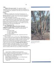
Figure 4 shows the location of the Singleton site with respect to rest of the town, the surrounding 

agricultural land and the nearest mine sites. Figure 6 shows a photograph of the monitoring station with 

the view towards the north. 

The equivalent information for the Muswellbrook site is given in Figure 5 and Figure 6, with latter showing 

the view towards the south‐east. 

Figure 4 Location maps for Singleton monitoring site (X) at 32.5575°S, 151.1769°E 

Figure 5 Location maps for Muswellbrook monitoring site (X) at 32.2717°S, 150.8858°E 


Figure 6 Monitoring stations at Singleton (left) and Muswellbrook (right), which are part of the Upper Hunter Air 

Quality Monitoring Network (UHAQMN) 

At both sites the equipment was located on the roof platforms of the NSW Office of Environment and 

Heritage (OEH) Upper Hunter Air Quality Monitoring Network (UHAQMN) sites. These sites include 

equipment to make routine measurements of PM 2.5 concentrations using a BAM (beta attenuation mass 

monitor) and PM 10 measurements using a TEOM (tapered element oscillating microbalance) as well as NO 2 

and SO 2 concentrations and meteorological measurements of temperature, relative humidity, wind speed 

and wind direction using an ultrasonic anemometer. 

2.2 Sampling equipment 

Two types of sampling equipment were used in this study that enabled the analysis of a wide range of 

constituents. These were: 

 

 

Ecotech HiVol 3000 high volume samplers with a PM 2.5 size selective inlet. These PM 2.5 samples 

were collected on quartz tissue filters and analysed by CSIRO. 

ANSTO ASP (Aerosol Sampling Program) PM 2.5 particulate Cyclone samplers with 25mm stretched 

Teflon filters. These samples were analysed by ANSTO and CSIRO. 

Both types of samplers were installed at each site on the roof‐top sampling platform about 4 m above the 

ground. 

Note that different filters were required for the various analyses. The method for determining OC (organic 

carbon) and EC (elemental carbon) involves combusting the sample, hence a filter substrate that includes 

organic material (such as Teflon) is not appropriate because it will have very high blank concentrations. 

Similarly the fibrous nature of the quartz filters means that their gravimetric mass is not stable, so that 

quartz filters cannot be used for the determination of gravimetric mass. The ultra thin stretched Teflon 

filters together with the low volume sampling are optimised for IBA techniques at ANSTO. Finally, quartz 

filters cannot be used for ion beam analysis (such as PIXE) because they are typically too thick and have 

high blank elemental concentrations. 

2.2.1 HIGH VOLUME SAMPLER 

An Ecotech 3000 high volume sampler with a PM 2.5 size‐selective inlet was used (Figure 7). The ambient 

flow rate through the inlet is 67.8 m 3 hr ‐1 . The flow rate is controlled with a mass flow controller, and the 

ambient temperature and pressure are monitored during sampling so that both the ambient volumetric 

and standard flow rates can be determined. The flow rate was audited and calibrated using a calibration 

orifice plate every 3‐6 months. Samples were collected on 250 mm x 200 mm quartz membrane filters (Pall‐ 

Gelman; prebaked at 600°C for 4 hours to minimize for adsorbed organic vapours). Samples were collected 


for 24 hours from midnight to midnight (Australian Eastern Standard time) on a 1‐day‐in‐3‐cycle. The filters 

were stored in sealed containers within a freezer before and after the sampling. 

One field blank sample was collected once per month at each site by placing a pre‐baked filter into the 

sample holder and running the sampler for 1 minute (total of 24 field blank samples). The field blank filters 

were then subject to the same filter handling and analysis procedures as the sample filters. In addition for 

the collection of 50% of the samples, two filters were placed in the filter holder in sequence (front filter and 

back filter) to correct for sampling artefacts on the OC and EC concentrations. Positive artefacts arise from 

the adsorption of volatile gases onto the filter material and negative artefacts arise from the degassing of 

semi‐volatile compounds from the collected aerosol on the front filter which may be then absorbed onto 

the back filter. 

The sample collection rate was 100% in that all samples were returned to CSIRO for analysis. 

Figure 7 CSIRO high volume sampler at Singleton with flow rate calibration being carried out 

2.2.2 ANSTO PM 2.5 ASP SAMPLER 

The ANSTO built ASP sampling unit is a PM 2.5 cyclone type sampler based on the US EPA IMPROVE system 

used across North America in their National Parks air monitoring program. The cyclone operates at a flow 

rate of 22 L min ‐1 using a mass flow controller which results in a PM 2.5 particle size cut‐off. The particles are 

collected on a 25mm diameter thin stretched Teflon filter masked to 17 mm diameter to increase sample 

thickness and improve deposit uniformity. The filters and the sampling regime are specifically designed for 

the ANSTO ion beam analysis (IBA) system described below. Samples were collected over the same time 

period and on the same days as the high volume sampler to enable comparison of data. 

The sample collection rate was 100% in that all samples were returned to ANSTO for analysis. 


Figure 8 ANSTO ASP sampler with cover open for filter changing 


3 Analysis techniques 

3.1 Mass measurements 

The mass of PM 2.5 on the 25 mm Teflon filters was determined gravimetrically. The filters were weighed 

before and after the sampling period to determine the particulate mass collected and then divided by the 

total volume of air that passed through the filter to obtain the PM 2.5 concentration. The weighing was 

performed under controlled conditions of 22 ± 2°C and 50 ±10% relative humidity. 

3.2 Ion beam analysis (IBA) techniques 

The 25 mm Teflon filters were analysed non‐destructively on the ANSTO STAR 2MV accelerator using 

nuclear IBA techniques. 

The simultaneous IBA techniques applied are: 

 

 

 

Proton induced X‐ray emission (PIXE) – for analysis of elements from aluminium to lead in 

concentrations from a few ng m ‐3 upwards, as described in Cohen (1993). 

Proton induced gamma‐ray emission (PIGE) – for analysis of light elements such as fluorine and 

sodium in concentrations above 100 ng m ‐3 , as described in Cohen (1998). 

Proton elastic scattering analysis (PESA) – for analysis of hydrogen at levels down to 20 ng m ‐3 , as 

described in Cohen (1996). 

A full description of these methods and how they are used can be found on the ANSTO web page at 

www.ansto.gov.au/environment/iba together with key publications describing other fine particle studies at 

ANSTO. 

The elements whose concentrations were determined are: 

 

 

 

 

 

 

 

 

 

 

Hydrogen (H) 

Sodium (Na) 

Aluminium (Al) 

Silicon (Si) 

Phosphorous (P) 

Sulfur (S) 

Chlorine (Cl) 

Potassium (K) 

Calcium (Ca) 

Titanium (Ti) 

 

 

 

 

 

 

 

 

 

 

Vanadium (V) 

Chromium (Cr) 

Manganese (Mn) 

Iron (Fe) 

Cobolt (Co) 

Nickel (Ni) 

Copper (Cu) 

Zinc (Zn) 

Bromine (Br) 

Lead (Pb) 

3.3 Ion chromatography 

A 6.25 cm 2 portion of each quartz filter was analysed for major water soluble ions by suppressed ion 

chromatography (IC) and for anhydrous sugars including levoglucosan by high‐performance anion‐exchange 

chromatography with pulsed amperometric detection (HPAEC‐PAD). The filter portions were extracted in 

10 ml of 18.2 mΩ de‐ionized water. The sample is then preserved using 1% chloroform. The ANSTO teflon 

filter was also analysed for water soluble ions by IC after IBA was carried out by ANSTO. The Teflon filter 

was first wetted with 100 µl of methanol, extracted in 5 ml of 18.2 mΩ de‐ionized water and then 

preserved with 1% chloroform. 


Anion and cation concentrations were determined with a Dionex ICS‐3000 reagent free ion chromatograph. 

Anions were separated using a Dionex AS17c analytical column (2 x 250 mm), an ASRS‐300 suppressor and 

a gradient eluent of 0.75 mM to 35 mM potassium hydroxide. Cations were separated using a Dionex CS12a 

column (2 x 250 mm), a CSRS‐300 suppressor and an isocratic eluent of 20 mM methanesulfonic acid. 

Anhydrous sugar concentrations were determined by HPAEC‐PAD with a Dionex ICS‐3000 chromatograph 

with electrochemical detection. The electrochemical detector utilizes disposable gold electrodes and is 

operated in the integrating (pulsed) amperometric mode using the carbohydrate (standard quad) 

waveform. Anhydrous sugars are separated using a Dionex CarboPac MA 1 analytical column (4 x 250mm) 

with a gradient eluent of 300 mM to 550 mM sodium hydroxide. 

The species whose concentrations were determined are: 

Chloride (Cl ‐ ) 

Nitrate (NO 3 ‐ ) 

Sulfate (SO 4 2‐ ) 

Oxalate (C 2 O 4 ‐ ) 

Formate (HCOO ‐ ) 

Acetate (CH 3 COO ‐ ) 

Phosphate (PO 4 3‐ ) 

Methanosulfonate (MSA ‐ ) 

Sodium (Na + ) 

Ammonium (NH 4 + ) 

Magnesium (Mg 2+ ) 

Calcium (Ca 2+) 

Potassium (K + ) 

Levoglucosan (C 6 H 10 O 5 , an anhydrous sugar ‐ 

woodsmoke tracer) 

Mannosan (C 6 H 10 O 5 , an anhydrous sugar ‐ 

woodsmoke tracer) 

3.4 Organic carbon (OC) and Elemental carbon (EC) analysis 

The carbon in PM 2.5 is analysed to obtain two separate components – organic carbon and elemental carbon 

– because different sources emit different types of carbon. Elemental carbon is principally emitted during 

the combustion of fossil fuels as small, sooty particles often with other chemicals attached to their surface. 

Organic carbon is the carbon in organic compounds in PM 2.5 . In practice this includes most compounds that 

contain carbon, excluding particles that are just elemental carbon. Sources of organic carbon include traffic 

and industrial combustion 

Elemental and organic carbon analysis was performed using a DRI Model 2001A Thermal‐Optical Carbon 

Analyzer following the IMPROVE‐A temperature protocol (Chow et al., 2007). Laser reflectance is used to 

correct for charring, since reflectance has been shown to be less sensitive to the composition and extent of 

primary organic carbon. Prior to analysis of filter samples, the sample is baked in an oven to 910C for 10 

minutes to remove residual carbon. System blank levels are then tested until < 0.20 g C cm ‐2 is reported 

(with repeat oven baking if necessary). Twice daily calibration checks are performed to monitor possible 

catalyst degeneration. The analyser is reported to effectively measure carbon concentrations between 0.05 

– 750 g C cm ‐2 , with uncertainties in OC and EC of 10%. 

The IMPROVE‐A carbon method measures four OC fractions at four non‐oxidizing heat ramps (OC1 at 

140C, OC2 at 280C, OC3 at 480C, OC4 at 580C) and three EC fractions at three oxidizing heat ramps 

(EC1 at 580C, EC2 at 740C, EC3 at 840C). The quartz filter sample is held at the target temperature until 

all carbon is desorbed at that fraction. During the non‐oxidizing heat ramps some of the OC can be 

pyrolyzed and will not desorb until the oxidized stages. The quantity of OC that was pyrolyzed (OCpyro) 

during the non‐oxidizing heat ramps is determined based on the time the reflectance of the filter rises back 

up to its initial value. Total OC is then calculated from the addition of all the OC fractions plus OCpyro. Total 

EC is calculated from the addition of all the EC fractions minus OCpyro. 

As discussed in Appendix A, analysis of the initial results showed that EC was overestimated, and for the 

results presented in this report did not include OCpyro in the OC fraction. 


3.5 Black carbon (BC) analysis 

ANSTO measured black carbon (BC) on their 25 mm Teflon filters using a light absorption technique called 

the Laser Integrated Plate Method (LIPM). Black carbon concentrations generally agree well with elemental 

carbon concentrations (USEPA 2012) but differences arise because the two techniques each measure 

different but related properties of the carbon. As discussed in Appendix A because of problems identified in 

the EC measurements, the BC results were used in the PMF analysis. 

For LIPM measurements, light from a HeNe laser (wavelength 633 nm) is diffused and collimated to give a 

uniform beam across the Teflon filter. The transmitted signal intensity is measured using a photodiode 

detector on each filter before and after exposure. The BC concentration is estimated from these two 

transmission measurements assuming a mass absorption coefficient value of 7 m² g ‐1 for carbon particles. 

Full details can be found in a publication by Taha et al. (2007). 

3.6 Positive matrix factorisation (PMF) 

Positive Matrix Factorisation (PMF) is a multivariate factor analysis tool that decomposes a matrix of 

speciated sample data into two matrices – factor contributions and factor profiles. These factors are then 

interpreted to determine what sources are represented by these factors. This is done using measured 

source profile information, wind direction analysis, and emissions inventories (Norris et al., 2008). The 

method is described in greater detail by Paatero (1997). 

PMF is widely used in air pollution studies for source apportionment, including in Australia (e.g. Chan et al., 

2008; Cohen et al., 2011; Cohen et al., 2012). The US EPA has developed a software package to implement 

this technique and EPA PMF 3.0 (Norris et al., 2008). Analysis was also undertaken by ANSTO using PMF2 

DOS and these results are reported in Appendix C 

In the main analysis for this study, the chemical composition data of all the samples from each site was 

analysed using the EPA PMF software. This identified a number of factors. Each factor has a ‘fingerprint’ 

which represent a mix of components that generally occur together in the data. To understand what this 

means, consider a simplified example of fine particles of sea salt in the air formed from sea spray. The ratio 

of the concentrations of the main elements in sea water is well known – the ratio of [Na:Cl:Mg:Ca] is equal 

to [1:1.8:0.12:0.04]. Thus on days when there are fine sea salt particles in the PM 2.5 , the chemical analysis 

of the filters will show these elements occurring together in the above proportions. On some days, the 

concentrations will all be higher and on other days lower but the proportions will stay the same. It is this 

principal that underlies PMF. In practice, there are many potential sources of PM 2.5 but PMF does not 

require or use any a priori information about the chemical composition of possible PM 2.5 sources. Rather it 

uses a mathematical technique to identify the factors. Indeed an advantage of the PMF over other source 

apportionment techniques is that it is able to identify the presence of particles which are not directly 

emitted as particles (primary particles) but form by chemical reactions in the atmosphere and gas‐toparticle 

conversions (secondary particles). 

Once the factors are obtained, further analysis is undertaken to identify the sources in each factor. This 

uses information about known sources and other knowledge of atmospheric chemistry as well as wind 

sector and seasonal analysis to identify the most likely source of emissions for each factor and hence the 

contribution that each source makes to the total PM 2.5 concentrations. In many cases, there is a single 

dominant source in a factor and this has been used to name the factors in Section 6. However, if sources 

are co‐located or otherwise correlated, they can appear together in a single factor or across several factors. 

This is discussed in Section 6. 

3.7 Wind sector analysis 

To determine the directions from the sampling site which are likely to include the locations of the sources, 

the conditional probability function (CPF) technique was used. This couples the source contribution 


estimates from PMF with the wind directions measured at the sampling site (e.g. Kim and Hopke, 2004). 

The CPF estimates the probability that a given source contribution from a given wind direction will exceed a 

pre‐determined criterion. It is defined as 

CPF = m Δθ /n Δθ 

where m Δθ is the number of occurrences from wind sector Δθ that exceed the criterion and n Δθ is the total 

number of data from the same wind sector. In this study, the optimum value of the size of the wind sector 

Δθ was found to be 20°. Wind speeds below 0.5 m s ‐1 were excluded from the analysis as these were 

considered to represent calm conditions. 

Daily fractional mass contribution from each source was used rather than the absolute source contribution. 

The criterion was set as the upper 25 th percentile of the fractional contribution from each source. The same 

daily fraction was assigned to each hour of a given day to match the hourly wind data. Although it might 

seem more appropriate to match the (24‐hour average) PM 2.5 data with the corresponding 24‐hour average 

wind direction, the loss of information in averaging the wind directions produces poorer results from the 

CPF analysis than using the method outlined above. 


4 Monitoring results 

4.1 PM 2.5 time series 

Figure 9 shows the time series of 24‐hour average PM 2.5 concentrations measured at Singleton by the OEH 

Beta Attenuation Mass (BAM) monitor for 2012. The red symbols highlight the days when 1‐in‐3‐day 

sampling was carried out by CSIRO and ANSTO for the current study. It shows that these are representative 

of the full period, including days with both high and low PM 2.5 concentrations. The equivalent time series 

for Muswellbrook is given in Figure 10. 

Figure 9 Time series of 24‐hour average PM 2.5 concentrations measured by the OEH BAM (Beta Attenuation Mass) 

monitor at Singleton. The red symbols show the days when sampling for the current study was carried out. 

Figure 10 Time series as in previous figure but for Muswellbrook. 

By plotting the time series as running averages in Figure 11, it is easier to compare the PM 2.5 levels at the 

two sites and identify the elevated levels during the cooler months from May to October. 


Figure 11. Running averages of PM 2.5 to show the seasonal trends more clearly with elevated levels from May to 

October at both sites. 

Comparison in Figure 12 between the OEH PM 2.5 results and the gravimetric mass determination of PM 2.5 

from the ANSTO sampler shows that apart from a few outliers, the gravimetric mass is on average close to 

but about 16 – 18% lower than the BAM measurement – probably due to slight differences in the 

measurement techniques – but the agreement is considered to be good. 

Figure 12 Comparison of PM 2.5 measured on ANSTO filters and by OEH BAM instrument. 

4.2 Wind 

Both sites include wind direction and wind speed measurements as part of the routine measurements by 

OEH. The winds are generally aligned along the valley on a north‐west to south‐east axis. The 2012 seasonal 

wind roses for Singleton are shown in Figure 13 and for Muswellbrook in Figure 14. Summer winds are 

almost all from the south‐east whereas in winter most of the winds are from the north‐west, particularly in 

Singleton. The other seasons include a mix of these directions with a very infrequent north‐easterlies or 

south‐westerlies. The winds speeds measured at Singleton are higher because of its more exposed location. 


Figure 13. Seasonal wind roses for 2012 at the Singleton sampling site from 1‐hour average OEH data 

Figure 14. Seasonal wind roses for 2012 at the Muswellbrook sampling site from 1‐hour average OEH data 


4.3 Singleton PM 2.5 speciation 

Table 2 lists the species measured in the Singleton samples with their median concentration, minimum 

detection limit (MDL) and uncertainty. The table shows that OC (sum of OC1, OC2, OC3 and OC4) is the 

dominant component (OC includes the contributions from levoglucosan, mannosan and oxalate which are 

also resolved separately). The next most important species are black carbon/elemental carbon and sulfate. 

Table 2 Median concentrations for species measured at Singleton using either ion chromatography(IC), ion beam 

analysis (IBA), LIPM (laser integrated plate method (LIPM), or thermal‐optical carbon analyser (TA) 

Species 

Median 

Conc. 

MDL 

% of 

values 

Figure 15. Time series of selected constituents of the Singleton samples during 2012 


4.4 Muswellbrook PM 2.5 speciation 

Table 3 lists some of the properties of the species measured in the Muswellbrook samples. In most case the 

median concentrations are very similar to those in Singleton. The table shows that as in Singleton, the 

dominant component is organic carbon but its concentration is about 30% higher than in Singleton. The 

next most important species are black carbon/elemental carbon and sulfate, followed by levoglucosan 

which is 70% higher than in Singleton. 

Table 3. Median concentrations for species measured at Muswellbrook using either ion chromatography(IC), ion 

beam analysis (IBA), LIPM (laser integrated plate method (LIPM), or thermal‐optical carbon analyser (TA) 

Species 

Median 

Conc. 

MDL 

% of 

values 

Figure 16 Time series of selected constituents of the Muswellbrook samples during 2012 

4.5 Correlations 

Figure 17 displays the linear relationships between a number of key species that indicate the sources of 

these species. The Na + versus Mg 2+ shows that at both sites the slope of the lines is close to that of the ratio 


[Na + /Mg 2+ ] found in sea salt; the Si versus Al plot shows the slope at both sites is similar to the [Si/Al] ratio 

observed in crustal material. The linear relationships between nssSO 4 2‐ versus NH 4 + and levoglucosan versus 

OC1 indicate these species are related in their sources. 

1800 

4500 

1600 

4000 

Na + (ng m ‐3 ) 

1400 

1200 

1000 

800 

600 

y = 8.75x ‐ 23.90 

R² = 0.98 

y = 8.42x ‐ 13.96 

R² = 0.99 

nssSO 4 

2‐ 

(ng m ‐3 ) 

3500 

3000 

2500 

2000 

1500 

y = 3.18x + 204.11 

R² = 0.90 

y = 2.92x + 178.39 

R² = 0.80 

400 

200 

Muswellbrook 

Singleton 

Linear (Muswellbrook) 

Linear (Singleton) 

1000 

500 

Muswellbrook 

Singleton 



0 

0 20 40 60 80 100 120 140 160 180 200 

Mg 2+ (ng m ‐3 ) 

0 

0 200 400 600 800 1000 1200 1400 

NH 4 

+ 

(ng m ‐3 ) 

1200 

4000 

Si (ng m ‐3 ) 

1000 

800 

600 

400 

200 

y = 2.96x + 16.51 

R² = 0.95 

y = 2.96x + 15.70 

R² = 0.99 

Muswellbrook 

Singleton 



Levoglucosan (ng m ‐3 ) 

3500 

3000 

2500 

2000 

1500 

1000 

500 

y = 0.49x + 161.23 

R² = 0.79 

y = 0.79x + 143.90 

R² = 0.95 

Muswellbrook 

Singleton 



0 

0 50 100 150 200 250 300 350 

Al (ng m ‐3 ) 

0 

0 500 1000 1500 2000 2500 3000 3500 

OC1(ng m ‐3 ) 

Figure 17 Scatter plots showing linear relationships between key species which provide an indication of the sources 

of the species. 

4.6 PM 2.5 mass closure 

Figure 18 compares the PM 2.5 from the gravimetric measurement on the 25 mm Teflon filter against the 

sum of the species concentrations (with appropriate oxygen added) measured on the 25 mm Teflon filter 

and the OC fractions measured on the quartz filters. Although the average shows good agreement, there is 

considerable scatter. This arises from uncertainty in conversion of the measurement of organic carbon to 

organic mass. Russell (2003) reported conversion factors of 1.2 to 1.6 depending on the number of 

functional groups in the organic compounds. We used a value of 1.2 to match the average, but the large 

scatter remains unexplained. 

Figure 19 compares the PM 2.5 gravimetric measurement against the ANSTO reconstructed mass (RCM), 

where this is computed using the method reported by Malm, Sisler et al. (1994) as 

RCM = Salt + Ammonium Sulfate + Soil + Smoke + Organics + BC 

where: 

Salt = 2.54 [Na] 

Ammonium sulfate = 4.125 [S] 

Soil = 2.20 [Al] + 2.49 [Si] + 1.63 [Ca] + 1.94 [Ti] + 2.42 [Fe] 

Smoke = [K] – 0.6 [Fe] 

Organics = 11 [H] – 0.25 [S] assuming the average organic material is 9% hydrogen. 


The RCM is smaller than the gravimetric mass (by about 25%) because it does not include nitrates or water 

vapour. This proportion is typical for other ANSTO studies (e.g. (Cohen, Crawford et al. 2010)). 

Figure 18 Comparison between the sum of the masses of the constituents of PM 2.5 with the gravimetric mass 

measurements on the ANSTO PM 2.5 filters. The solid line is 1:1 correspondence, the dashed lines are ± 3 µg m ‐3 . 

Figure 19 Comparison between the sum of the reconstructed mass from the ANSTO IBA constituents of PM 2.5 with 

the gravimetric mass measurements on the ANSTO PM 2.5 Teflon filters 


5 Data analysis by PMF 

5.1 Selection of species 

The selection of species for inclusion in PMF analysis requires some discussion. The analytical methods used 

for the analysis of samples in this project have produced data sets for 46 species. In a number of cases 

different methods have measured the same or similar species (e.g. SO 4 

2‐ 

by IC and S by PIXE, EC by thermal 

desorption and BC by integrated plate method). In these cases one of these species has been selected for 

PMF. This has resulted in the removal of H, Na, S, Cl measured by PIXE, EC measured by thermal desorption 

and K + and Ca 2+ measured by IC (Table 4). 

Species Excluded 

H by PIXE 

Na by PIXE 

S by PIXE 

Cl by PIXE 

EC by thermal desorption 

K + by IC 

Ca 2+ by IC 

Cr, Co by PIXE, NO 2 ‐ , Br ‐ by IC 

P, V, Ni, by PIXE 

Table 4 Species excluded from the PMF analysis 

Reason 

Duplicate, so used OC1, OC2, OC3 and OC4 by thermal desorption 

Duplicate, so used Na + by IC 

Duplicate, so used SO 4 2‐ by IC 

Duplicate, so used Cl ‐ by IC 

EC data quality poor (see Appendix A), so replaced by BC 

Duplicate, so used K by PIXE 

Duplicate, so replaced by Ca by PIXE 

> 95% of data below MDL 

> 75% of data below MDL and poor fit 

MSA, F, acetate, formate by IC PMF model fit poor (r 2 < 0.6) 

In a number of cases a large proportion of the concentrations were below the MDL. The EPA PMF 3 Users 

Manual (Norris et al., 2008) recommends the exclusion of species if more than 95% of samples have 

concentrations less than the MDL. In addition species with more than 75% of samples less than the MDL 

were examined closely and their inclusion was dependent on how well the modelled time series fit the 

observational data. In other PMF analyses all species have been used in PMF regardless of whether they are 

consistently below the MDL (Cohen et al., 2012) or data below MDL concentrations are replaced with 

values of half the MDL (Poirot et al., 2001). The species removed from the PMF analysis due to the MDL 

criteria adopted for this work were P, V, Cr, Co, Ni, and Br (Table 4). 

We also used the criteria of the signal‐to‐noise (S/N) ratios to assign an uncertainty weighting to the 

species. Variables were initially defined to be good, weak or bad depending on their S/N ratio. Species with 

S/N ratios less than 0.2 were excluded (although all data had S/N ratios > 0.2). Species with S/N ratios 

between 0.2 and 2 were considered weak variables and by flagging them as such their estimated 

uncertainties were increased by a factor of 3 to reduce their weight in the solution. We also set the mass 

variable to weak assigning it as a totalising variable. 

Finally we evaluated the ability of PMF to model each species. PMF was unable to model MSA, F, acetate, 

formate so these species were removed from the PMF analysis. 

Table 5 and Table 6 list the strength of the various species used in the PMF analysis at Singleton and 

Muswellbrook respectively. There were a total of 123 samples from each site, each with 25 species 

included in the PMF analysis. 


Species 

PMF 

Categorization 

Table 5 Species included in PMF analysis at Singleton. 

S/N 

Median 

Concentration 

MDL 

% of values 

Table 6 Species included in PMF analysis at Muswellbrook. 

Species 

PMF 

Categorization 

S/N 

Median 

Concentration 

MDL 

% of values 

6 Source apportionment 

Eight factors were identified in the PMF analysis at each site. These are summarised in Figure 20 which 

shows the average portion of PM 2.5 explained by each factor at each site over the 2012 period. These 

factors are discussed in detail in the following sections. Figure 21 shows that the PMF solution is able to 

resolve close to 100% of the mass weighed on the 25 mm Teflon filters. 

Figure 20 Average portion of PM 2.5 mass explained by each factor in the PMF solution. 

Figure 21 Gravimetric PM 2.5 mass measured on the 25 mm Teflon filter versus mass determined by the EPA PMF 

solution. 

Each of the factors is characterised by a chemical ‘fingerprint’ which is a unique pattern of chemical species 

and their concentrations. Before considering each factor in turn, we describe here the interpretation of the 

three types of figures presented for each factor – the fingerprints, the time series and the CPF plots – using 

the figures for Factor 1 in Section 6.1. 


Interpretation of the fingerprints, time series and CPF plots 

Figure 22 shows an example of the ‘fingerprint’ of the factor, so called because it shows a unique pattern of 

species concentrations. The fingerprint shows the relative amounts of the various species in the factor. It 

does this in two ways. Firstly, the vertical blue bars show the species concentrations, e.g. in Factor 1 at 

Singleton, the levoglucosan concentration is 210 ng m ‐3 and the mass (second bar from the right) is 

920 ng/m 3 = 0.92 µg m ‐3 . Secondly, the dark red squares show the percentage of the species that occurs in 

the factor, e.g. Factor 1 at Singleton includes 86% of the levoglucosan measured in the samples and 14% of 

the mass. Both of these pieces of information (concentrations and percentages) are shown because both 

are important in analysing and interpreting the factors. 

Figure 23 shows how the contribution of the factor to total PM 2.5 varies during the year. Factor 1 only 

makes a significant contribution from May to August with almost no contribution from November to 

March. The figure shows that in Singleton there are some days in winter when up to 60% of the PM 2.5 is in 

this factor. These time series provide additional evidence that is used in deciding on the source of the 

emissions. For example, the cooler weather from May to August corresponds to the period when domestic 

woodheaters are used, and this agrees with the fingerprint analysis indicating woodsmoke. Smoke is also 

produced by bushfires and hazard reduction burns, but the time series of these in Figure 34 is quite 

different from the time series for Factor 1, indicating that bushfires and hazard reduction burns are not the 

sources of the woodsmoke in Factor 1 from May to August. 

Figure 24 shows the wind sector plot from the conditional probability function (CPF) analysis described in 

Section 3.7. In simple terms, the distance of the yellow line from the central yellow dot shows the 

percentage of time that sources in that wind direction contribute to the factor. Because of limitations of 

the analysis discussed in Section 3.7, attention should focus on the gross features and not the fine detail. 

Thus Figure 24 for Singleton shows roughly similar contributions from most wind directions except southeasterly, 

which indicates a disperse local source, which is consistent with what is known about this factor 

from Figure 23 and Figure 24. 

The differences between the gross features in the CPF plots for the various factors can be seen by 

comparing Figure 24 with the CPF figure for Factor 7 (Figure 44), which shows the strongest lobe for southeasterlies, 

i.e. for winds from the coast moving inland along the Hunter Valley. This is consistent with the 

sea salt source for this factor. 

6.1 Factor 1 – Woodsmoke 

The first factor (Factor 1) identified as the woodsmoke factor makes up 30% of the PM 2.5 mass at 

Muswellbrook and 14% of the mass at Singleton. It is characterised by high levels of levoglucosan, 

mannosan and organic carbon (OC1) (Figure 22). Levoglucosan and mannosan are unique tracers for the 

combustion of cellulose found in trees and plants (Iinuma et al, 2007). The ratio of levoglucosan to 

mannosan is an indication of the type of wood combusted. The correlation between levoglucosan and 

mannosan in the samples was extremely high (r 2 = 0.99) and the ratio of 36 is close to the value for 

eucalyptus of 34.9 ± 1.9 measured by Goncalves et al. (2010). 

Levoglucosan shows a clear linear relationship with OC1 (Figure 17). OC1 is the most volatile OC fraction 

measured by the IMPROVE‐A method (since it is the lowest temperature fraction). Generally as organic 

aerosol ages the organic compounds present become less volatile. Thus the good correlation between OC1 

and levoglucosan indicates the smoke is fairly fresh, as we would expect considering the proximity of the 

sampling sites to houses. 

This factor accounts for 30% of the annual average organic carbon (sum of OC1, OC2, OC3 and OC4) in 

Muswellbrook and 8% in Singleton. It also includes 22% of the BC in Muswellbrook and 4% in Singleton. 

The time series (Figure 23) show that the factor is only present during the cooler months of the year with 

significant contributions from May to August in both towns. In Muswellbrook it contributes up to twothirds 

of the PM 2.5 during the middle of winter and in Singleton up to one‐third. The CPF plots (Figure 24) 

show the direction of the sources being the urban areas with good consistency between the directions of 


the CPF lobes and the urban lobes except for south‐easterly winds. The Muswellbrook site is closer to 

houses (Figure 5) than the Singleton site (Figure 4), where the closest houses are to the south. 

This is similar to the Smoke factor identified by Cohen et al. (2012) in an analysis of 10 years of data from 

the Sydney Basin (2001 to 2011 at Richmond). In the absence of the unique woodsmoke tracer 

levoglucosan the species H, K and BC were used as the indicators. This factor grouped smoke from 

woodheaters and bushfire smoke together. At Richmond this factor contributed 37% on average to the 

PM 2.5 loading. A strong seasonal cycle was observed with maximum contributions occurring during winter. 

Singleton Factor 1 

Muswellbrook Factor 1 

1000 

concentration 

% of species 

100 

90 

1000 

concentration 

% of species 

100 

90 

concentration (ng m ‐3 ) 

100 

10 

1 

80 

70 

60 

50 

40 

30 

% of species 

concentration (ng m ‐3 ) 

100 

10 

1 

80 

70 

60 

50 

40 

30 

% of species 

0.1 

20 

10 

0.1 

20 

10 

0.01 

0 

0.01 

0 

Figure 22 Fingerprint of Factor 1 (Woodsmoke) at Singleton (left) and Muswellbrook (right) 

Figure 23 Time series of percentage that Factor 1 (Woodsmoke) contributes to PM 2.5 in Singleton and 

Muswellbrook; only contributes significantly during the cooler months May‐August. 

Figure 24 CPF plot of Factor 1 (Woodsmoke) at Singleton (left) and Muswellbrook (right). At both sites highest 

Woodsmoke source contributions at Singleton (left) were associated with winds from the north and south, while at 

Muswellbrook they were associated with winds from the southwest. 

This factor includes 42% of the lead detected in the samples at Muswellbrook and 31% at Singleton, and 

the time series for lead (bottom right panel of Figure 15 and Figure 16) are most similar to those for the 


levoglucosan and mannosan. It should be noted that the maximum 24‐hour average lead concentrations 

were extremely low – 9.5 ng m ‐3 in Singleton and 20.1 ng m ‐3 in Muswellbrook – compared to the NEPM 

(National Environmental Protection Measure) of 500 ng m ‐3 for the annual average lead concentration. It is 

postulated that the lead originates from the burning of small amounts of painted wood in domestic wood 

heaters, in spite of advice to the contrary by NSW EPA (1999). 

Only a very small amount of lead needs to be released by burning to produce the observed low 

concentrations. For example 1 g of lead released into and thoroughly mixed over an area 1 km x 1 km and 

to a depth of 100 m would produce an average concentration of 10 ng m ‐3 . If the volume of air were 

smaller, then a smaller amount of lead would be needed to reach 10 ng m ‐3 , and vice versa. Although 

modern paint is restricted to a maximum of 0.1% lead, prior to 1992 the limit was 1%, and prior to 1965 it 

could be up to 50% lead. Based on a typical paint coverage rate of 10 m 2 litre ‐1 , a 20 cm 2 piece of fifty year 

old painted wood could release about 1 g lead when burnt. 

6.2 Factor 2 – Vehicle/Industry (Fe and BC) 

Factor 2 makes up 8% of the PM 2.5 mass at Muswellbrook and 16% of the PM 2.5 mass at Singleton. This 

factor explains most of the variation in Fe at both sites (44% of Fe at Singleton and 55% at Muswellbrook) 

and explains 21% of BC at Muswellbrook and 58% of BC at Singleton. This factor also explains significant 

fractions of Cu, Mn and Zn in the samples (Figure 25). OC is also present. 

We have named this a Vehicle/Industry factor as the species present are found in both of these sources. 

The vehicle component could include direct vehicle emissions from the combustion of petrol and diesel, as 

well as emissions from brakes and tyre wear or resuspension of paved road dust. We discount the latter 

since the factor would be dominated by Si and Al if resuspension of roadside dust was the main contributor 

to the vehicle factor. Vehicle use in coal mining could contribute to this factor. 

The profile of species presented by Chow et al. (2004) for vehicle emission composite samples collected 

during the Big Bend Regional Aerosol Visibility and Observational Study is similar to the profiles of the 

species that make up most of the mass of the Factor 2 at both Singleton and Muswellbrook (Table 7). 

The wear of motor vehicle engines results in the emission of Fe, the wear of brakes in the emissions of Cu 

and tyres in the emission of Zn (Sternbeck et al., 2002). Thus the Fe and Zn present in this factor may be 

due to these processes. Calcium is used as in lubricating oil for diesel vehicles (Cheung et al., 2010). 

Manganese may be indicative of the fuel additive methylcyclopentadienyl manganese tricarbonyl (MMT), 

which during combustion releases inorganic Mn species (Joly et al. 2011). MMT has been used as a fuel 

additive in Australia since 2000 (NICNAS 2003). 

This factor could also be similar to an Auto factor identified by Cohen et al. (2011) based on 10 years (1999 

to 2009) of data at Liverpool in NSW. The dominant species were H, BC and Fe. Factor7‐Auto identified by 

Cohen et al. (2012), based on 10 years (2001 to 2011) of data at Richmond in NSW was dominated by H, BC 

and trace elements associated with motor vehicles such as Zn from tyre wear, P and Ca from engine oils 

and small amounts of Pb and Br associated with historic leaded petrol use. The contribution to the total 

mass from this fingerprint was also consistent with the motor vehicle use in the vicinity of the Richmond 

site (11%). Note that the Auto factor identified by Cohen et al. (2011) does not include Fe. 

Table 7 Dominant species in motor vehicle factors 

Location Species Reference 

Big Bend Regional Aerosol 

Visibility and Observational 

Study Vehicle composite 

Each > 10% OC1, OC2, OC3, OC, EC1, EC2, EC 

Each > 1% S, OC4 

Chow et al., 2004 

Richmond, Sydney (2001‐2011) H, BC, Zn, P, Ca Cohen et al., 2012 

Liverpool Sydney (1999 ‐2009) BC, Fe and H Cohen et al., 2011 


This factor could be similar to the Industry factor identified by Cohen et al. (2012) at Richmond where BC, 

Fe and Zn were used as the indicators and the likely industries were metal smelting or processing. At 

Richmond this factor only contributed 2% on average to the PM 2.5 loading consistent with it being a 

suburban site. 

In another source apportionment study, this time in Hanoi, Cohen et al. (2010) identified a factor 

dominated with BC, Fe and H and significant V and Ni tracers as an iron smelting source, which was 

supported by the presence of several such smelting operations within 24 km of the sampling site probably 

contributing to this source. However in the Upper Hunter Valley, Fe smelting is not carried out. 

The CPF plots (Figure 27) for this factor suggest that highest contributions from this source occurs with 

winds from the north and northwest at Singleton i.e. in the direction of the coal mines and most sectors at 

Muswellbrook but with significant contributions from a range of directions it probably includes local 

sources. It is interesting to note that the Singleton site is located closer to the mines than the 

Muswellbrook site and this factor makes a greater contribution to PM 2.5 at Singleton. 



concentration 

% of species 

concentration 

% of species 

1000 

100 

90 

1000 

100 

90 

concentration (ng m‐3) 

100 

10 

1 

0.1 

80 

70 

60 

50 

40 

30 

20 

10 

% of species 


100 

10 

1 

0.1 

80 

70 

60 

50 

40 

30 

20 

10 

% of species 

0.01 

0 

0.01 

0 

Figure 25 Fingerprint of Factor 2 (Vehicle/Industry) at Singleton (left) and Muswellbrook (right) 

Figure 26 Time series of percentage that Factor 2 (Vehicle/Industry) contributes to PM 2.5 in Singleton and 

Muswellbrook; weak seasonal variation but different at the two sites. 


Figure 27 CPF plot of Factor 2 (Vehicle/Industry) at Singleton (left) and Muswellbrook (right). The highest 

Vehicle/Industry contributions at Singleton (left) were associated with winds from the north and west i.e. in the 

direction of the coal mines and most sectors at Muswellbrook (right) but there are contributions from most other 

wind directions indicating local sources. 

6.3 Factor 3 – Secondary Sulfate 

Factor 3 contributes 17% to the PM 2.5 mass at Muswellbrook and 20% at Singleton. The factor is dominated 

by secondary ammonium sulfate with the factor accounting to 60% of the sulfate and 85% of the 

ammonium in the samples. 

Ammonium and sulfate occur in atmospheric particles as a result of photochemical reactions in the 

atmosphere. Gaseous sulfur dioxide (SO 2 ) is emitted to the atmosphere during combustion of fossil fuels 

(e.g. in power stations or motor vehicles) and in the presence sunlight will oxidise to form sulfuric acid 

(H 2 SO 4 ), which is a strong acid. The seasonal cycle displayed by the contribution of this factor to PM 2.5 mass 

in Figure 29 of higher contributions during the summer months represents the greater time for 

photochemical reactions to occur during the summer months. The only significant gaseous base in the 

atmosphere is ammonia which is globally derived from biological production, such livestock wastes and 

fertiliser. It plays an important role in neutralising acids in the atmosphere, hence readily neutralises the 

sulfuric acid to produce ammonium sulfate aerosol. 

The CPF plots (Figure 30) both have lobes to the north and south. This does not correspond to the major 

source of SO 2 in the region (the power stations) but reflects the fact that the chemical reactions to form the 

(NH 4 ) 2 SO 4 take time to occur. 

This is similar to Secondary Sulfate (2ndryS) identified by Cohen et al. (2012) at Richmond, although in that 

data set H was used as a surrogate for NH 4 + . At Richmond this factor contributed 27% on average to the 

PM 2.5 loading. A strong seasonal cycle was observed with maximum contributions occurring during summer. 

A similar factor was identified at Liverpool (Cohen et al., 2011), where again S, H and BC were the dominant 

species. 




concentration 

% of species 

concentration 

% of species 

1000 

100 

90 

1000 

100 

90 


100 

10 

1 

0.1 

80 

70 

60 

50 

40 

30 

20 

10 

% of species 


100 

10 

1 

0.1 

80 

70 

60 

50 

40 

30 

20 

10 

% of species 

0.01 

0 

0.01 

0 

Figure 28 Fingerprint of Factor 3 (Secondary Sulfate) at Singleton (left) and Muswellbrook (right) 

Figure 29 Time series of percentage that Factor 3 (Secondary Sulfate) contributes to PM 2.5 in Singleton and 

Muswellbrook; minimum during winter months. 

Figure 30 CPF plot of Factor 3 (Secondary Sulfate) at Singleton (left) and Muswellbrook (right). Both plots show 

lobes to the north and south. This does not correspond to the major source of SO 2 in the region (the power stations) 

but reflects the fact that the chemical reactions take time to occur. 

6.4 Factor 4 – Biomass Smoke 

The average contribution of Factor 4 to PM 2.5 is 8% at Singleton and 12% at Muswellbrook. It consists of the 

four OC fractions (OC1 to OC4) with the contribution OC4 having the greatest contribution and OC1 the 

lowest. Other species contributing to this factor include K (20% of K at Singleton and 30% at Muswellbrook), 

10% of BC, 10% of the soil elements (Al, Si and Ti) and about 3% SO 4 2‐ . We have named this the Biomass 

Smoke factor as the available evidence indicates that principal source is biomass burning in bushfires and 

hazard reduction burns, with smaller contributions from vehicles and a small amount of soil dust (about a 

fifth of that in the Soil Factor). 

The presence of K in this source is indicative of a biomass burning source. However the woodsmoke tracer 

levoglucosan is absent from the factor at Singleton and present in low concentration at Muswellbrook (less 

than 10 ng m ‐3 ). Hennigan, Sullivan et al. (2010) showed under experimental conditions the decay of 


levoglucosan after reaction with hydroxyl radicals. Thus the low concentrations of levoglucosan in these 

fingerprints may have resulted from the loss of levoglucosan due to hydroxyl reactions as the smoke plume 

ages. 

Iinuma et al. (2007) showed that the type of fuel burned determines the emission rates of most species. 

Table 8 compares the emissions factors (EF) of K + , levogluosan, mannosan and several other groups of 

organic compounds measured for burning pine logs and savannah grass measured by Iinuma et al. (2007). 

The pine logs show greater EFs than the savannah grass for levoglucosan and mannosan, while the 

savannah grass has higher EFs for K + . Also shown are the molecular weights of the compound with the 

largest EF in each group of organic compounds. The EFs for PAH, n‐alkanes, n‐alkenes are greater for the 

savannah grasses than the pine logs and the molecular weight for the compound with the highest EF in 

these groups is also greater for the savannah smoke. 

If we assume for this case that the savannah most closely represents the scrub and grasses burned during 

prescribed burning activities in the Upper Hunter region and the pine logs represent fuel used in 

woodheaters (acknowledging that in fact hardwood is burnt in woodheaters in the Upper Hunter region), 

we would expect to see higher K + , lower levoglucosan and mannosan concentrations and higher 

proportions of high molecular weight species in smoke associated with prescribed burning than burning 

logs in woodheaters. 

The time series (Figure 32) show elevated levels during spring into early summer and slightly elevated levels 

during autumn (more distinct at Muswellbrook). The CPF plots show the main direction of the source to be 

to the north‐west, which is different from the patterns for the woodsmoke factor (Figure 33). 

Data from the NSW Rural Fire Service in Figure 34 shows that there were many wildfires and hazard 

reduction burns from August to December 2012. The locations of the fires in Figure 35 show that not many 

of the fires were north‐west of Muswellbrook, but back trajectories have not been calculated and it is likely 

that widespread burning around the region would contribute to elevated smoke levels in Singleton and 

Muswellbrook. Medium‐range transport of the smoke would also explain the observed low levoglucosan 

concentrations as Hennigan, Sullivan et al. (2010) showed that levoglucosan has an atmospheric lifetime of 

0.7‐2.2 days in typical summertime conditions (exposed to sunlight and OH). 

Table 8 Emission factors (EF) of K + , levoglucosan, mannosan and several groups of organic compounds (and the 

molecular weight (MW) of the species with the highest concentration in each group), from burning pine logs and 

savannah grasses. Adapted from Iiunma et al. (2007). EF units are mg kg ‐1 

Pine logs 

Savannah grass 

max MW EF max MW EF 

K+ 39 5 39 25 

Levoglucosan 162 1200 162 500 

Mannosan 162 320 162 23 

Lignin decomp products 178 66 112 59 

Nitrophenols 169 14 169 4 

PAH 166 1.4 226 5.6 

n‐alkanes 338 0.38 464 4.5 

n‐alkenes 336 0.45 420 1.5 

Resin Acids 300 110 300 0.2 

The agreement between the timing of the elevated levels of Factor 4 and the wildfire and hazard reduction 

burn data provides strong evidence of the importance of biomass burning as a major source for this Factor, 

however the CPF plots for this factor are similar to those for Factor 2 (Vehicle/Industry) and Factor 6 (Soil 

Dust). The profile of vehicle emissions is also similar to that for Factor 4. As discussed in Section 6.2 Chow et 

al. (2004) present the profile of a vehicle emission composite collected during the Big Bend Regional 


Aerosol Visibility and Observational to include OC1, OC2, OC3, OC, EC1, EC2, EC (each comprising > 10% of 

the chemical mass for the profile) and S, OC4 (comprising > 1%). The organic aerosol profile for Singleton 

and Muswellbrook is similar and includes OC2, OC3, OC4 making up > 10% of the chemical mass and BC, Na 

and OC1 making up > 1% of the mass. However Chow et al. (2004) also present a profile of a vegetative 

burning composite where OC1, OC2, OC3, OC, EC1, EC each individually contribute to > 10% of the 

chemical mass and SO 4 , K, Cl, OC4 make up > 1% of the chemical mass. There is insufficient data to fully 

explain the sources for this factor, but the weight of evidence indicates that wildfire and hazard reduction 

burns are the dominant sources for this Factor. 



concentration 

% of species 

concentration 

% of species 

1000 

100 

90 

1000 

100 

90 


100 

10 

1 

0.1 

80 

70 

60 

50 

40 

30 

20 

10 

% of species 


100 

10 

1 

0.1 

80 

70 

60 

50 

40 

30 

20 

10 

% of species 

0.01 

0 

0.01 

0 

Figure 31 Fingerprint of Factor 4 (Biomass Smoke) at Singleton (left) and Muswellbrook (right) 

Figure 32. Time series of percentage that Factor 4 (Biomass Smoke) contributes to PM 2.5 in Singleton and 

Muswellbrook; elevated values in spring and slightly elevated in autumn. 

Figure 33. CPF plot of Factor 4 (Biomass Smoke) at Singleton (left) and Muswellbrook (right). At Singleton (left) and 

Muswellbrook (right) highest concentrations of the Biomass Smoke factor are associated with winds from the 

northwest. 


Figure 34 Occurrence of wildfires and hazard reduction burns in the Hunter region during 2012 (data from Rural Fire 

Service). The vertical axis shows the area burnt, which is representative of the amount of smoke generated. 

Figure 35 Spatial distribution of fires in the Hunter region during 2012. 

6.5 Factor 5 – Industry Aged Sea Salt 

The average contribution of Factor 5 to PM 2.5 is 18% at Singleton and 13% at Muswellbrook. This factor 

consists of Na + , Mg 2+ , SO 2‐ 4 and with almost no Cl ‐ . This source is identified as industry aged sea salt as the 

[Na + /Mg 2+ ] ratio is the same as that of sea salt with the Cl ‐ displaced as HCl mostly by the acid H 2 SO 4 and to 

a lesser extent nitric acid (HNO 3 ). As discussed in Section 6.3, the source of H 2 SO 4 the oxidation of SO 2 

emitted from fossil fuel combustion, so the seasonal cycle displayed by the contribution of this factor to 

PM 2.5 mass in Figure 37 of higher contributions during the summer months represents the greater time for 

photochemical reactions to occur during the summer months. In this case however, H 2 SO 4 is neutralised by 

the weak base of the sea salt particles resulting in the replacement of Cl ‐ by SO 2‐ 4 . 

The CPF (Figure 38) show the main direction to be from the south‐east (both of these are similar for Factor 

7 (sea salt) in section 6.7). The lower contribution of this factor at Muswellbrook is consistent with 

Muswellbrook being a greater distance from the coast than Singleton. 

This is similar to the Aged Industrial Sulfate (IndSaged) identified by Cohen et al. (2012) at Richmond, where 

Na, S and BC were used to identify the factor at Richmond. This factor contributed 12% on average to the 

PM 2.5 loading and a strong seasonal cycle was observed with maximum contributions occurring during 

summer. A similar factor was identified at Liverpool (Cohen et al., 2011) with Na, S, and BC and the absence 

of Cl being the determining species. 




concentration 

% of species 

concentration 

% of species 

1000 

100 

90 

1000 

100 

90 


100 

10 

1 

0.1 

80 

70 

60 

50 

40 

30 

20 

10 

% of species 


100 

10 

1 

0.1 

80 

70 

60 

50 

40 

30 

20 

10 

% of species 

0.01 

0 

0.01 

0 

Figure 36 Fingerprint of Factor 5 (industry aged sea salt) at Singleton (left) and Muswellbrook (right) 

Figure 37. Time series of percentage that Factor 5 (Industry Aged Sea Salt) contributes to PM 2.5 in Singleton and 

Muswellbrook; strong seasonal variation with minimum in winter. 

Figure 38. CPF plot of Factor 5 (Industry Aged Sea Salt) at Singleton (left) and Muswellbrook (right). At Singleton 

(left) and Muswellbrook (right) highest concentrations of the Industry Aged Sea Salt factor are associated with 

winds from the southeast (the direction of the coast). 

6.6 Factor 6 – Soil 

The average contribution of Factor 6 to PM 2.5 is 12% at Singleton and 11% at Muswellbrook. This factor is 

identified as soil dust because it includes the key elements associated with crustal dust – Al, Si, Ca, Ti and 

Fe. There is a very strong correlation (r 2 = 0.97) between Al and Si in all samples and the [Si/Al] ratio of 3.1 

matches that of soil dust. There is a similar strong correlation for aluminium and titanium with an [Al/Ti] 

ratio of 14. 

The soil factor accounts for 29% of the BC at Muswellbrook and 8% of the BC at Singleton. The time series 

at Muswellbrook displays a faint seasonal cycle with a minimum during the winter months (Figure 40). 


The CPF plot (Figure 41) at Muswellbrook shows a strong lobe towards the southwest in the direction of an 

open cut mine site closest to the town. Thus the possibility exists that the higher contribution of BC to the 

soil factor at Muswellbrook may be due to emission from the open cut coal mine site to the southwest of 

the town. 

This is similar to the Soil factor identified by Cohen et al. (2012) at Richmond where the same five key 

elements were used (Al, Si, Ca, Ti and Fe). At Richmond this factor contributed 5% on average to the PM 2.5 

loading. At Liverpool a similar factor was also identified (Cohen et al., 2011) dominated by Al, Si, K, Ca, Ti, 

Mn and Fe and low in H, BC and S. 



concentration 

% of species 

concentration 

% of species 

1000 

100 

90 

1000 

100 

90 


100 

10 

1 

0.1 

80 

70 

60 

50 

40 

30 

20 

10 

% of species 


100 

10 

1 

0.1 

80 

70 

60 

50 

40 

30 

20 

10 

% of species 

0.01 

0 

0.01 

0 

Figure 39 Fingerprint of Factor 6 (Soil) at Singleton (left) and Muswellbrook (right) 

Figure 40. Time series of percentage that Factor 6 (Soil) contributes to PM 2.5 in Singleton and Muswellbrook; weak 

seasonal variation but with different phase at the two sites – low in summer in Singleton but low in winter in 

Muswellbrook. 


Figure 41 CPF plot of Factor 6 (Soil) at Singleton (left) and Muswellbrook (right). At Singleton (left) highest 

contributions from the Soil factor are associated with winds from the northwest (in the direction of an open cut 

coal mine) and Muswellbrook (right) highest concentrations of the Soil factor are associated with winds from the 

southwest (also in the direction of an open cut coal mine). 

6.7 Factor 7 –Sea salt 

The average contribution of Factor 7 to PM 2.5 is 8% at Singleton and 3% at Muswellbrook. This factor is 

dominated by the sea water elements of Na + , Cl ‐ , and Mg 2+ as well as lower levels of Ca and K. The 

constituent data shows a very tight correlation between Na + and Mg 2+ with the same [Na + /Mg 2+ ] ratio as 

that for standard sea water (8.2:1). Similarly the [Mg 2+ /Ca 2+ ] ratio is within 10% of that for standard sea 

water (3.1:1). The average [Cl ‐ /Na + ] ratio (1.3 at Singleton and 1.2 at Muswellbrook) is lower than the value 

for standard sea water (1.8) but this factor, at both sites, also contains some nss SO 4 2‐ and NO 3 ‐ which 

accounts for a slight Cl ‐ loss. 

The CPF plots in Figure 44 both show a dominant south‐east wind component, which is the direction of the 

coast. The extreme spikiness in the time series in Figure 43 reflects the fact that occasionally 

meteorological conditions are conducive to the transport of coastal air direct to these sites with much 

higher than average sea salt concentrations. The lower contribution of this factor at Muswellbrook is 

consistent with Muswellbrook being a greater distance from the coast than Singleton. 

This is similar to the Sea salt factor identified by Cohen et al. (2012) at Richmond where Na and Cl, with 

small amounts of Br were used to indicate sea spray. In our analysis however Br was removed from the 

PMF analysis since the concentration of this species was below the MDL for more than 95% of the time. 

Cohen et al. (2012) explain the higher than the expected of [Cl/Na] to an excess of Cl in this source possibly 

from Cl sources such as motor vehicle exhaust. This factor contributed to 5% of the PM 2.5 mass at 

Richmond. At Liverpool high Na and Cl with traces of H and Ca, and no sulfate were indicators of a seaspray 

factor (Cohen et al. 2011). 



concentration 

% of species 

concentration 

% of species 

1000 

100 

90 

1000 

100 

90 


100 

10 

1 

0.1 

80 

70 

60 

50 

40 

30 

20 

10 

% of species 


100 

10 

1 

0.1 

80 

70 

60 

50 

40 

30 

20 

10 

% of species 

0.01 

0 

0.01 

0 

Figure 42 Fingerprint of Factor 7 (Sea Salt) at Singleton (left) and Muswellbrook (right). 


Figure 43. Time series of percentage that Factor 7 (Sea Salt) contributes to PM 2.5 in Singleton and Muswellbrook; 

large day‐to‐day variations but seasonal variation with low values during winter. 

Figure 44. CPF plot of Factor 7 (Sea Salt) at Singleton (left) and Muswellbrook (right). At Singleton (left) and 

Muswellbrook (right) highest concentrations of the Sea Salt factor are associated with winds from the southeast 

(the direction of the coast). 

6.8 Factor 8 – Secondary Nitrate 

The average contribution of Factor 8 to PM 2.5 is 3% at Singleton and 8% at Muswellbrook. This factor 

contains most of the NO 3 ‐ and includes some NH 4 + , Cl ‐ , Na + , and OC. Nitrate occurs in atmospheric particles 

as a result of photochemical reactions in the atmosphere. NO 2 is emitted to the atmosphere during 

combustion of fossil fuels (e.g. in power stations or motor vehicles) and in the presence sunlight will oxidise 

to form HNO 3 (nitric acid). Nitrate is neutralised by the gaseous base ammonia. 

The CPF plots (Figure 47) both show the dominant directions to be from the urban areas of the towns, 

indicating that it is likely to be vehicle exhaust. The local nature of this source is also indicated by the lack of 

seasonal variation in the time series (Figure 46). 



concentration 

% of species 

concentration 

% of species 

1000 

100 

90 

1000 

100 

90 


100 

10 

1 

0.1 

80 

70 

60 

50 

40 

30 

20 

10 

% of species 


100 

10 

1 

0.1 

80 

70 

60 

50 

40 

30 

20 

10 

% of species 

0.01 

0 

0.01 

0 

Figure 45 Fingerprint of Factor 8 (Secondary Nitrate) at Singleton (left) and Muswellbrook (right) 


Figure 46. Time series of percentage that Factor 8 (Secondary Nitrate) contributes to PM 2.5 in Singleton; negligible 

seasonal variation. 

Figure 47. CPF plot of Factor 8 (Secondary Nitrate) at Singleton (left) and Muswellbrook (right). At Singleton (left) 

the highest contributions are in broad lobes to the south and north‐east, and at Muswellbrook (right) the highest 

contributions are associated with winds from the northeast, which is the main activity area of the town. 

6.9 Seasonal variability 

The contribution during the year of the various factors to the total PM 2.5 concentration is shown for 

Singleton in Figure 48 and for Muswellbrook in Figure 49. Figure 50 shows bar charts of the annual and 

seasonal contributions of the various factors to the PM 2.5 loadings. Woodsmoke is clearly the dominant 

source of PM 2.5 during the winter, particularly at Muswellbrook. Secondary Sulfate and Industry Aged Sea 

Salt make higher contributions during the summer months at both sites. 

Figure 48. Time series (smoothed with 31‐day running window) of the contribution of each factor to the total PM 2.5 

in Singleton. 


Figure 49. Time series (smoothed with 31‐day running window) of the contribution of each factor to the total PM 2.5 

in Muswellbrook 

Figure 50. Annual and seasonal source contributions to PM 2.5 concentrations in Singleton (above) and 

Muswellbrook (below). 


7 Discussion 

Table 9 summarises the results from the previous section, listing the main species in each factor and the 

potential sources of emissions contributing to each factor. The uncertainty in the contribution by each 

factor to total PM 2.5 includes uncertainties from the PMF analysis (the uncertainty in the mathematical 

factor analysis procedure), estimates of uncertainties from the differences between the main CSIRO EPA 

PMF analysis described in Section 6 and ANSTO PMF2 DOS analysis described in Appendix C and a minimum 

uncertainty of 10% as an estimate of inherent uncertainty in field studies of the atmosphere. 

The results of an independent PMF analysis of the speciated data undertaken by ANSTO are presented in 

Appendix C . Although there were slight differences between the CSIRO and ANSTO analyses, the final 

results showed good agreement in the source apportionment for all major sources. The results are 

compared in Table A 3 of Appendix C 

Table 9 Summary of the PMF factors (from the EPA PMF 3.0 analysis), main species, contributions of these factors at 

each site and potential sources 

Factor Main Species in Factor Contribution of the factor to 

total annual PM2.5 mass at: 

Factor 1 

Woodsmoke 

Factor 2 


Factor 3 


Factor 4 

Biomass Smoke 

Factor 5 


Factor 6 

Soil 

Factor 7 

Sea Salt 

Factor 8 


levoglucosan, mannosan, 

OC1 

BC, OC1, OC2, SO 4 2‐ Fe, 

Zn, Mn, Cu 

NH 4 + , SO 4 

2‐ 

OC2, OC3, OC4, K, SO 4 2‐ , 

Al, Si, Ti, BC 

Singleton Muswellbrook 

Potential Sources 

14 ± 2% 30± 3% Domestic woodheaters 

17 ± 2% 8 ± 1% Vehicles, industry 

20 ± 2% 17 ± 2% Local and regional 

sources of SO 2 such as 

power stations 

8 ± 2% 12 ± 2% Wildfires, hazard 

reduction burns 

Na + , Mg 2+ , SO 2‐ 4 and with 18 ± 3% 13 ± 2% Sea salt, local and 

almost no Cl ‐ regional sources of SO 2 

such as power stations 

Al, Si, Ca, Ti and Fe 12 ± 2% 11 ± 1% Soil dust, fugitive coal 

dust 

Na + , Cl ‐ , and Mg 2+ 8 ± 1% 3 ± 1% Sea salt 

NO 3 ‐ and includes some 

NH 4 + , Cl ‐ , Na + , OC 

3 ± 2% 6 ± 1% Motor vehicle NO 2 , 

power station NO 2 

Notes: Al – aluminium; BC – black carbon; Ca – calcium; Cl ‐ – chloride; Cu – copper; Fe – iron; K – potassium; Mg 2+ – 

magnesium; Mn – manganese; Na + – sodium; NH 4 + – ammonium; NO 3 ‐ – nitrate; OC1‐OC4 – fractions of organic 

carbon distinguished by the volatility of the organic compounds, OC1 is the most volatile, as organic aerosol ages its 

OC becomes less volatile; Si – silicon; SO 4 2‐ – sulfate; Ti – titanium; Zn – zinc. 

This Upper Hunter Valley Particle Characterisation Study focused on determining components and sources 

of ambient (airborne) PM 2.5 at the Singleton and Muswellbrook UHAQMN sites. 

Additional information is provided by the NSW EPA’s 2008 Calendar Year Air Emissions Inventory which lists 

sources of PM 2.5 emissions for the Upper Hunter region as a whole, showing: coal mining (66% of 

emissions), industrial vehicles and equipment (13.5%), coal fired power stations (13%) as the main sources 


of emissions, with other sources contributing less than 5% including woodheating at 0.6% 

(http://www.epa.nsw.gov.au/air/airinventory2008.htm). 

There are a number of reasons that the information provided by the results from the current study differ 

from the information in the Air Emissions Inventory. 

Whereas the Air Emissions Inventory comprises estimates of total emissions for the whole Upper Hunter, 

this study is based on the airborne PM 2.5 concentrations observed at the Singleton and Muswellbrook 

monitoring sites. For emissions from a source to be detected at a measurement site (receptor), they must 

be transported (blown by the wind) from the source to the receptor. As the distance from the source to the 

receptor increases, so the concentration decreases due to mixing and dilution, and an increasing amount of 

PM 2.5 is removed by deposition to the ground, vegetation, etc. 

For example, the emissions inventory calculates PM 2.5 emitted from a range of dust generating sources, 

such as unsealed roads. As these PM 2.5 emissions are transported from the source, they mix in the 

atmosphere and become more dilute. They can also mix with other sources of PM 2.5 . Measurements of 

PM 2.5 at Singleton and Muswellbrook contain both the dilute emissions transported from distant sources, 

as well as more concentrated emissions from sources closer to the monitoring. 

Additionally, the Air Emissions Inventory only includes ‘primary’ PM 2.5 emitted directly from sources, 

whereas the airborne PM 2.5 measured in this study includes both primary particles as well as secondary 

particles formed in the atmosphere via chemical reactions and gas‐to‐particle conversions. There is also 

some transport of particles from distant sources into the region, for example, sea salt. 

7.1 Coal dust contributions 

Open cut coal mines are one of the major industrial activities in the Upper Hunter Region. A break‐down of 

the 2008 Upper Hunter emissions inventory (NSW EPA 2012) provided by the EPA shows coal dust as 5% of 

total PM 2.5 emissions. We note that the main goal of this project is the identification of the particle sources 

that contribute to PM 2.5 in Singleton and Muswellbrook. If the aim of the project had been to quantify the 

total contribution of coal dust to the particle loadings, the sampling regime would have differed in that we 

would have collected PM 10 samples as a greater proportion of fugitive coal dust emissions are in the 

coarser PM 2.5‐10 fraction than in PM 2.5 . 

A unique fingerprint for fugitive coal dust emissions was not found in the analysis used in this study. While 

BC (black carbon) is a component of coal dust, it is also produced by various other sources and processes, 

especially combustion. Combustion processes result in the formation of very small particles (less than 

1 µm), which remain suspended for much longer and travel further from the source than PM 2.5 coal dust. 

The Upper Hunter emissions inventory lists 13% of PM 2.5 particles as emitted from non‐road vehicles 

(almost all from diesel mining vehicles). 

In this study the soil fingerprints at both Singleton and Muswellbrook includes BC. This is in contrast to 

other studies carried out in Australia e.g. Richmond NSW (Cohen et al., 2012) and Liverpool NSW. (Cohen et 

al., 2011). The BC in the soil fingerprint appears with other elements that are associated with mechanically 

derived particles such as wind‐blown dust, so the BC in the soil fingerprint identified at Singleton and 

Muswellbrook may result from the contribution of fugitive coal dust emissions. The amount of BC in the soil 

factor is 1% of total PM 2.5 at Singleton and 4% of total PM 2.5 at Muswellbrook. However, the BC in the soil 

fraction could also be contributed by the re‐suspension of non‐road diesel vehicle emissions during mining 

activity. 

7.2 Power station contributions 

Several power stations operate in the Hunter Valley and the Greater Sydney Basin. Primary PM 2.5 emissions 

from power stations make up 13% of the Upper Hunter emissions inventory, but there is also significant 

generation of secondary particles. The combustion of coal in a power stations results in the emission of SO 2 

as does the combustion of other fossil fuels e.g. in motor vehicles. As discussed in section 6.3, in the 


presence of sunlight SO 2 will oxidise to form sulfuric acid (H 2 SO 4 ), which is subsequently neutralised by NH 3 

to produce (NH 4 ) 2 SO 4 . The particles generated in this process are less than 1 µm in diameter and these 

sulfate particles have a residence time of 3‐5 days in the atmosphere (Seinfeld and Pandis 2006). This 

means that they represent a well‐mixed population of particles. 

In this study a secondary sulfate fingerprint was identified at both Singleton and Muswellbrook. However it 

is not possible to directly attribute this fingerprint to powers stations alone or to power stations in the 

Hunter Valley. There is evidence that the sulfur is derived from a mixture of many regional SO 2 emitters. 

Firstly, the average SO 4 2‐ concentrations measured at Muswellbrook and Singleton are not higher than 

those found in other Australian locations. For example, Chan et al. (2008) measured average S 

concentrations of S ≈ 300 ±300 ng m ‐3 at eight urban and suburban sites in four Australian cities 

(Melbourne, Sydney, Brisbane and Adelaide) that are similar to those in the Upper Hunter Valley (S = 

282 ± 240 ng m ‐3 in Muswellbrook and 255 ± 230 ng m ‐3 in Singleton). Secondly, the CPF plot for factor 3 for 

Singleton (Figure 28) shows a significant lobe to the south‐east, i.e. when the winds are not directly from 

the Upper Hunter power stations. Additionally, despite summer wind directions at Singleton being almost 

exclusively south‐easterly (Figure 11), which puts the Upper Hunter power stations downwind of Singleton, 

the time series of factor 3 (Figure 27) show similar amounts of this factor in summer at both monitoring 

sites. This evidence shows that regional rather than just local SO 2 emitters make a major contribution to the 

locally observed secondary sulfate factor. 

This result also provides support for significant regional transport of the primary PM 2.5 emitted from the 

power stations stacks. This is also underpinned by knowledge of dispersion meteorology for these tall stack 

emissions (e.g. Perry et al., 2005). It can be concluded that although primary PM 2.5 emissions from power 

stations make up 13% of the Upper Hunter emissions inventory, they would contribute much less than this 

to PM 2.5 concentrations measured in this study. 


8 Conclusions 

This study provides detailed analysis of the composition of PM 2.5 in the two main population centres in the 

Upper Hunter during 2012. The study has described the contributors to fine particles in the Upper Hunter 

and identified the most important sources and their relative contributions. Seasonal changes in both total 

PM 2.5 and the contribution of different sources to PM 2.5 were also described. 

During 2012 the dominant factors at Singleton were identified as: 

Secondary Sulfate, 20 ± 2% 

Industry Aged Sea Salt, 18 ± 3% 

Vehicle/Industry, 17 ± 2% 

Woodsmoke, 14 ± 2% 

Soil, 12 ± 2%, 

and at Muswellbrook: 

Woodsmoke, 30 ± 3% 

Secondary Sulfate, 17 ± 2% 

Industry Aged Sea Salt, 13 ± 2% 

Biomass Smoke, 12 ± 2% 

Soil, 11 ± 1%. 

Two sets of PMF analysis conducted by CSIRO and ANSTO yielded very similar results, and provide 

confidence in the veracity of these results. The fingerprints of the factors identified in this study compare 

well with factors identified and described in other characterisation studies conducted at sites in NSW such 

as Richmond and Liverpool. 

There is some significant seasonal variation in the contributions from some factors. 

Woodsmoke is the dominate source of fine particles at both sites during the winter making up an average 

of 62% of the PM 2.5 in Muswellbrook and 38% of the PM 2.5 in Singleton. The Woodsmoke factor is very well 

defined and a strong seasonal signal is evident with no contribution from this factor to particle levels during 

summer. 

Secondary Sulfate makes the highest contributions during the summer months along with Industry Aged 

Sea Salt. Both of these factors include secondary particles formed as a result of photochemical reactions in 

the atmosphere. The sulfate levels measured in this study are comparable to levels found in other 

Australian locations. The study provides evidence of sulfate as a pollutant at regional scales with 

considerable regional and inter‐regional transport. 

A unique fingerprint for fugitive coal dust emissions was not found in this study. However the Soil 

fingerprints at both Singleton and Muswellbrook identified in this study include BC. This is in contrast to 

other studies carried out in Australia. The BC in the Soil fingerprint identified at Singleton and 

Muswellbrook may result from the contribution of fugitive coal dust emissions. However, the BC in the Soil 

factor could also be contributed by the re‐suspension of non‐road diesel vehicle emissions during mining 

activity. Nevertheless the amount of BC in the Soil factor is 1% of total PM 2.5 at Singleton and 4% of total 

PM 2.5 at Muswellbrook. 

Some factors such as Factor 2 (Vehicle/Industry) and Factor 4 (Biomass Smoke), provided less definitive 

identification of sources. However even in these factors likely dominant sources were identified. Further 

work may be needed to more completely describe the sources embedded in these factors. 


This study demonstrates that there are some complex interactions between source emissions, 

meteorology, particle transport and transformation, and observed ambient concentration. Detailed analysis 

of specific events such as the elevated BC observed in Singleton in late May could provide additional 

information about these complex inter‐relationships. 


References 

Chan, Y. C., D. D. Cohen, O. Hawas, E. Stelcer, R. Simpson, L. Denison, N. Wong, M. Hodge, E. Comino and S. 

Carswell (2008). "Apportionment of sources of fine and coarse particles in four major Australian cities 

by positive matrix factorisation." Atmospheric Environment 42(2): 374‐389. 

Cheung, K. L., L. Ntziachristos, T. Tzamkiozis, J. J. Schauer, Z. Samaras, K. F. Moore and C. Sioutas (2010). 

"Emissions of Particulate Trace Elements, Metals and Organic Species from Gasoline, Diesel, and 

Biodiesel Passenger Vehicles and Their Relation to Oxidative Potential." Aerosol Science and 

Technology 44(7): 500‐513. 

Chow, J. C., J. G. Watson, L. W. A. Chen, M. C. O. Chang, N. F. Robinson, D. Trimble and S. Kohl (2007). "The 

IMPROVE‐A temperature protocol for thermal/optical carbon analysis: maintaining consistency with 

a long‐term database." Journal of the Air & Waste Management Association 57(9): 1014‐1023. 

Chow, J. C., J. G. Watson, H. Kuhns, V. Etyemezian, D. H. Lowenthal, D. Crow, S. D. Kohl, J. P. Engelbrecht 

and M. C. Green (2004). "Source profiles for industrial, mobile, and area sources in the Big Bend 

Regional Aerosol Visibility and Observational study." Chemosphere 54(2): 185‐208. 

Cohen, D. D. (1993). "Applications of simultaneous IBA techniques to aerosol analysis." Nuclear instruments 

& methods in physics research. Section B, Beam interactions with materials and atoms 79(1‐4): 385‐ 

388. 

Cohen, D. D. (1996). "Elemental analysis by PIXE and other IBA techniques and their application to source 

fingerprinting of atmospheric fine particle pollution." Nuclear instruments & methods in physics 

research. Section B, Beam interactions with materials and atoms 109‐110: 218‐226. 

Cohen, D. D. (1998). "Characterisation of atmospheric fine particles using IBA techniques." Nuclear 

instruments & methods in physics research. Section B, Beam interactions with materials and atoms 

136‐138: 14‐22. 

Cohen, D. D., J. Crawford, E. Stelcer and A. J. Atanacio (2012). "Application of positive matrix factorization, 

multi‐linear engine and back trajectory techniques to the quantification of coal‐fired power station 

pollution in metropolitan Sydney." Atmospheric Environment 61: 204‐211. 

Cohen, D. D., J. Crawford, E. Stelcer and V. T. Bac (2010). "Characterisation and source apportionment of 

fine particulate sources at Hanoi from 2001 to 2008." Atmospheric Environment 44(3): 320‐328. 

Cohen, D. D., E. Stelcer, D. Garton and J. Crawford (2011). "Fine particle characterisation, source 

apportionment and long‐range dust transport into the Sydney Basin: a long term study between 

1998 and 2009 " Atmospheric Pollution Research 2(2): 182‐189. 

Goncalves, C., C. Alves, M. Evtyugina, F. Mirante, C. Pio, A. Caseiro, C. Schmidl, H. Bauer and F. Carvalho 

(2010). "Characterisation of PM10 emissions from woodstove combustion of common woods grown 

in Portugal." Atmospheric Environment 44(35): 4474‐4480. 

Hennigan, C. J., A. P. Sullivan, J. L. Collett, Jr. and A. L. Robinson (2010). "Levoglucosan stability in biomass 

burning particles exposed to hydroxyl radicals." Geophysical Research Letters 37. 

Iinuma, Y., E. Brüggemann, T. Gnauk, K. Müller, M. O. Andreae, G. Helas, R. Parmar and H. Herrmann 

(2007). "Source characterization of biomass burning particles: The combustion of selected European 

conifers, African hardwood, savanna grass, and German and Indonesian peat." Journal of Geophysical 

Research: Atmospheres 112(D8): D08209. 

Joly, A., J. Lambert, C. Gagnon, G. Kennedy, D. Mergler, A. Adam‐Poupart and J. Zayed (2011). "Reduced 

Atmospheric Manganese in Montreal Following Removal of Methylcyclopentadienyl Manganese 

Tricarbonyl (MMT)." Water Air and Soil Pollution 219(1‐4): 263‐270. 


Kim, E. and P. K. Hopke (2004). "Comparison between conditional probability function and nonparametric 

regression for fine particle source directions." Atmospheric Environment 38(28): 4667‐4673. 

Malm, W. C., J. F. Sisler, D. Huffman, R. A. Eldred and T. A. Cahill (1994). "Spatial and seasonal trends in 

particle concentration and optical extinction in the United‐States." Journal of Geophysical Research‐ 

Atmospheres 99(D1): 1347‐1370. 

NICNAS (2003). Methylcyclopentadienyl Manganese Tricarbonyl (MMT):Priority Existing Chemical 

Assessment Report No. 24: 151. 

Norris, G., R. Vedantham, K. Wade, S. Brown, J. Prouty and C. Foley (2008). EPA Positive matrix factorization 

(PMF) 3.0 ‐ Fundamentals and User Guide. US EAP/600/R‐08/108 

www.epa.gov/heasd/research/pmf.html. 

NSW EPA (1999). Selecting, installing and operating domestic solid fuel heaters. 

NSW EPA (2012). Air emissions inventory for the greater metropolitan region in New South Wales: 2008 

Industrial Emissions. N. E. P. Authority. Sydney, NSW. 

Paatero, P. (1997). "Least squares formulation of robust non‐negative factor analysis." Chemometrics and 

Intelligent Laboratory Systems 37(1): 23‐35. 

Perry, S. G., A. J. Cimorelli, R. J. Paine, R. W. Brode, J. C. Weil, A. Venkatram, R. B. Wilson, R. F. Lee and W. D. 

Peters (2005). "AERMOD: A dispersion model for industrial source applications. Part II: Model 

performance against 17 field study databases." Journal of Applied Meteorology 44(5): 694‐708. 

Poirot, R. L., P. R. Wishinski, P. K. Hopke and A. V. Polissar (2001). "Comparative application of multiple 

receptor methods to identify aerosol sources in northern Vermont." Environmental Science & 

Technology 35(23): 4622‐4636. 

Russell, L. M. (2003). "Aerosol organic‐mass‐to‐organic‐carbon ratio measurements." Environmental 

Science & Technology 37(13): 2982‐2987. 

Seinfeld, J. H. and S. N. Pandis (2006). "Atmospheric chemistry and physics: from air pollution to climate 

change." Atmospheric chemistry and physics: from air pollution to climate change: xxviii + 1203 pp. 

Sternbeck, J., A. Sjodin and K. Andreasson (2002). "Metal emissions from road traffic and the influence of 

resuspension ‐ results from two tunnel studies." Atmospheric Environment 36(30): 4735‐4744. 

Taha, G., G. P. Box, D. A. Cohen and E. Stelcer (2007). "Black carbon measurement using laser integrating 

plate method." Aerosol Science and Technology 41(3): 266‐276. 

USEPA (2012). Report to Congress on Black Carbon, Appendix 1: Ambient and Emissions Measurements of 

Black Carbon. 


Appendix A Data quality: Sampling 

While both samplers were operated with PM 2.5 size selective inlets, because of the closeness of the PM 2.5 

cut point to the fine mode in the typical ambient particle size distribution (Figure A 1), any deviation from 

the correct flow rate will result in a change in the inlet cut size and thus the mass of particles collected. For 

species that occur in the fine particle range (i.e. less than 1 µm typically from combustion processes such as 

smoke, vehicle emissions, industrial emissions) this will not be an issue however for species that occur in 

the coarse mode (derived from mechanical process e.g. wind blown dust and sea salt) this can have a 

significant effect. 

15 

mass dM/dlogd, µ gm -3 

10 

5 

PM10cut point 

PM2.5cut point 

0 

0.01 0.1 1 10 100 

aerodynamic diameter, µm 

Figure A 1 Size distribution measured at Liverpool in Sydney during the Australian Fine Particle Study (Keywood et 

al., 1999). 

Comparison of species measured by both samplers revealed this to indeed be the case. For species found 

mostly in the fine particle size range (less than 1 µm) we found good agreement between data measured by 

PIXE on the 25 mm Teflon filters and by IC on the high volume quartz filters (e.g. S by PIXE and SO 4 

2‐ 

by IC as 

shown in Figure A 2). However, for species expected to be in the coarse particle range the agreement was 

poor (e.g. Ca 2+ by IC and Ca by PIXE). Consequently IC was performed on the PM 2.5 Teflon filters collected by 

ANSTO. This removes the uncertainty in the coarse particle species introduced with the use of two different 

samplers. 


4500 

4000 

IBA Teflon Filter S*3 (ng m ‐3 ) 

3500 

3000 

2500 

2000 

1500 

1000 

500 

y = 0.95x + 47.96 

R² = 0.95 

y = 0.88x + 116.61 

R² = 0.91 

Singleton 

Muswellbrook 



0 

0 500 1000 1500 2000 2500 3000 3500 4000 4500 5000 

IC HiVol Quartz SO 4 

2‐ 

(ng m ‐3 ) 

Figure A 2 Comparison of S measured by PIXE on 25 mm Teflon filters and SO 4 

2‐ 

During the second half of the collection program marks on the high volume quartz filters indicated that the 

high volume sampler inlet may not have been correctly sealed, allowing the ingress of particles onto the 

filter that were able to bypass the size selective inlet. This was revealed in the data set when data were 

compared between the BC measured on the 25 mm Teflon filter by the integrated plate method and EC 

measured on the high volume quartz filters measured by thermal desorption. Because BC and EC occur in 

the mode less than 1 µm we would not expect to see a difference caused by inlet cut sizes discussed above. 

However the time series presented in Figure A 3 shows deterioration in the agreement between the 

measurements in the second half of the sampling program. The comparison of Ca and Ca 2+ measured on 

the 25 mm Teflon filters by PIXE and the high volume quartz filters by IC also shows deterioration in the 

relationship during the second half of the sampling program. We hypothesis that the enhanced Ca 2+ on the 

quartz filters was associated with carbonate which produced an artefact in the EC thermal desorption 

method, particularly by adding to the OCpyro fraction thus effecting the EC1 fraction. Subsequently we 

have chosen to use BC for the PMF analysis and have excluded OCpyro and EC1, EC2 and EC3 from the PMF 

analysis. 

10 

9 

8 

Ca2+ ( quartz)/Ca (teflon) 

EC (quartz filters)/BC (teflon) 

Singleton 

10 

9 

8 

Ca2+ ( quartz)/Ca (teflon) 

EC (quartz filters)/BC (teflon) 

Muswellbrook 

7 

7 

6 

6 

ratio 

5 

ratio 

5 

4 

4 

3 

3 

2 

2 

1 

1 

0 

Jan Feb Mar Apr May Jun Jul Aug Sep Oct Nov Dec 

0 

Jan Feb Mar Apr May Jun Jul Aug Sep Oct Nov Dec 

Figure A 3 Monthly averaged ratios of Ca 2+ (measured on high volume quartz filters by IC) to Ca (measured on 25 

mm Teflon filters by PIXE) and EC (measured on high volume quartz filters by thermal desorption) to BC (measured 

on 25 mm Teflon filters by the integrated plate method). The ratios should be close to 1. 


Appendix B Data quality: Analysis 

NATA Accreditation 

The wet chemistry laboratory at CSIRO Aspendale has National Association of Testing Authority (NATA) 

accreditation, No 245, for IC analysis. As part of the NATA accreditation a check standard is analysed in each 

analysis run after the 7 calibration standards and then every 20 samples. The samples are reanalysed if: 

 

 

Blank Filters 

Two or more of the control or replicate standards exceed the ”warning” limit, which means the 

measured value is greater than 2 standard deviations from the true value. 

One or more control or replicate standards exceed the “recal” limit, which means the measured 

value is greater than 3 standard deviations from the true value. 

Blank filters were analysed throughout the study. The average of the blank concentration is subtracted 

from each measurement. The blanks are also used to calculate the method detection limit (MDL). We 

followed the Standards Australia procedures which are those of the International Standard ISO 6879 Air 

quality – Performance characteristics and related concepts for air quality monitoring methods. Section 

5.2.7 of the Standard states that a zero sample has a 5 % probability of causing a measured concentration 

above the detection limit, so that: 

MDL 

t s 

(1) 

0.95 

c(0) 

where: 

S c(0) is the standard deviation of the blanks, and 

t 0.95 is value of the 1‐tailed t distribution for P

600 

500 

y = 1.01x + 1.15 

R² = 0.98 

Anions (µeq/l) 

400 

300 

200 

100 

0 

y = 0.96x + 4.38 

R² = 0.98 

Singleton Teflon IC 

Muswellbrook Teflon IC 

Linear (Singleton Teflon IC) 

Linear (Muswellbrook Teflon IC) 

0 100 200 300 400 500 600 

Cations (µeq/l) 

Figure A 4 Ion Balance for the ion chromatography measurements with the anions and cations listed in Section 3.3 

WMO Laboratory Inter‐comparison 

Each year the Wet Chemistry Laboratory at CMAR Aspendale participates in the WMO synthetic rainwater 

inter‐comparison. This involves the analysis of a range of cations and anions on three separate synthetic 

rainwater samples two times each year. The analytical values for each sample are then compared to the 

true values. The results of the inter‐comparison shown in Figure A 5 indicate that the CMAR Aspendale Wet 

Chemistry Laboratory performs well in this laboratory inter‐comparison. The ring diagram results for CMAR 

(lab id 700007) are shown for samples 1, 2 and 3. Below the results is the ring diagram overview of the 

current analyses and the key to the ring diagrams. 


Lab 700007 Australia, LIS 2011 45 Ring Diagrams 

Sample #1 Sample #2 Sample #3 

GOOD ‐ Green Hexagon 

Measurement is within the interquartile range (IQR), defined as the 25th to 75th percentile or middle half (50%) of the 

measurements. This applies to sulfate, ammonium, sodium, and potassium. 

SATISFACTORY ‐ Blue Trapezoid 

Measurement is within the range defined by the median + IQR/1.349. The ratio, IQR/1.349, is the non‐parametric 

estimate of the standard deviation, sometimes called the pseudo‐standard deviation. This applies to nitrate, chloride, 

and calcium. 

UNSATISFACTORY ‐ Red Triangle 

Measurement is outside the range defined by the median + IQR/1.349. This applies to pH, conductivity, and 

magnesium. 

Figure A 5 WMO Inter‐Comparison Results and ring diagram overview (see text for more details). 

Comparison of Species from IC and IBA analysis 

The IC and IBA have some common species which can be compared. Chlorine and sulfur measured by IBA 

are mostly water soluble and can be compared to chloride and sulfate measured by IC (Figure A6). The 

sulfur concentrations from IBA analysis have been multiplied by 3 to account for the difference in molecular 

weight of sulfate. The two analysis methods show very good agreement in mass concentrations and 

correlations for both comparisons. 


1800 

1600 

IBA Cl (ng m ‐3 ) 

1400 

1200 

1000 

800 

600 

400 

200 

y = 0.90x + 9.68 

R² = 0.96 

y = 0.89x + 8.15 

R² = 0.99 

Singleton 

Muswellbrook 



0 

0 200 400 600 800 1000 1200 1400 1600 1800 2000 

IC Cl ‐ (ng m ‐3 ) 

4500 

IBA S*3 (ng m ‐3 ) 

4000 

3500 

3000 

2500 

2000 

1500 

1000 

500 

y = 0.93x + 42.43 

R² = 0.99 

y = 0.94x + 28.03 

R² = 0.99 

Singleton 

Muswellbrook 



0 

0 500 1000 1500 2000 2500 3000 3500 4000 4500 

IC SO 4 

2‐ 

(ng m ‐3 ) 

Figure A 6Comparison of IC and IBA analyses for Cl (top) and S (bottom) 


Correlation of the eight factors from the EPA PMF analysis 

Figure A 7 and Figure A 8 shows the correlation plots between the fingerprints at Singleton and 

Muswellbrook. These G‐Space plots show the independence of the eight factors and is one of the 

diagnostics when running the EPA PMF program. 

SINGLETON 

Factor 1 

Woodsmoke 

Factor 2 

Vehicle/ 

Industry 

Factor 3 

Secondary 

Sulfate 

Factor 4 

Biomass 

Smoke 

Factor 5 

Aged 

Sea Salt 

Factor 6 

Soil 

Factor 7 

Sea Salt 

Factor 8 

Secondary 

Nitrate 

Figure A 7 Correlation plots between the eight EPA PMF factors at Singleton. The left‐hand plot on the top line shows 

the values for each sampling day of the Factor 1 contribution on the y‐axis versus the Factor 2 contribution on the x‐ 

axis. 


MUSWELLBROOK 

Factor 1 

Woodsmoke 

Factor 2 

Vehicle/ 

Industry 

Factor 3 

Secondary 

Sulfate 

Factor 4 

Biomass 

Smoke 

Factor 5 

Aged 

Sea Salt 

Factor 6 

Soil 

Factor 7 

Sea Salt 

Factor 8 

Secondary 

Nitrate 

Figure A 8 Correlation plots between the eight EPA PMF factors at Muswellbrook. 


Appendix C Data Quality: PMF 

The PMF analysis presented in the main body of this report was carried out using the US EPA software 

package EPA PMF 3.0 (Norris et al, 2008) and the species listed in Tables 4 and 5 for Singleton and 

Muswellbrook respectively. The PMF analysis was also carried using the PMF2 DOS version and combining 

the data sets for Muswellbrook and Singleton combined into one data set (to increase the number of 

samples in the analysis) and the species listed in Table A 1. 

Table A 1. Species used in the PMF2 DOS analysis 

H K Ni Mg 2+ 

Na Ca Cu Levoglucosan 

Al Ti Zn Mannosan 

Si V Se Glacatosan 

P Cr Br NH 4 

+ 

S Mn Pb NO 3 

‐ 

Cl Fe BC Phosphate 

Co F ‐ Oxalate 

The ANSTO PMF2 DOS analysis using 31 elements from the IBA and IC analyses revealed nine sources 

characterised by the profiles shown in Figure A 9 to Figure A 12. These are identified as soil, sea salt (sea), 

industry sulfur nitrate (IndSNO3), secondary sulfate (2ndryS), Auto1, Smoke1, seasalt aged nitrate (Seaaged 

NO3), Smoke2 and AutoNO3 using the naming conventions adopted by ANSTO. 

As we would expect there is reasonable agreement between these profiles and those identified using the 

EPA PMF analysis codes presented in the main body of the report (Table A 3). In particular Sea, 2ndryS, soil, 

Smoke1 and Smoke2 correspond with sea salt, soil, secondary sulfate, soil, biomass smoke and woodsmoke 

identified in the EPA PMF analysis. AutoNO3 and SeaagedNO3 in the PMF2 DOS analysis when combined 

may correspond with secondary nitrate in the EPA PMF analysis and Auto1 may correspond with the 

vehicle/industry factor identified in the EPA PMF analysis. The industry aged seasalt profile identified in the 

EPA PMF analysis may be similar to the industry sulfur nitrate (IndSNO3) identified in the PMF2 DOS 

analysis. 

Table A 3 compares the relative contribution of the profiles determined from the two PMF analyses to 

PM 2.5 mass at each site. Generally there is good agreement with smoke making the greatest contribution to 

PM 2.5 mass at Muswellbrook in both analyses and secondary nitrate (AutoNO3) making the lowest 

contribution at both sites in both analyses. The contribution of secondary sulfate (2ndryS) at each site is 

similar for both analyses (around 20%). The contribution of seasalt and industry aged seasalt (IndSNO3) are 

also similar in the two analyses at both sites. Soil and secondary nitrate (AutoNO3) have slightly greater 

contribution in the EPA PMF analysis. The smoke factor at Singleton is greater in the PMF2 DOS analysis. 

This brief comparison shows that despite using different PMF software tools and different species in the 

PMF analyses, the PMF results can produce similar results. This gives us confidence in the overall PMF 

results and analysis. 


Figure A 9 Fingerprint from the PMF2 DOS analysis 


Figure A 10 Source fingerprint contributions with time (each day) from the ANSTO IBA PMF2 DOS analysis 


Figure A 11. Percentages are average contributions to the total PM 2.5 mass over the study period. 

Figure A 12 Percentages are average contributions to the total PM 2.5 mass over the study period. 


Note that although all the data from both sites (245 samples) were combined to generate the fingerprints 

in the ANSTO PMF2 DOS analysis, separate daily contributions were obtained for each site. 

Figure A 13 shows slight correlation between F1 (Soil) and F5 (Auto) due to both having BC, Si and Al 

components, probably due to retrained soil kicked up by industrial vehicles. Other factors F1 to F9 are the 

same as those listed in Table A 2.No other significant correlations so this particular solution is producing 

reasonably unmixed factors or source fingerprints. 

Figure A 13 The correlation plot for the nine factor ANSTO IBA PMF2 DOS analysis. 


Figure A 15 shows excellent agreement between the PMF mass and the measured mass. Figure A 15 shows 

the daily time series plot of the predicted ANSTO IBA nine factor PMF2 DOS mass and the PM 2.5 gravimetric 

mass for both Singleton and Muswellbrook. The excellent agreement demonstrates that the nine factor 

ANSTO solution fits the 99% of the study days! 

Figure A 14 A Plot of the sum of all nine PMF fingerprint masses versus the gravimetric mass for all the 245 ANSTO 

PM 2.5 Teflon filters for the study period. The tramlines either side of the linear fit represent the four standard 

deviation spread around this least squares fitted line. 

Figure A 15 A daily time series plot for both Singleton and Muswellbrook data of the predicted ANSTO IBA nine factor 

PMF2 DOS mass and the PM 2.5 gravimetric mass. 


Table A 2 Average mass and percentage contribution to the PM 2.5 mass of each of the nine fingerprints from the 

PMF2 DOS analysis for the Singleton and Muswellbrook sites during the study period. 

Singleton Muswellbrook Singleton Muswellbrook 

ng m ‐3 ng m ‐3 % % 

PM 2.5 Mass 6509±200 8106±250 100±3 100±3 

F1 Soil 502±100 322±60 7.8±1.6 4.0±0.8 

F2 Sea 387±40 255±25 6.0±0.6 3.1±0.3 

F3 IndSNO3 898±45 845±41 13.9±0.8 10.4±0.5 

F4 2ndryS 1392±50 1545±55 21.5±0.6 19.0±0.6 

F5 Auto1 1316±120 1089±110 20.3±1.7 13.4±1.1 

F6 Smoke1 842±50 1061±55 13.0±0.7 13.1±0.7 

F7 SeaagedNO3 112±50 111±45 1.7±0.7 1.4±0.6 

F8 Smoke2 918±30 2745±90 14.2±0.5 33.8±1.1 

F9 AutoNO3 100±30 141±45 1.5±0.45 1.7±0.5 

PMF Mass 6467±200 8112±250 100±3 100±3 


Table A 3 Comparison of factors determined from the EPA PMF analysis (by CSIRO) and PMF2 DOS analysis (by ANSTO) 

EPA PMF 

Factor Species Contribution 

at Singleton 

Factor 1 

Woodsmoke 

Factor 2 


Factor 3 


Factor 4 

Biomass Smoke 

Factor 5 


Factor 6 

Soil 

Factor 7 

Sea Salt 

Factor 8 


Contribution 

at 

Muswellbrook 

PMF2 DOS 

Factor Species Contribution 

at Singleton 

Contribution 

at 

Muswellbrook 

levoglucosan, mannosan , OC1 14 ± 2% 30 ± 3% Smoke2 BC, levo, H 14.2 ± 0.5% 33.8 ± 1.1% 

BC, OC1, OC2, SO 4 2‐ Fe, Zn, Mn, 

Cu 

NH 4 + , SO 4 

2‐ 

OC2, OC3, OC4, K, SO 4 2‐ , Al, Si, Ti, 

BC 

Na + , Mg 2+ , SO 4 2‐ and with almost 

no Cl 

17 ± 2% 8 ± 1% Auto1 BC, Fe 20.3 ± 1.7% 13.4 ± 1.1% 

20 ± 2% 17 ± 2% 2ndryS H, S, BC, NH 4 

+ 

21.5 ± 0.6% 19.0 ± 0.6% 

8 ± 2% 12 ±2% Smoke1 H, K, BC, NO 3 ‐ , oxalate 13.0 ± 0.7% 13.1 ± 0.7% 

18 ± 3% 13 ± 2% IndSNO3 Na, S, BC 13.9 ± 0.8% 10.4 ± 0.5% 

Al, Si, Ca, Ti and Fe 12 ± 2% 11 ± 1% Soil Al,Si, BC, K 7.8 ± 1.6% 4.0 ± 0.8% 

Na + , Cl ‐ , and Mg 2+ 8 ± 1% 3 ± 1% Sea Na, Cl, BC 6.0 ± 0.6% 3.1 ± 0.3% 

NO 3 ‐ and includes some NH 4 + , Cl ‐ , 

Na + , and OC 

1.7 ± 0.7% 1.4 ± 0.6% 

SeaagedNO3 Na, BC, Mg 2+ , NO ‐ 3 ,H, 

Si, Fe, F ‐ 

3 ± 2% 6 ± 1% AutoNO3 NH + ‐ 

4 , NO 3 1.5 ± 0.5% 1.7 ± 0.5% 


CONTACT US 

t 1300 363 400 

+61 3 9545 2176 

e enquiries@csiro.au 

w www.csiro.au 

YOUR CSIRO 

Australia is founding its future on 

science and innovation. Its national 

science agency, CSIRO, is a powerhouse 

of ideas, technologies and skills for 

building prosperity, growth, health and 

sustainability. It serves governments, 

industries, business and communities 

across the nation. 

FOR FURTHER INFORMATION 


Mark Hibberd 

t +61 3 9239 4400 

e mark.hibberd@csiro.au 

w www.csiro.au/cmar 


Melita Keywood 

t +61 3 9239 4400 

e melita.keywood@csiro.au 

w www.csiro.au/cmar

Upper Hunter Valley Particle Characterization Study Final

You also want an ePaper? Increase the reach of your titles

Delete template?

Save as template?