Welcome to Adaptive Signal Processing! Lectures and exercises ...

Welcome to Adaptive Signal Processing! 1 

From Merriam-Webster’s Collegiate Dictionary: 

Main Entry: ad·ap·ta·tion 

Pronunciation: “a-”dap-’tA-sh&n, -d&p- 

Function: noun 

Date: 1610 

1:theactorprocessofadapting:thestateofbeingadapted 

2:adjustmenttoenvironmentalconditions:as 

a :adjustmentofasenseorgantotheintensityorquality 

of stimulation 

b :modificationofanorganismoritspartsthatmakesitmore 

fit for existence under the conditions of its environment 

3:somethingthatisadapted;specifically:acompositionrewritten 

into a new form 

- ad·ap·ta·tion·al /-shn&l, -sh&-n&l/ adjective 

- ad·ap·ta·tion·al·ly adverb 

Lectures and exercises 2 

Lectures: Tuesdays 8.15-10.00 in room E:2311 

Exercises: 

Wednesdays 13.15-15.00 in room E:3319 (not always) 

Computer exercises: Thursdays 8.15-10.00 in room E:4115, or 

Fridays 8.15-10.00 in room E:4115 

Laborations: Lab I: Adaptive channel equalizer in room E:4115 

Lab II: Adaptive filter on a DSP in room E:4115 

Sign up on lists on webpage 

from Monday Nov 4. 

Adaptive Signal Processing 2013 Lecture 1 


Course literature 3 

Contents - References in the 5:th edition 4 

Book: 

Simon Haykin, Adaptive Filter Theory, 5thedition, 

Pearson, 2014. 

ISBN10: 0-273-76408-X 

Kapitel: Backgr.,(2),4,5,6,7,8,9,2012.1–2,14.1–2 

4:th: Backgr.,(2),4,5,6,7,8,9,13.2,14.1 

Exercise material:Exercise compendium (course home page) 

Other material: 

Computer exercises (course home page) 

Laborations (course home page) 

Lecture notes (course home page) 

Vecka 1: Repetition of OSB (Hayes, or chap.2), 

The method of the Steepest descent (chap.4) 

Vecka 2: The LMS algorithm (chap.5–6) 

Vecka 3: Modified LMS-algorithms (chap.7) 

Vecka 4: Freqency adaptive filters (chap.8) 

Vecka 5: The RLS algoritm (chap.9–10) 

Vecka 6: Tracking and implementation aspects (chap.12.2, 13.1) 

Vecka 7: Summary 

Matlab code (course home page) 


Adaptive Signal Processing 2013 Lecture 1

Contents - References in the 4:th edition 5 

Contents - References in the 3:rd edition 6 



Vecka 2: The LMS algorithm (chap.5) 


Vecka 4: Freqency adaptive filters (chap.7) 

Vecka 5: The RLS algoritm (chap.8–9) 





Vecka 2: The LMS algorithm (chap.9) 


Vecka 4: Freqency adaptive filters (chap.10, 1) 

Vecka 5: The RLS algoritm (chap.11) 





Lecture 1 7 

Recap of Optimal signal processing (OSB) 8 

This lecture deals with 

• Repetition of the course Optimal signal processing (OSB) 

• The method of the Steepest descent 

The following problems were treated in OSB 

• Signal modeling Either a model with both poles and zeros or a 

model with only poles (vocal tract) or only zeros (lips). 

• Invers filter of FIR type Deconvolution or equalization of a channel. 

• Wiener filter Filtrering, equalization, prediction och deconvolution. 



Optimal Linear Filtrering 9 


Input signal 

u(n) 

✲ 

Filter 

w 

Desired signal 

d(n) 

Output signal 

✛✘ 

+ ❄ 

y(n) 

✲ 

Σ 

– ✚✙ 

✲ 

Estimation error 

e(n)=d(n)−y(n) 

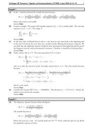
The filter w = ˆw 0 w 1 w 2 ...˜T which minimizes the estimation 

error e(n), suchthattheoutputsignaly(n) resembles the desired 

signal d(n) as much as possible is searched for. 

In order to determine the optimal filter a cost function J, whichpunish 

the deviation e(n), isintroduced.Thelargere(n), thehighercost. 

From OSB you know some different strategies, e.g., 

• The total squared error (LS) Deterministic description of the 

signal. 

X 

n 2 

J = e 2 (n) 

n 1 

• Mean squared error (MS) Stochastic description of the signal. 

J = E{|e(n)| 2 } 

• Mean squared error with extra contraint 

J = E{|e(n)| 2 }+λ|u(n)| 2 




The cost function J(n)=E{|e(n)| p } can be used for any p ≥ 1, but 

most oftenly for p =2.Thischoicegivesaconvexcostfunctionwhich 

is refered to as the Mean Squared Error. 

J = E{e(n)e ∗ (n)} = E{|e(n)| 2 } 

MSE 


In order to find the optimal filter coefficients J is minimized with 

regard to themselves. This is done by differentiating J with regard to 

w 0 , w 1 ,...,andthenbysettingthederivativetozero.Here,itis 

important that the cost function is convex, i.e., so that there is a global 

minimum. 

The minimization is expressed in terms of the gradient operator ∇, 

∇J =0 

where ∇J is called gradient vector. 

In particular, the choice of the squared cost function Mean Squared 

Error leads to the Wiener-Hopf equation-system. 




In matrix form, the cost function J = E{|e(n)| 2 } can be written 

J(w)=E{[d(n)−w H u(n)][d(n)−w H u(n)] ∗ } 

= σd 2 −wH p−p H w+w H Rw 

där 

w = ˆw 0 w 1 ... w M−1˜T M × 1 

u(n)=ˆu(n) u(n − 1) ... u(n − M +1)˜T M × 1 

2 

3 

r(0) r(1) ... r(M − 1) 

R = E{u(n)u H r ∗ (1) r(0) r(M − 2) 

(n)} = 6 

4 

. 

. 

. . 

7 

. . 

r ∗ (M − 1) r ∗ 5 

(M − 2) ... r(0) 

p = E{u(n)d ∗ (n)} = ˆp(0) p(−1) ... p(−(M − 1))˜T M × 1 


The gradient operator yields 

∇J(w)=2 ∂J(w) 

∂w ∗ =2 ∂ 

∂w ∗ (σ2 d −wH p−p H w+w H Rw) 

= −2p +2Rw 

If the gradient vector is set to zero, the Wiener-Hopf equation system 

results 

Rw o = p Wiener-Hopf 

which solution is the Wiener filter. 

w o = R −1 p 

Wienerfilter 

In other words, the Wiener filter is optimal when the cost is controlled 

by MSE. 

σ 2 d = E{d(n)d∗ (n)} 




The cost function’s dependence on the filter coefficients w can be made 

clear if written in canonical form 


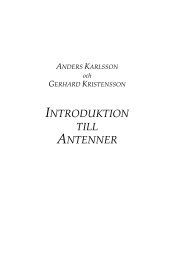
Error-Performance Surface för FIR-filter with two coefficients, 

J(w) =σ 2 d −wH p−p H w+w H Rw 

4 

14 

15 

3.5 

12 

= σ 2 d −pH R −1 p+(w−w o) H R(w−w o) 

Here, Wiener-Hopf and the expression of the Wienerfilter have been 

used in addition to the fact that the following decomposition canbe 

made 

w H Rw =(w−w o) H R(w−w o)−w H o Rwo+wH o Rw+wH Rw o 

J(w) 

10 

5 

0 

4 

w =[w 0 , w 1 ] T 0 

w0 

−4 

−3 

0.5 

3 

−2 

2 

0 

1 

−1 

0 −1 −2 

w 0 

0 w 1 w 1 

3 

2.5 

2 

1.5 

1 

w o 

−3 

−4 

10 

8 

6 

4 

2 

With the optimal filter w = w o the minimal error J min is achieved: 

J min ≡ J(w o)=σd 2 − pH R −1 p MMSE 


p = ˆ0.5272 

−0.4458˜T 

R = 

» 1.1 

– 0.5 

0.5 1.1 

w o = ˆ0.8360 −0.7853˜T Jmin =0.1579 

σ 2 d =0.9486 


Steepest Descent 17 

Steepest Descent 18 

The method of the Steepest descent is a recursive method to find 

the Wienerfiltret when the statistics of the signals are known. 

The method of the Steepest descent is not an adaptive filter, but serves 

as a basis for the LMS algorithm which is presented in Lecture 2. 

The method of the Steepest descent is a recursive method that leads 

to the Wiener-Hopfs equations. The statistics are known (R, p). The 

purpose is to avoid inversion of R. (savescomputations) 

• Set start values for the filter coefficients, w(0) (n =0) 

• Determine the gradient ∇J(n) that points in the direction in 

which the cost function increases the most. ∇J(n)=−2p+ 

2Rw(n) 

• Adjust w(n +1) in the opposite direction to the gradient, but 

weight down the adjustment with the stepsize parameter µ 

w(n+1)=w(n)+ 1 2 µ[−∇J(n)] 

• Repete steps 2 and 3. 



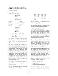
Convergence, filter coefficients 19 

Since the method of the Steepest Descent contains feedback, there 

is a risk that the algorithm diverges. This limits the choices ofthe 

stepsize parameter µ. One example of the critical choice of µ is 

given below. The statistics are the same as in the previous example. 

w(n) 

wo 0 

0 

µ =1.5 

µ =0.1 

µ =1.0 

µ =1.25 

wo 1 

0 20 40 60 80 100 

Iteration n 

» – 0.5272 

p = 

−0.4458 

» – 1.1 0.5 

R = 

0.5 1.1 

» – 0.8360 

w o = 

−0.7853 

» 0 

w(0) = 

0– 

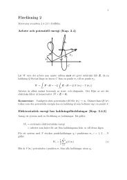
Convergence, error surface 20 

The influence of the stepsize parameter on the convergence can beseen 

when analyzing J(w). The example below illustrates the convergence 

towards J min for different choices of µ. 

w 0 

2 

1.5 

1 

0.5 

0 

-0.5 

-1 

-1.5 

wo 

µ =0.1 

µ =0.5 

µ =1.0 

w(0) 

-2 

-2 -1.5 -1 -0.5 0 0.5 1 1.5 

w 1 

2 

» – 0.5272 

p = 

−0.4458 

» – 1.1 0.5 

R = 

0.5 1.1 

» – 0.8360 

w o = 

−0.7853 

» – 1 

w(0)= 

1.7 



Convergence analysis 21 

Convergence analysis 22 

How should µ be chosen? A small value gives slow convergence, while 

alargevalueconstitutesariskfordivergence. 

Perform an eigenvalue decomposition of R in the expression of 

J(w(n)) 

J(n)=J min +(w(n)−w o) H R(w(n)−w o) 

= J min +(w(n)−w o) H QΛQ H (w(n)−w o) 

= J min + ν H (n)Λν(n)=J min + X k 

λ k |ν k (n)| 2 

The convergence of the cost function depends on ν(n), i.e., the 

convergence of w(n) through the relationship ν(n)=Q H (w(n)− 

w o). 


With the observation that w(n)=Qν(n)+w o the update of the cost 

function can be derived: 

w(n+1)=w(n)+µ[p−Rw(n)] 

Qν(n+1)+w o = Qν(n)+w o+µ[p−RQν(n) − Rw o] 

ν(n+1)=ν(n) − µQ H RQν(n) =(I − µΛ)ν(n) 

ν k (n +1)=(1− µλ k )ν k (n) (Elementk i ν(n) ) 

The latter is a 1:st order difference equation, with the solution 

ν k (n)=(1 − µλ k ) n ν k (0) 

For this equation to converge it is required that |1 − µλ k | < 1, which 

leads to the stability criterion of the method of the Steepest Descent: 

0

Summary Lecture 1 25 

Repetition av OSB 

• Quadratic cost function, J = E{|e(n)| 2 } 

• Definition of u(n), w, R and p 

• The correlations R and p is assumed to be known in advance. 

• The Gradient vector ∇J 

• Optimal filter coefficients is given by w o = R −1 p 

• Optimal (minimal) cost J min ≠0 


Summary Lecture 1 26 

Summary of the method of the Steepest Descent 

• Recursive solution to the Wiener filter 

• The statistics (R och p) isassumedtobeknown 

• The gradient vector ∇J(n) is timedependent but deterministic, 

oand points in the direction in which the cost function increases 

the most. 

• Recursion of filter veights: w(n+1)=w(n)+ 1 2 µ[−∇J(n)] 

• The cost function J(n) → J min , n → ∞, dvs w(n) → 

w o, n →∞ 

• For convergence it is required that the stepsize satisfies 0

Exempel: Inversmodellering 29 

Exempel: Modellering/Identifiering 30 

Fördröjning 

Exciterande signal 

✲ 

z −∆ 

d(n) 

u(n) 

✲ 

Undersökt 

system 

d(n) 

Undersökt u(n) 

+ 

FIR 

✎☞ 

✲ ✲ d(n) b 

system 

filter 

– 

✲ ❄ 

✍✌ Σ 

✁ ✁✁✁✁✁✁✕ 

✲ 

FIR 

filter 

✁ ✁✁✁✁✁✁✕ 

bd(n) 

+ ✎☞ ❄ 

✲ 

– ✍✌ Σ 

✲ 

Adaptiv 

algoritm 

✛ 

e(n) 

✲ 

Adaptiv 

algoritm 

✛ 

e(n) 

Vid inversmodellering kopplas det adaptiva filtret i kaskad med det 

undersökta systemet. Har systemet endast poler, kan ett adaptivt filter 

av motsvarande ordning användas. 

Adaptive Signal Processing 2013 Bilaga, Föreläsning 1 

Vid modellering/identifiering kopplas det adaptiva filtret parallellt med 

det undersökta systemet. Om det undersökta systemet endast har 

nollställen, så är det lämpligt att använda motsvarande längd på filtret. 

Har systemet både poler och nollställen krävs i regel ett långt adaptivt 

FIR-filter. 


Exempel: Ekosläckare I 31 

Exempel: Ekosläckare II 32 

u(n) Talare 1 

u(n) Talare 1 

✲ 

 

❅ ❅ 

✛ 

✲ 

✲ 

FIR 

filter 

✁ ✁✁✁✁✁✁✕ 

Adaptiv 

algoritm 

✛ 

e(n) 

bd(n) 

Hybrid 

– 

✎☞ ❄ 

✍✌ Σ 

d(n) 

✛ 

+ 

❄ 

✲ 

✛ 

Talare 2 

Vid telefoni så läcker talet från Talare 1 igenom vid hybriden. Talare 1 

kommer då att höra sin egen röst som ett eko. Detta vill man ta bort. 

Normalt stoppas adaptionen då Talare 2 pratar. Filtreringen sker dock 

under hela tiden. 


✛ 

✲ 

✲ 

FIR 

filter 

✁ ✁✁✁✁✁✁✕ 

Adaptiv 

algoritm 

✛ 

e(n) 

bd(n) 

❄ 

Impulssvar 

Ekoväg 

+ 

✎☞ ❄ Talare 2 

– ✍✌ Σ ✛ 

+ 

✎☞ ❄ 

✍✌ Σ 

d(n) ✎☞ 

✛ 

✛ + ✍✌ 

Denna struktur är tillämpbar på högtalartelefoner, videokonferenssystem 

och dylikt. Precis som vid telefonifallet hör Talare 1 sig själv i form av 

ett eko. Dock är denna effekt mer påtaglig här, eftersom mikrofonen 

fångar upp det som sänds ut av högtalaren. Adaptionen stoppas normalt 

när Talare 2 pratar, men filtreringen sker under hela tiden. 

Adaptive Signal Processing 2013 Bilaga, Föreläsning 1

Exempel: Adaptive Line Enhancer 33 

Exempel: Kanalutjämnare (Equalizer) 34 

v(n) Färgad störning 

Periodisk 

signal + ✎☞ 

✲ ❄ ✛ 

✲ 

s(n) 

+ ✍✌ Σ 

✚ 

d(n) 

❄ 

+ ❄ 

FIR 

z −∆ u(n) 

bd(n) ✎☞ 

✲ 

✲ 

filter 

– ✍✌ Σ 

Fördröjning 

✁ ✁✁✁✁✁✁✕ 

✲ 

Adaptiv 

algoritm 

✛ 

e(n) 

p(n) 

Sluten under “träning” 

✲ 

Kanal 

C(z) 

Brus v(n) 

✟ ✟✟✯ 

✲ 

z −∆ 

+ ✎☞ u(n) 

FIR 

bd(n) 

+ ✎☞ ❄ 

✲ 

✍✌ Σ ✲ 

✲ 

filter – ✍✌ Σ 

✻+ 

✁ ✁✁✁✁✁✁✕ 

✲ 

Fördröjning 

Adaptiv 

algoritm 

d(n) 

e(n) 

✛ 

Information i form av en periodisk signal störs av ett färgat brus som 

är korrelerat med sig själv inom en viss tidsram. Genom att fördröja 

signalen så pass mycket att bruset (i u(n) respektive d(n)) blir 

okorrelerat, kan bruset tryckas ned genom linjär prediktion. 

En känd pseudo noise-sekvens används för att skatta en invers modell av 

kanalen (“träning”). Därefter stoppas adaptionen, men filtret fortsätter 

att verka på den översända signalen. Syftet är att ta bort kanalens 

inverkan på den översända signalen. 


Adaptive Signal Processing 2013 Bilaga, Föreläsning 1

Welcome to Adaptive Signal Processing! Lectures and exercises ...

Create successful ePaper yourself

Delete template?

Save as template?