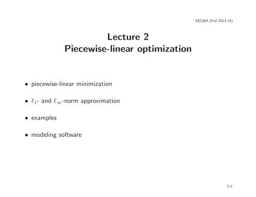
Lecture 2 Piecewise-linear optimization

EE236A (Fall 2013-14)
Lecture 2
Piecewise-linear optimization
• piecewise-linear minimization
• l 1 - and l ∞ -norm approximation
• examples
• modeling software
2–1

Linear and affine functions
linear function: a function f : R n → R is linear if
f(αx+βy) = αf(x)+βf(y)
∀x,y ∈ R n ,α,β ∈ R
property: f is linear if and only if f(x) = a T x for some a
affine function: a function f : R n → R is affine if
f(αx+(1−α)y) = αf(x)+(1−α)f(y)
∀x,y ∈ R n ,α ∈ R
property: f is affine if and only if f(x) = a T x+b for some a, b
Piecewise-linear optimization 2–2

Piecewise-linear function
f : R n → R is (convex) piecewise-linear if it can be expressed as
f(x) = max
i=1,...,m (aT i x+b i )
f is parameterized by m n-vectors a i and m scalars b i
f(x)
a T i x + b i
x
(the term piecewise-affine is more accurate but less common)
Piecewise-linear optimization 2–3

Piecewise-linear minimization
minimize f(x) = max
i=1,...,m (aT i x+b i )
• equivalent LP (with variables x and auxiliary scalar variable t)
minimize t
subject to a T i x+b i ≤ t, i = 1,...,m
to see equivalence, note that for fixed x the optimal t is t = f(x)
• LP in matrix notation: minimize ˜c T˜x subject to Øx ≤˜b with
˜x =
[
x
t
] [
0
, ˜c =
1
⎡
]
, Ã =
−1
. .
a T m −1
⎣ aT 1
⎤ ⎡
⎦, ˜b = ⎣ −b ⎤
1
. ⎦
−b m
Piecewise-linear optimization 2–4

Minimizing a sum of piecewise-linear functions
minimize f(x)+g(x) = max
i=1,...,m (aT i x+b i )+ max
i=1,...,p (cT i x+d i )
• cost function is piecewise-linear: maximum of mp affine functions
(
f(x)+g(x) = max (ai +c j ) T x+(b i +d j ) )
i=1,...,m
j=1,...,p
• equivalent LP with m+p inequalities
minimize t 1 +t 2
subject to a T i x+b i ≤ t 1 , i = 1,...,m
c T i x+d i ≤ t 2 , i = 1,...,p
note that for fixed x, optimal t 1 , t 2 are t 1 = f(x), t 2 = g(x)
Piecewise-linear optimization 2–5

• equivalent LP in matrix notation
minimize ˜c T˜x
subject to Øx ≤˜b
with
˜x =
⎡
⎣ x ⎤
t 1
⎦, ˜c =
t 2
⎡
⎣ 0 1
1
⎤
⎦, Ã =
⎡
⎢
⎣
a T 1 −1 0
. . .
a T m −1 0
c T 1 0 −1
. . .
0 −1
c T p
⎤ ⎡
, ˜b = ⎥ ⎢
⎦ ⎣
⎤
−b 1
.
−b m
−d 1
⎥
. ⎦
−d p
Piecewise-linear optimization 2–6

l ∞ -Norm (Cheybshev) approximation
with A ∈ R m×n , b ∈ R m
minimize ‖Ax−b‖ ∞
• l ∞ -norm (Chebyshev norm) of m-vector y is
‖y‖ ∞ = max
i=1,...,m |y i| = max
i=1,...,m max{y i,−y i }
• equivalent LP (with variables x and auxiliary scalar variable t)
minimize t
subject to −t1 ≤ Ax−b ≤ t1
(for fixed x, optimal t is t = ‖Ax−b‖ ∞ )
Piecewise-linear optimization 2–7

• equivalent LP in matrix notation
minimize
[
0
1
] T [
x
t
]
subject to
[
A −1
−A −1
][
x
t
]
≤
[
b
−b
]
Piecewise-linear optimization 2–8

l 1 -Norm approximation
minimize ‖Ax−b‖ 1
• l 1 -norm of m-vector y is
‖y‖ 1 =
m∑
|y i | =
i=1
m∑
max{y i ,−y i }
i=1
• equivalent LP (with variable x and auxiliary vector variable u)
minimize
m∑
u i
i=1
subject to −u ≤ Ax−b ≤ u
(for fixed x, optimal u is u i = |(Ax−b) i |, i = 1,...,m)
Piecewise-linear optimization 2–9

• equivalent LP in matrix notation
minimize
[
0
1
] T [
x
u
]
subject to
[
A −I
−A −I
][
x
u
]
≤
[
b
−b
]
Piecewise-linear optimization 2–10

Comparison with least-squares solution
histograms of residuals Ax−b, with randomly generated A ∈ R 200×80 , for
10
8
6
4
2
01.5
100
80
60
40
20
¡1.5 0
x ls = argmin‖Ax−b‖, x l1 = argmin‖Ax−b‖ 1
1.0
0.5 0.0 0.5 1.0 1.5
(Ax ls −b) k
¡¡1.0
0.5 0.0 0.5 1.0 1.5
(Ax l1 −b) k
l 1 -norm distribution is wider with a high peak at zero
Piecewise-linear optimization 2–11

Robust curve fitting
• fit affine function f(t) = α+βt to m points (t i ,y i )
• an approximation problem Ax ≈ b with
⎡
A = ⎣ 1 t ⎤
[
1 α
. . ⎦, x =
β
1 t m
]
, b =
⎡
⎣ y ⎤
1
. ⎦
y m
f(t)
25
20
15
10
5
0
¢5
¢10
¢15
¢20
¢10
¢5 0 5 10
t
• dashed: minimize ‖Ax−b‖
• solid: minimize ‖Ax−b‖ 1
l 1 -norm approximation is more
robust against outliers
Piecewise-linear optimization 2–12

Sparse signal recovery via l 1 -norm minimization
• ˆx ∈ R n is unknown signal, known to be very sparse
• we make linear measurements y = Aˆx with A ∈ R m×n , m < n
estimation by l 1 -norm minimization: compute estimate by solving
minimize ‖x‖ 1
subject to Ax = y
estimate is signal with smallest l 1 -norm, consistent with measurements
equivalent LP (variables x, u ∈ R n )
minimize 1 T u
subject to −u ≤ x ≤ u
Ax = y
Piecewise-linear optimization 2–13

Example
2
• exact signal ˆx ∈ R 1000
• 10 nonzero components
ˆxk
1
0
−1
−2
0 200 400 600 800 1000
k
least-norm solutions (randomly generated A ∈ R 100×1000 )
minimum l 2 -norm solution
minimum l 1 -norm solution
2
2
1
1
xk
0
xk
0
−1
−1
−2
0 200 400 600 800 1000
k
−2
0 200 400 600 800 1000
k
l 1 -norm estimate is exact
Piecewise-linear optimization 2–14

Exact recovery
when are the following problems equivalent?
minimize card(x)
subject to Ax = y
minimize ‖x‖ 1
subject to Ax = y
• card(x) is cardinality (number of nonzero components) of x
• depends on A and cardinality of sparsest solution of Ax = y
we say A allows exact recovery of k-sparse vectors if
ˆx = argmin
Ax=y
‖x‖ 1
when y = Aˆx and card(ˆx) ≤ k
• here, argmin‖x‖ 1 denotes the unique minimizer
• a property of (the nullspace) of the ‘measurement matrix’ A
Piecewise-linear optimization 2–15

‘Nullspace condition’ for exact recovery
necessary and sufficient condition for exact recovery of k-sparse vectors 1
|z (1) |+···+|z (k) | < 1 2 ‖z‖ 1 ∀z ∈ nullspace(A)\{0}
here, z (i) denotes component z i in order of decreasing magnitude
|z (1) | ≥ |z (2) | ≥ ··· ≥ |z (n) |
• a bound on how ‘concentrated’ nonzero vectors in nullspace(A) can be
• implies k < n/2
• difficult to verify for general A
• holds with high probability for certain distributions of random A
1 Feuer & Nemirovski (IEEE Trans. IT, 2003) and several other papers on compressed sensing.
Piecewise-linear optimization 2–16

Proof of nullspace condition
notation
• x has support I ⊆ {1,2,...,n} if x i = 0 for i ∉ I
• |I| is number of elements in I
• P I is projection matrix on n-vectors with support I: P I is diagonal with
(P I ) jj =
{
1 j ∈ I
0 otherwise
• A satisfies the nullspace condition if
‖P I z‖ 1 < 1 2 ‖z‖ 1
for all nonzero z in nullspace(A) and for all support sets I with |I| ≤ k
Piecewise-linear optimization 2–17

sufficiency: suppose A satisfies the nullspace condition
• let ˆx be k-sparse with support I (i.e., with P Iˆx = ˆx); define y = Aˆx
• consider any feasible x (i.e., satisfying Ax = y), different from ˆx
• define z = x− ˆx; this is a nonzero vector in nullspace(A)
‖x‖ 1 = ‖ˆx+z‖ 1
≥ ‖ˆx+z −P I z‖ 1 −‖P I z‖ 1
= ∑ k∈I
|ˆx k |+ ∑ k∉I
|z k |−‖P I z‖ 1
= ‖ˆx‖ 1 +‖z‖ 1 −2‖P I z‖ 1
> ‖ˆx‖ 1
(line 2 is the triangle inequality; the last line is the nullspace condition)
therefore ˆx = argmin Ax=y ‖x‖ 1
Piecewise-linear optimization 2–18

necessity: suppose A does not satisfy the nullspace condition
• for some nonzero z ∈ nullspace(A) and support set I with |I| ≤ k,
‖P I z‖ 1 ≥ 1 2 ‖z‖ 1
• define a k-sparse vector ˆx = −P I z and y = Aˆx
• the vector x = ˆx+z satisfies Ax = y and has l 1 -norm
‖x‖ 1 = ‖−P I z +z‖ 1
= ‖z‖ 1 −‖P I z‖ 1
≤ 2‖P I z‖ 1 −‖P I z‖ 1
= ‖ˆx‖ 1
therefore ˆx is not the unique l 1 -minimizer
Piecewise-linear optimization 2–19

Linear classification
• given a set of points {v 1 ,...,v N } with binary labels s i ∈ {−1,1}
• find hyperplane that strictly separates the two classes
a T v i +b > 0 if s i = 1
a T v i +b < 0 if s i = −1
homogeneous in a, b, hence equivalent to the linear inequalities (in a, b)
s i (a T v i +b) ≥ 1, i = 1,...,N
Piecewise-linear optimization 2–20

Approximate linear separation of non-separable sets
minimize
N∑
max{0,1−s i (a T v i +b)}
i=1
• penalty 1−s i (a T i v i+b) for misclassifying point v i
• can be interpreted as a heuristic for minimizing #misclassified points
• a piecewise-linear minimization problem with variables a, b
Piecewise-linear optimization 2–21

equivalent LP (variables a ∈ R n , b ∈ R, u ∈ R N )
minimize
N∑
u i
i=1
subject to 1−s i (v T i a+b) ≤ u i, i = 1,...,N
u i ≥ 0, i = 1,...,N
in matrix notation:
⎡
⎤
T ⎡
⎤
minimize
subject to
⎣ 0 0 ⎦ ⎣ a b ⎦
1 u
⎡
−s 1 v1 T −s 1 −1 0 ··· 0
−s 2 v2 T −s 2 0 −1 ··· 0
. . . . ... .
−s N vN T −s N 0 0 ··· −1
0 0 −1 0 ··· 0
⎢ 0 0 0 −1 ··· 0
⎣ . . . . ... .
0 0 0 0 ··· −1
⎤
⎡
⎢
⎣
⎥
⎦
⎤
a
b
u 1
u 2
⎥
. ⎦
u N
≤
⎡
⎢
⎣
−1
−1
.
−1
0
0.
0
⎤
⎥
⎦
Piecewise-linear optimization 2–22

Modeling software
modeling tools simplify the formulation of LPs (and other problems)
• accept optimization problem in standard notation (max, ‖·‖ 1 , . . . )
• recognize problems that can be converted to LPs
• express the problem in the input format required by a specific LP solver
examples of modeling packages
• AMPL, GAMS
• CVX, YALMIP (MATLAB)
• CVXPY, Pyomo, CVXOPT (Python)
Piecewise-linear optimization 2–23

CVX example
minimize ‖Ax−b‖ 1
subject to 0 ≤ x k ≤ 1, k = 1,...,n
MATLAB code
cvx_begin
variable x(n);
minimize( norm(A*x - b, 1) )
subject to
x >= 0
x