CEPAL Review 109.indb
CEPAL Review 109.indb
CEPAL Review 109.indb

You also want an ePaper? Increase the reach of your titles
YUMPU automatically turns print PDFs into web optimized ePapers that Google loves.
REVIEW<br />
ECONOMIC<br />
COMMISSION FOR<br />
LATIN AMERICA<br />
AND THE CARIBBEAN
109<br />
N O<br />
APRIL • 2013<br />
REVIEW<br />
Alicia Bárcena<br />
Executive Secretary<br />
Antonio Prado<br />
Deputy Executive Secretary<br />
ECONOMIC<br />
COMMISSION FOR<br />
LATIN AMERICA<br />
AND THE CARIBBEAN<br />
Osvaldo Sunkel<br />
Chairman of the Editorial Board<br />
André Hofman<br />
Director<br />
Miguel Torres<br />
Technical Editor<br />
ISSN 0251-2920
The cepal <strong>Review</strong> was founded in 1976, along with the corresponding Spanish version, Revista de la cepal, and is published three<br />
times a year by the United Nations Economic Commission for Latin America and the Caribbean, which has its headquarters in<br />
Santiago, Chile. The <strong>Review</strong>, however, has full editorial independence and follows the usual academic procedures and criteria,<br />
including the review of articles by independent external referees. The purpose of the <strong>Review</strong> is to contribute to the discussion of<br />
socio-economic development issues in the region by offering analytical and policy approaches and articles by economists and other<br />
social scientists working both within and outside the United Nations. The <strong>Review</strong> is distributed to universities, research institutes<br />
and other international organizations, as well as to individual subscribers.<br />
The opinions expressed in the signed articles are those of the authors and do not necessarily reflect the views of the organization. The<br />
designations employed and the way in which data are presented do not imply the expression of any opinion whatsoever on the part<br />
of the secretariat concerning the legal status of any country, territory, city or area or its authorities, or concerning the delimitation<br />
of its frontiers or boundaries.<br />
A subscription to the cepal <strong>Review</strong> in Spanish costs US$ 30 for one year (three issues) and US$ 50 for two years. A subscription<br />
to the English version costs US$ 35 or US$ 60, respectively. The price of a single issue in either Spanish or English is US$ 15,<br />
including postage and handling.<br />
The complete text of the <strong>Review</strong> can also be downloaded free of charge from the eclac web site (www.cepal.org).<br />
This publication, entitled the cepal <strong>Review</strong>, is covered in the<br />
Social Sciences Citation Index (ssci), published by Thomson<br />
Reuters, and in the Journal of Economic Literature (jel),<br />
published by the American Economic Association<br />
To subscribe, please apply to eclac Publications, Casilla 179-D,<br />
Santiago, Chile, by fax to (562) 210-2069 or by e-mail to<br />
publications@eclac.cl. The subscription form may be requested by<br />
mail or e-mail or can be downloaded from the <strong>Review</strong>’s Web page:<br />
http://www.cepal.org/revista/noticias/paginas/5/20365/suscripcion.pdf.<br />
United Nations publication<br />
ISSN 0251-2920<br />
ISBN 978-92-1-221069-8<br />
e-ISBN 978-92-1-056008-5<br />
LC/G.2556-P<br />
Copyright © United Nations, April 2013. All rights reserved.<br />
Printed in Santiago, Chile<br />
Requests for authorization to reproduce this work in whole or in part should be sent to the Secretary of the Publications Board.<br />
Member States and their governmental institutions may reproduce this work without prior authorization, but are requested to mention<br />
the source and to inform the United Nations of such reproduction. In all cases, the United Nations remains the owner of the copyright<br />
and should be identified as such in reproductions with the expression “© United Nations 2013”.
<strong>CEPAL</strong> review 109<br />
5<br />
Articles<br />
Capital formation in Latin America: one and a half century<br />
of macroeconomic dynamics<br />
Xavier Tafunell 7<br />
Economic growth and the environment<br />
Adolfo Figueroa 27<br />
Internationalization and technology in mercosur<br />
Isabel Álvarez , Bruno B. Fischer and José Miguel Natera 41<br />
Productive structure and the functional distribution of income:<br />
an application of the input-output model<br />
Pedro Quaresma de Araujo 57<br />
Income polarization, the middle class and informal employment<br />
in Greater Buenos Aires, 1974-2010<br />
Fernando Groisman 79<br />
Inequality and academic achievement in Chile<br />
Pablo Muñoz H. and Amaia Redondo S. 99<br />
Determinants of structural heterogeneity in Mexican<br />
manufacturing industry, 1994-2008<br />
Raúl Vázquez López 115<br />
Mexico: Value added in exports of manufactures<br />
Gerardo Fujii G. and Rosario Cervantes M. 131<br />
The political economy of regional grants in Peru<br />
Leonardo E. Letelier S. and Gonzalo Neyra A. 147<br />
Chile: is the fee for non-use of water rights effective?<br />
Christian Valenzuela, Rodrigo Fuster and Alejandro León 163<br />
Guidelines for contributors to the cepal <strong>Review</strong> 187<br />
april 2013
Explanatory notes<br />
The following symbols are used in tables in the <strong>Review</strong>:<br />
… Three dots indicate that data are not available or are not separately reported.<br />
(–) A dash indicates that the amount is nil or negligible.<br />
A blank space in a table means that the item in question is not applicable.<br />
(-) A minus sign indicates a deficit or decrease, unless otherwise specified.<br />
(.) A point is used to indicate decimals.<br />
(/) A slash indicates a crop year or fiscal year; e.g., 2006/2007.<br />
(-) Use of a hyphen between years (e.g., 2006-2007) indicates reference to the complete period considered, including the beginning<br />
and end years.<br />
The word “tons” means metric tons and the word “dollars” means United States dollars, unless otherwise stated. References to annual<br />
rates of growth or variation signify compound annual rates. Individual figures and percentages in tables do not necessarily add up to<br />
the corresponding totals because of rounding.
cepal review 109 • april 2013 7<br />
Capital formation in Latin America: one and a<br />
half century of macroeconomic dynamics<br />
Xavier Tafunell<br />
Abstract<br />
Macroeconomic studies indicate that physical capital formation has played a pivotal<br />
role in long-term economic growth. These studies have been hampered, however,<br />
by a data constraint: in order to pinpoint exactly what the role of capital formation<br />
has been, a larger empirical database –larger in terms of both the time span and<br />
the geographical area covered– is needed. This study addresses that problem by<br />
providing new and very extensive series on capital formation in Latin America. It<br />
also describes the different series used to identify long, medium and short-term<br />
movements. One of the outstanding features of these investment trends were their<br />
marked instability up to 1950. Another salient aspect has been the more robust<br />
growth in investment seen in the second half of the nineteenth century, which actually<br />
outdistanced the growth spurt that occurred during the “golden age” of 1950-1980.<br />
KEYWORDs<br />
Economic growth, macroeconomics, capital, capital formation, capital movements, investments, measurement,<br />
statistics, Latin America<br />
JEL CLAssIFICATION<br />
E2, N16, N66<br />
AUTHOR<br />
Xavier Tafunell is a Professor of Economic History in the Department of Economics and Business of the<br />
Universitat Pompeu Fabra in Barcelona, Spain. xavier.tafunell@upf.edu
8<br />
cepal review 109 • april 2013<br />
I<br />
Introduction<br />
Economic historians and specialists in the macroeconomics<br />
of development are continually trying to identify the<br />
explanatory forces behind long-term growth. Ever<br />
since the time of the classical economists, the idea that<br />
physical capital formation is one of the determinants<br />
of growth has been in the air. Economists who have<br />
sought to analyse this question empirically have used<br />
one of two approaches: growth regressions or growth<br />
accounting. The vast number of studies that have taken<br />
the first of these approaches have looked at a wide range<br />
of variables, but one of the few variables that is almost<br />
never omitted is investment, either as a flow or a stock<br />
(Levine and Renelt, 1992). In a study that employed<br />
various permutations to combine the variables used in<br />
all the different models (Sala-i-Martín, 1997), the author<br />
concludes that investment in equipment is the variable<br />
that is the most closely correlated with gross domestic<br />
product (gdp). More recently, Qi (2007) –as had Temple<br />
and Voth (1998) before her– has found that the link between<br />
growth and long-term capital formation is stronger in<br />
developing economies. In fact, no macroeconomist who<br />
has studied this subject has questioned the existence of<br />
a close, statistically robust relationship between capital<br />
formation and gdp. The issue on which they are not in<br />
agreement is the underlying causality; in other words,<br />
the role that physical capital formation plays in driving<br />
growth (Bosworth and Collins, 2003). This debate<br />
cannot, in all likelihood, be resolved until a broader<br />
spatio-temporal database can be constructed – one that<br />
incorporates very long-term series on investment in<br />
developing countries such as the Latin American nations.<br />
A review of the studies done using a growth<br />
accounting approach leads to the same conclusion even<br />
more clearly. Studies on industrialized economies show<br />
that total factor productivity has been the main driver<br />
Funding for this study has been provided by the Ministry of Science<br />
and Innovation of Spain (Project No. ECO2010-15882). Assistance<br />
was provided by Marc Badia, Cristián Ducoing and César Yáñez in<br />
locating and reproducing statistics. Sandra Kuntz was kind enough to<br />
provide a digital copy of statistics for Mexico which were otherwise<br />
unavailable. José Jofré, Frank Notten and Carolina Román helped to<br />
build the databases. The author is partially responsible for the data<br />
compiled and bears sole responsibility for the way in which they have<br />
been processed and for any errors that may be found in these series.<br />
The suggestions made by an anonymous cepal <strong>Review</strong> referee were<br />
also extremely useful.<br />
of growth throughout the twentieth century (Kendrik,<br />
1993). Nonetheless, in all regions of the world other than<br />
the geographical area covered by the Organisation for<br />
Economic Cooperation and Development (oecd), physical<br />
capital formation has played a central role in driving<br />
growth, even during the second half of the twentieth<br />
century (Bosworth and Collins, 2003). The experiences<br />
of countries in Africa (Abu-Qarn and Abu-Bader, 2007)<br />
and Asia, both in relation to the “tigers” of South-East<br />
Asia and the two Asian giants (China and India), 1 are<br />
informative. There are thus sound reasons for positing<br />
that physical capital formation has been one of the main<br />
sources of economic growth in Latin America during the<br />
past 150 years. The few growth-accounting studies on<br />
the subject for the second half of the twentieth century<br />
point in this direction. According to Elías (1992), physical<br />
capital formation was the most important determinant<br />
of growth in the region’s major economies between<br />
1940 and 1985. Hofman (2000), who used a much more<br />
sophisticated methodology, also found that capital was<br />
the most influential factor of production, although he<br />
calculated its contribution as being much smaller. In a<br />
study that, unlike any of its predecessors, took in all of<br />
the Latin American countries except Cuba for the period<br />
from 1960 to 2000, Loayza, Fajnzylber and Calderón<br />
(2005) found that capital and labour were more or less<br />
on a par in terms of their contribution to growth, whereas<br />
multifactor productivity did very little to spur growth.<br />
The aim of this study is to provide the academic<br />
community with an extensive body of fresh empirical<br />
evidence on Latin American countries’ investment flows<br />
so that scholars looking at long-term growth trends in<br />
these economies will have very long-term data series<br />
on this fundamental explanatory factor. As is well<br />
known, thanks to the series compiled and reworked by<br />
Maddison (2007), we still lack estimated gdp series for<br />
the vast majority of Latin American countries for the<br />
second half of the nineteenth century and even for the<br />
early twentieth century in some cases. As a result, the<br />
series on capital formation presented here do not shed<br />
1 Regarding the South-East Asian economies, see Krugman (1994),<br />
Kim and Landau (1994), Young (1994 and 1995), Collins and Bosworth<br />
(1996) and Fukuda and Toya (1998). For China and India, see Bosworth<br />
and Collins (2008).<br />
Capital formation in Latin America: one and a half century<br />
of macroeconomic dynamics • Xavier Tafunell
cepal review 109 • april 2013<br />
9<br />
light on the links between capital formation and gdp, but<br />
rather on a much simpler and more basic question: the<br />
approximate trends in gdp in Latin American economies<br />
during the years when the capability of measuring them<br />
was not yet in place.<br />
This article is structured very simply. Section II<br />
describes the method used to estimate gross fixed capital<br />
formation (gfcf) for the “pre-statistics era” (the years<br />
before official national accounts were kept). Section<br />
III covers the long-term trends in gfcf for 1856-2008.<br />
Section IV outlines medium- and short-term movements<br />
and then offers a brief concluding review. The study<br />
closes with a table showing the series that have been<br />
compiled for use by researchers in this field.<br />
II<br />
gfcf estimates for the Latin American<br />
countries, 1856-1950<br />
gfcf estimates are usually calculated in the course of<br />
the preparation of national accounts, i.e., on the basis of<br />
gdp computations. The vast majority of Latin American<br />
countries began to keep official national accounts around<br />
1950, and they did so by following the conceptual and<br />
methodological guidelines set out by the United Nations.<br />
The support provided by the United Nations’ regional<br />
agency, the Economic Commission for Latin America<br />
and the Caribbean (eclac), proved to be a crucial factor<br />
in the success of this decentralized, collective effort.<br />
Thanks to the ongoing technical assistance and advisory<br />
services made available by eclac, together with its<br />
work in compiling and standardizing the data, the region<br />
now has a complete, comparable database on the main<br />
supply-side and demand-side components of gdp and on<br />
total gdp for all the countries of the region from 1950<br />
onward. 2 A number of authors have used these statistics<br />
to analyse the way in which capital formation and capital<br />
stocks influenced the Latin American economies’ growth<br />
during the second half of the twentieth century.<br />
The picture is a very different one for the years<br />
before 1950. Apart from the individual historical series<br />
prepared for some economies of the region, the only<br />
fairly broad-coverage homogeneous reconstruction<br />
of gfcf series is the one developed by André Hofman<br />
2 Historical series on aggregates prepared using a standardized<br />
methodology (United Nations System of National Accounts 1993<br />
(SNA,1993)) are contained in the database that can be accessed online<br />
through eclac Cuadernos estadísticos No. 37 (http://www.eclac.cl/<br />
deype/cuaderno37/esp/index.htm). The data for Cuba are limited,<br />
and the full annual series therefore usually cover 19 Latin American<br />
countries and 13 Caribbean ones. The statistics for the Caribbean<br />
nations generally date back only as far as 1970, however. There are<br />
some gaps in the series on both Latin American nations and Caribbean<br />
countries in the case of the less developed economies. For a discussion<br />
of the gaps in capital formation series, see Tafunell (2011).<br />
(2000) for 1900 and 1994 for Argentina, Brazil, Chile,<br />
Colombia, Mexico and Venezuela. The only precedent<br />
for an effort of this type was the preliminary evaluations<br />
undertaken by, once again, eclac in 1951. No study of<br />
this sort had been done on the other 14 Latin American<br />
countries, however, and, as a result, trends in capital<br />
formation for the region as a whole prior to 1950 are<br />
simply unknown.<br />
The main objective of this study is simply to<br />
determine the annual levels of fixed capital formation<br />
in all the countries of the region during a period of time<br />
preceding the introduction of official national accounts.<br />
How long should this period be? Ideally, the data should<br />
go back as far as the early nineteenth century, when these<br />
countries were in the process of becoming independent.<br />
The early statistical evidence is of such poor quality,<br />
however, that the starting point for the series has to be<br />
moved up to midway through that century: 1856, to<br />
be exact (Tafunell, 2011). The ongoing civil strife and<br />
outright chaos experienced by many of these countries<br />
up to around that time (or even later) attests to just how<br />
difficult it would be to quantify investment levels on<br />
any consistent basis during the decades following these<br />
countries’ political emancipation. 3 After calculating<br />
the gfcf up to 1950, the series were merged with the<br />
official series compiled by eclac. 4 This should by no<br />
means be interpreted as implying that the two series are<br />
of comparable quality. They have been merged simply in<br />
3 The overview provided by Dye (2006) is helpful in gaining an<br />
understanding of the difficulties involved in establish a stable institutional<br />
order. For an opposing interepretation that is highly critical of the<br />
conventional wisdom on this subject, see Deas (2010).<br />
4 This study focuses solely on the series prepared by the author (i.e.,<br />
the series for 1856-1950), since the series for years since 1950 are<br />
well-known and widely available (see footnote 2).<br />
Capital formation in Latin America: one and a half century<br />
of macroeconomic dynamics • Xavier Tafunell
10<br />
cepal review 109 • april 2013<br />
order to obtain a very long-term picture of gfcf trends.<br />
This is a legitimate exercise, in the author’s view, so long<br />
as the results of the quantification are sufficiently reliable.<br />
This statistical reconstruction provides a way of<br />
obtaining an overview of the investment activity of all<br />
the countries of Latin America, and it has proven to be<br />
an almost entirely successful approach. As shown in the<br />
tables presented here, measurements of gfcf have been<br />
obtained for 17 countries. The only ones that have been<br />
omitted are Guatemala, Panama and Paraguay. 5 Since<br />
these three small countries account for no more than a<br />
tiny fraction of the region’s total gfcf, the series presented<br />
here for 17 Latin American countries can be viewed<br />
as being representative of Latin America as a whole. 6<br />
gfcf is an economic aggregate that encompasses<br />
capital goods of various sorts which are acquired because<br />
they serve as inputs for production process, because of<br />
the length of their useful life and, above all, because they<br />
help to boost productivity in the economy as a whole<br />
thanks to their embedded technologies. In calculating<br />
the amount of capital stock that they represent, they are<br />
usually divided into four categories: machinery and related<br />
equipment, transport equipment, residential construction<br />
and non-residential construction. Hofman (2000) used<br />
this classification for his study on this subject in six of<br />
the larger Latin American economies. Unfortunately, it<br />
has not been possible –and may never be possible– to<br />
apply his methodology to the other economies of the<br />
region, especially for the years preceding the twentieth<br />
century. The quantifications that I have prepared have<br />
yielded investment series for three categories of goods:<br />
machinery and related equipment; transport equipment;<br />
and construction. Any attempt to break down this last<br />
category into residential and non-residential construction<br />
is doomed to failure because the types of indicators or<br />
information that would be needed in order to differentiate<br />
between the two are simply not available. 7 Moreover,<br />
5 Panama is not covered because the foreign trade statistics compiled<br />
by the more industrialized countries, which were the main source for<br />
the estimates up to 1929, attribute merchandise trade flows to that<br />
country that were actually directed towards other countries owing to<br />
Panama’s unique position, thanks to the Panama Canal, as a transit<br />
country. The series for Guatemala and Paraguay could not be calculated<br />
for 1930-1950 because the data were exceedingly difficult to obtain<br />
and/or process.<br />
6 My calculations (based on official statistics published by eclac)<br />
indicate that the aggregate level of investment for these three countries in<br />
1950 amounted to just 1.3% of the total for Latin America (20 countries).<br />
7 An arbitrary estimate of investment in residential construction<br />
might be derived from the growth patterns of the urban population.<br />
This would be a very tenuous approximation, however, since many<br />
countries did not carry out population censuses for many years, and<br />
very little is known about their urban population trends.<br />
the built-in limitations of the official national accounts<br />
database maintained by eclac are such that the<br />
disaggregation of gfcf can be carried only so far. The<br />
annual series available in the eclac database include<br />
just two aggregates: machinery and other equipment, and<br />
construction. As a result, the definitive series presented<br />
in this article (see the table in the annex) refer only to<br />
these two fundamental categories of capital formation.<br />
How have I gone about calculating the levels of these<br />
two types of investment? A detailed description of the<br />
sources and methods used is provided in Tafunell (2011).<br />
A much briefer outline will be provided here owing to<br />
space constraints. Official foreign trade statistics are the<br />
main –virtually only– source used for this quantification<br />
exercise, since the economies of the region presumably<br />
purchased their stock of capital goods from more<br />
industrialized economies. For the years from 1856 to<br />
1929, trade statistics for Germany, the United States and<br />
the United Kingdom have been used; for the period from<br />
1929 to 1950, the calculations are based on official trade<br />
statistics for the Latin American countries themselves.<br />
The procedure used to arrive at these estimates is based<br />
on the compilation of annual series, using indices for<br />
investment in equipment and in construction between 1856<br />
and 1950. The series have been converted into dollars at<br />
1950 prices using the level of investment for that year, in<br />
current dollars, as a unit of account (numéraire), as shown<br />
in the eclac database. The investment indices that I have<br />
ended up with are the result of the chain-linking of separate<br />
indices for 1856-1890, 1890-1929 and 1929-1950. The<br />
investment series for construction are composed of quantum<br />
indices based on imports or the apparent consumption of<br />
basic inputs (iron and steel for construction plus –from<br />
1900 on– cement). I also ran a sensitivity test for 1925-<br />
1950, comparing the volume (tons) series and the value<br />
(constant prices) series for metal inputs in order to verify<br />
that using one or the other does not affect the outcome in<br />
statistical terms. The series for investment in machinery<br />
and other equipment is based on the value of imported<br />
goods at 1913 prices for 1856-1929 and at 1950 prices<br />
for 1929-1950. 8 For Argentina, Brazil and Mexico, I took<br />
domestically produced equipment into account and, for<br />
those countries plus Chile, Colombia and Cuba, I took<br />
8 For the years from 1856 to 1929, I first computed aggregate investment<br />
figures in pounds sterling, German marks and United States dollars<br />
at current prices and then converted them into a common currency<br />
(pounds). I then deflated the resulting aggregate series using a price<br />
index for which the base year of 1913 equals 100. For 1929-1950,<br />
I also computed series at current and constant prices, with the latter<br />
being derived through the application of implicit unit values for 1950<br />
to the quantity data.<br />
Capital formation in Latin America: one and a half century<br />
of macroeconomic dynamics • Xavier Tafunell
cepal review 109 • april 2013<br />
11<br />
domestically produced iron for use in construction into<br />
account as well, since, unlike the situation in the other<br />
countries of Latin America, national producers were<br />
meeting an appreciable share of demand from the 1930s<br />
on. 9 One point that remains open for discussion, which<br />
could lead to a revision of the calculations, is whether or<br />
not investment in equipment in Chile, Cuba and Uruguay,<br />
and perhaps in some other countries such as Colombia<br />
and Peru, should also include domestic output, since it<br />
is quite likely that national producers had ceased to be of<br />
negligible importance by 1929 or even a few years before<br />
then. 10 The estimates for these countries may also have<br />
a slight downward bias because they do not incorporate<br />
the output of the railroad companies’ machine shops. 11<br />
The main methodological caveat in terms of<br />
the estimates given here has to do with a different<br />
aspect, however: investment in construction. Since<br />
my measurements are based solely on the apparent<br />
consumption of “modern” inputs, such as iron, steel and<br />
cement, they are clearly not very representative of activity<br />
in housing construction until well into the twentieth<br />
century and are actually not sufficiently representative<br />
of non-residential construction in the second half of the<br />
nineteenth century either. Given the widespread use of<br />
traditional materials during those years (stone, wood and<br />
clay), my figures on investment in construction surely,<br />
at the very least, overstate its long-term growth. 12<br />
9 For a more detailed discussion, see Tafunell (2011).<br />
10 In his recently submitted doctoral thesis, Ducoing (2012, pp.<br />
69-70) states that, before the Great Depression, Chilean producers<br />
accounted for no more than 3% of that country’s total available supply<br />
of equipment even in their best years. During the Second World War,<br />
when it became more and more difficult to import equipment, national<br />
producers’ share of the market climbed to 16%, but shrank again to<br />
less than 7% during the first decade of the post-war period.<br />
11 The studies conducted by Guajardo (1996 and 1998) provide an<br />
informative view of the role of railroad machine shops in Chile and<br />
Mexico. They indicate that, even in those countries, where it is thought<br />
that they became a force to be reckoned with, they actually accounted<br />
for no more than a small share of production.<br />
12 This points up what is quite likely an insurmoutable constraint,<br />
since statistics on the production of traditional construction materials<br />
are simply not available for this time period. It must be remembered<br />
that the large-scale use of iron and steel in infrastructure works came<br />
hand-in-hand with the laying of the railroads. For a discussion of the<br />
spread of the use of cement, see Tafunell (2007).<br />
III<br />
The long-term growth of gfcf<br />
The first aspect of the results of this quantification exercise<br />
that is of interest is the long-term growth rate of aggregate<br />
investment and the way in which it has varied. gfcf in<br />
Latin America, according to my calculations, soared by<br />
a factor of 95 between 1856 and 1950, which equates to<br />
a cumulative annual growth rate of 5.0%. Interestingly<br />
enough, this growth rate exceeds, although not by a large<br />
margin, the rate registered for the years following 1950,<br />
since between 1950 and 2008 it rose at an annual rate of<br />
4.4%. The progress made in terms of capitalization during<br />
the first stage of the globalization process (up to 1913)<br />
outpaced the advances achieved during the “golden age”<br />
of State-led industrialization and during the second stage<br />
of the globalization process in recent decades (see tables<br />
1 and 2). This clearly has to do with the “Gerschenkron<br />
effect”, since the growth potential for investment in the<br />
nineteenth century was extraordinary given the extremely<br />
low levels it had reached around 1850.<br />
Focusing on the period of 1856-1950 (since much<br />
less is known about this period than the one that followed),<br />
tables 1 and 2 show the average annual growth rates for<br />
gfcf in absolute and per-capita terms for the periods<br />
associated with the different growth phases that can<br />
be identified according to the literature. These figures<br />
show that the years 1873 and 1890 marked the turning<br />
points at which sharp, sustained surges in investment<br />
triggered serious financial crises (Marichal, 1989). The<br />
years 1913 and 1929 are so well known to have been<br />
turning points in the business cycle that it is unnecessary<br />
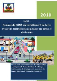
to dwell on this point here. The graph of the aggregate<br />
investment series for Latin America (see figure 1) leaves<br />
little doubt as to the appropriateness of the time-based<br />
categories shown in the tables. Clearly, figure 1 depicts<br />
major short-term movements (movements encompassing<br />
a decade or less) which we will look at again later on<br />
(see the following section).<br />
Capital formation in Latin America: one and a half century<br />
of macroeconomic dynamics • Xavier Tafunell
12<br />
cepal review 109 • april 2013<br />
TABLE 1<br />
Cumulative average annual gfcf growth rate<br />
(Percentages)<br />
Period<br />
Argentina<br />
Bolivia<br />
Brazil<br />
Chile<br />
Colombia<br />
Costa Rica<br />
Cuba<br />
Ecuador<br />
El Salvador<br />
Haiti<br />
Honduras<br />
Mexico<br />
Nicaragua<br />
Peru<br />
Dominican<br />
Republic<br />
Uruguay<br />
Venezuela<br />
Central America<br />
Latin America<br />
1856-1950 5.7 ... 3.8 4.0 6.2 ... 4.5 a 5.6 b ... 5.1 a ... 6.9 ... 5.2 5.7 a 4.2 a 6.8 ... 2.6<br />
1856-1913 8.3 ... 5.2 5.8 6.0 ... ... ... ... ... ... 7.6 ... 4.8 ... ... 5.1 7.0 4.1<br />
1913-1950 1.8 0.5 1.8 1.3 6.4 2.5 1.3 4.7 4.1 2.7 4.8 5.8 3.0 5.8 3.3 0.9 9.4 ... 2.7<br />
1856-1873 9.9 ... 4.5 7.6 12.9 ... ... ... ... ... ... 8.1 ... 12.9 ... ... 9.4 6.9 7.1<br />
1873-1890 16.9 ... 4.6 9.8 -0.5 ... 6.0 6.1 ... 5.9 ... 18.7 ... -3.6 14.0 8.4 7.1 13.2 8.7<br />
1890-1913 1.2 26.7 6.0 1.5 6.0 7.2 7.7 -0.4 2.1 8.0 15.5 -0.3 -0.9 5.5 3.2 5.8 0.7 2.7 4.1<br />
1913-1929 1.7 2.7 1.0 4.7 11.9 6.2 0.4 8.5 6.8 1.1 2.7 5.8 6.6 7.6 1.9 6.0 14.7 5.5 7.3<br />
1929-1950 1.8 -1.2 2.4 -1.2 2.4 -0.3 2.0 2.0 2.0 4.0 6.4 5.8 0.3 4.4 4.4 -2.9 5.6 ... 3.2<br />
1950-1980 4.7 4.9 7.4 3.3 5.3 8.3 ... 8.0 ... 5.9 8.2 8.3 6.5 5.9 8.5 2.4 5.1 ... 6.6<br />
1980-2008 1.9 3.4 1.1 7.0 3.9 4.6 ... 1.4 ... 2.8 4.3 2.6 2.9 3.3 5.5 0.1 1.3 ... 2.2<br />
Source: Prepared by the author on the basis of the annex table and http://www.cepal.org/deype/cuaderno37/esp/index.htm.<br />
a 1870-1950.<br />
b 1865-1950.<br />
gfcf: Gross fixed capital formation.<br />
TABLE 2<br />
Cumulative average annual rate of gfcf per capita<br />
(Percentages)<br />
Period<br />
Argentina<br />
Bolivia<br />
Brazil<br />
Chile<br />
Colombia<br />
Costa Rica<br />
Cuba<br />
Ecuador<br />
El Salvador<br />
Haiti<br />
Honduras<br />
Mexico<br />
Nicaragua<br />
Peru<br />
Dominican<br />
Republic<br />
Uruguay<br />
Venezuela<br />
Central America<br />
Latin America<br />
1856-1950 2.8 ... 1.7 2.5 4.4 ... 2.6 a 4.0 b ... 3.8 a ... 5.5 ... 3.8 2.7 a 1.8 a 5.4 ... 3.2<br />
1856-1913 4.9 ... 3.2 4.3 4.6 ... ... ... ... ... ... 6.5 ... 3.5 ... ... 3.8 5.6 4.8<br />
1913-1950 -0.4 -0.6 -0.4 -0.3 4.2 0.2 -1.0 2.8 2.2 1.4 2.6 4.0 1.2 4.2 0.2 -0.8 7.8 ... 0.7<br />
1856-1873 7.1 ... 2.9 6.0 11.5 ... ... ... ... ... ... 7.1 ... 11.6 ... ... 8.1 5.6 5.9<br />
1873-1890 13.3 ... 2.7 8.3 -1.7 ... 5.0 5.0 ... 4.9 ... 17.3 ... -4.3 11.2 4.7 5.5 11.6 9.1<br />
1890-1913 -2.3 25.9 3.7 0.3 4.3 4.9 5.8 -1.7 1.0 6.7 12.4 -1.3 -2.7 3.8 0.4 3.3 -0.4 1.4 0.9<br />
1913-1929 -0.9 1.2 -1.1 3.3 9.1 4.4 -2.2 7.6 4.6 -0.4 0.5 5.0 5.6 6.1 -1.1 3.7 13.8 3.9 1.6<br />
1929-1950 -0.1 -1.9 0.0 -2.9 0.5 -3.0 -0.1 -0.7 0.5 2.7 4.3 3.2 -2.0 2.7 1.2 -4.1 3.5 ... 0.1<br />
1950-1980 3.0 2.6 4.5 1.3 2.4 5.1 ... 5.0 ... 3.9 5.0 5.1 3.2 3.1 5.3 1.5 1.3 ... 3.6<br />
1980-2008 0.6 1.1 -0.6 5.4 2.1 2.2 ... -0.6 ... 0.9 1.7 1.0 0.9 1.5 3.6 -0.4 -0.9 ... 0.4<br />
Source: prepared by the author on the basis of the annex table and http://www.cepal.org/deype/cuaderno37/esp/index.htm ; and, for population:<br />
C. Yánez and others, “La población de los países latinoamericanos desde el siglo XIX hasta 2008. Ensayo de historia cuantitativa”, Documento<br />
de trabajo, No. 1202, Asociación Española de Historia Económica, 2012.<br />
a 1870-1950.<br />
b 1865-1950.<br />
gfcf: gross fixed capital formation.<br />
Capital formation in Latin America: one and a half century<br />
of macroeconomic dynamics • Xavier Tafunell
cepal review 109 • april 2013<br />
13<br />
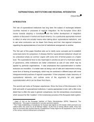
FIGURE 1<br />
1 000<br />
gfcf in Latin America, in constant dollars at 1950 prices<br />
(Index: 1950=100)<br />
100<br />
10<br />
1<br />
1856<br />
1860<br />
1864<br />
1868<br />
1872<br />
1876<br />
1880<br />
1884<br />
1888<br />
1892<br />
1896<br />
1900<br />
1904<br />
1908<br />
1912<br />
1916<br />
1920<br />
1924<br />
1928<br />
1932<br />
1936<br />
1940<br />
1944<br />
1948<br />
1952<br />
1956<br />
1960<br />
1964<br />
1968<br />
1972<br />
1976<br />
1980<br />
1984<br />
1988<br />
1992<br />
1996<br />
2000<br />
2004<br />
2008<br />
Source: prepared by the authors on the basis of the annex table.<br />
gfcf: gross fixed capital formation.<br />
Years<br />
Focusing on the way in which the long-term<br />
capitalization process unfolded in Latin America as a<br />
whole, figure 1 and tables 1 and 2 shed light on two<br />
particularly interesting factors. One is that the peak<br />
in investment activity did not occur during the second<br />
half of the twentieth century, as is usually thought,<br />
but rather in the second half of the nineteenth century.<br />
This is especially evident when investment activity is<br />
measured in per-capita terms. The growth rate for gfcf<br />
from 1856 to 1890 was not equalled at any point in the<br />
twentieth century. The second outstanding feature of<br />
aggregate investment trends is the marked degree of<br />
volatility seen in the 100 years leading up to 1950. Figure<br />
1 shows quite clearly how investment growth cycles<br />
and phases have smoothed out since then. In fact, this<br />
change in trend is so marked that it may be regarded as<br />
signalling the emergence of a different and less unstable<br />
investment pattern. 13<br />
Turning back to the first point: the data indicate that<br />
the slowdown in investment actually began before the<br />
outbreak of the First World War. The period between 1890<br />
and 1913 was one of slow growth, as capital formation<br />
was depressed for the entire decade following the Baring<br />
crisis, which set foreign investors back for years. In the<br />
following period (1913-1929), a moderate upswing in<br />
growth was cut short by the Great Depression. The<br />
period 1929-1950 was the least robust stage in the 150<br />
years covered by this analysis, along with 1980-2008;<br />
in fact, it was so sluggish that, in per capita terms, total<br />
output was completely flat (see table 2). This evidence<br />
strongly refutes the traditional historical narrative, in<br />
which investment was said to have jumped with the<br />
advent of the import-substitution industrialization model<br />
which followed the disruption caused by the Great<br />
Depression. 14 It would seem that the financial squeeze<br />
13 The fact that this change in investment trends coincides with the<br />
point in time when these estimates begin to be based on official figures<br />
would seem to be grounds for a strong suspicion that this changover<br />
in data sources may be the reason why the series for the years before<br />
1950 reflect a much greater degree of volatility than the post-1950<br />
series do. I have been unable to find any corroborating evidence for<br />
that suspicion, however.<br />
14 The traditional view is taken up, from a critical perspective, in the<br />
essays of Luis Bértola and Jeffrey Williamson, Stephen Haber and Richard<br />
Salvucci that have been published in Bulmer-Thomas, Coatsworth and<br />
Cortés Conde (2006). The analysis authored by José A. Ocampo (2004)<br />
could be said to set out –for now– the canonical position on this issue,<br />
according to which the industrialization process gathered a huge amount<br />
of momentum in the 1930s and during the Second World War while<br />
not radically changing the development pattern of Latin America that<br />
had been in place up to the crisis of 1929.<br />
Capital formation in Latin America: one and a half century<br />
of macroeconomic dynamics • Xavier Tafunell
14<br />
cepal review 109 • april 2013<br />
occasioned by the interruption of external capital inflows<br />
and the decline in the purchasing power of exports played<br />
a more important part than government action did in<br />
galvanizing investment.<br />
Another noteworthy and rather surprising feature of<br />
tables 1 and 2 are the differences between countries over a<br />
century of gfcf growth. The rates of capital accumulation<br />
do not correlate to relative levels of per capita income in<br />
1950, according to data published by Maddison (2007).<br />
Mexico, the Dominican Republic (only in absolute terms)<br />
and Colombia exhibit the highest rates of capitalization<br />
between 1856 and 1950, yet their per capita gdp was below<br />
the average for Latin America in 1950. Also surprising<br />
is the fact that Ecuador and Haiti —two very laggard<br />
economies— built up capital at the same rate as the region<br />
overall. 15 Something similar may be supposed to have<br />
happened in Central America: although the evolution<br />
of investment has not been estimated for 1929-1950, in<br />
1856-1929 it gained more ground than in Latin America<br />
overall. Conversely, some of the region’s more developed<br />
economies, such as Chile, capitalized at below-average<br />
rates. The trajectories for other countries coincide with what<br />
might be expected in relation to their degree of economic<br />
development. It comes as no surprise, then, that investment<br />
in Argentina progressed further and investment in Brazil<br />
less than the regional average. Incidentally, investment<br />
patterns over the century provide the best illustration of<br />
the way the major investment opportunities offered by<br />
the first wave of globalization contrasted with the limited<br />
possibilities available once the international economy<br />
began to disintegrate.<br />
What explanation can there be for the fact that<br />
national gfcf growth rates in 1856-1950 are so unrelated,<br />
in many cases, to relative per capita gdp around 1950?<br />
The unexpected figures in tables 1 and 2 seem to cast an<br />
ominous doubt on the consistency of the quantification,<br />
regardless that previous findings (Tafunell, 2007, 2009a<br />
and 2009b) confirm its reliability. The key to the paradox<br />
lies, basically, in the starting levels of investment. These<br />
were very uneven in the mid-nineteenth century, as we<br />
will see below. But first, a look is warranted at how<br />
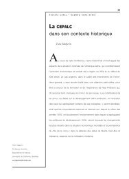
the two basic categories of investment (equipment and<br />
construction) evolved. These series are represented<br />
in figure 2. Tables 3 and 4 contain the figures for the<br />
average annual rates of variation for both categories in<br />
the periods under review.<br />
15 In these two cases, the growth rates do not refer to the total period<br />
because information is lacking for the first few years. But it is unlikely<br />
that the results would vary significantly if we had those data.<br />
In figure 2 it leaps to the eye that capital formation<br />
in machinery and related equipment climbed more<br />
vigorously than investment in construction (and more,<br />
obviously, than overall investment). This makes sense,<br />
since long-term economic growth depends more on<br />
the endowment and quality of machinery than on the<br />
acquisition and renewal of other capital goods. In<br />
Latin America, during the century prior to 1950, the<br />
difference between the two annual growth rates was quite<br />
considerable: 6.3%, compared with 4.6. 16 Interestingly,<br />
the difference between the two rates was greatest in the<br />
period 1856-1913 (8.5% and 5.9%, respectively), then<br />
it narrowed sharply in 1913-1950 (3.1% and 2.6 %,<br />
respectively). What is more, between 1929 and 1950, the<br />
relative positions shifted: capital formation in equipment<br />
rose very little, whereas investment in construction rose<br />
in keeping with its moderate growth since 1890. Figure<br />
2 shows very clearly that capital formation grew faster in<br />
equipment than in construction until 1890. Since then,<br />
the two series have followed a very similar long-term<br />
trajectory. All this backs up the idea mentioned earlier<br />
that the capitalization process in the second half of the<br />
nineteenth century was materially different to the process<br />
in the first half of the twentieth century.<br />
This is, undoubtedly, the most important lesson<br />
to be drawn from the comparison between tables 3 and<br />
4. The varied investment profiles of the growth phases<br />
between 1856 and 1950 are also interesting to examine.<br />
In the upsurge of 1856 to 1873, equipment stock was<br />
accumulated at an extraordinarily high —and never<br />
repeated— annual rate of 12.2%, almost double the rate<br />
for investment in construction. In the following phase<br />
(1873-1890) the frenetic pace of railway laying drove<br />
growth in construction investment ahead of still-dynamic<br />
investment in machinery. The financial crisis of 1890<br />
dealt a harsh blow to the transport sector, with lasting<br />
effects, while the equipment endowment rose from<br />
then until 1929 at a respectable annual rate of almost<br />
6%. From a general perspective, the data in table 4 are<br />
notably similar to those in table 1, owing to the heavy<br />
weight of construction investment in gfcf. 17<br />
16 For example, in Spain the rates of increase over this century-long<br />
period were, respectively, 3.3% and 2.5%, with an aggregate investment<br />
growth rate of 2.6% per year, according to series prepared by Prados<br />
de la Escosura (2003).<br />
17 It will be recalled that the index numbers series for the two categories<br />
of gfcf have been transformed by applying the magnitude of gfcf<br />
in 1950, at that year’s prices. At that date, investment in construction<br />
represented 63.8% of overall investment in Latin America (17 countries).<br />
It is worth adding that the differences between countries in this respect<br />
are not very significant, with a standard deviation of 8.8.<br />
Capital formation in Latin America: one and a half century<br />
of macroeconomic dynamics • Xavier Tafunell
cepal review 109 • april 2013<br />
15<br />
FIGURE 2<br />
300,0<br />
gfcf in Latin America, in constant dollars at 1950 prices<br />
(Index: 1929=100)<br />
30,0<br />
3,0<br />
0,3<br />
1856<br />
1858<br />
1860<br />
1862<br />
1864<br />
1866<br />
1868<br />
1870<br />
1872<br />
1874<br />
1876<br />
1878<br />
1880<br />
1882<br />
1884<br />
1886<br />
1888<br />
1890<br />
1892<br />
1894<br />
1896<br />
1898<br />
1900<br />
1902<br />
1904<br />
1906<br />
1908<br />
1910<br />
1912<br />
1914<br />
1916<br />
1918<br />
1920<br />
1922<br />
1924<br />
1926<br />
1928<br />
1930<br />
1932<br />
1934<br />
1936<br />
1938<br />
1940<br />
1942<br />
1944<br />
1946<br />
1948<br />
1950<br />
Equipment<br />
Years<br />
Construction<br />
Source: prepared by the author on the basis of the annex table.<br />
gfcf: gross fixed capital formation.<br />
TABLE 3<br />
Cumulative average annual growth rate of gross investment in equipment<br />
(Percentages)<br />
Period<br />
Argentina<br />
Bolivia<br />
Brazil<br />
Chile<br />
Colombia<br />
Costa Rica<br />
Cuba<br />
Ecuador<br />
El Salvador<br />
Haiti<br />
Honduras<br />
Mexico<br />
Nicaragua<br />
Peru<br />
Dominican<br />
Republic<br />
Uruguay<br />
Venezuela<br />
Central America<br />
Latin America<br />
(17 countries )<br />
1856-1950 8.4 ... 5.8 5.3 5.4 ... 4.5 a 7.3 b ... 5.0 a ... 7.8 ... 6.6 4.7 a 4.6 a 7.7 ... 6.3<br />
1856-1913 11.7 ... 8.9 7.9 5.9 ... ... ... ... ... ... 9.1 ... 6.7 ... ... 6.0 7.7 8.5<br />
1913-1950 3.4 -0.5 1.1 1.4 4.6 1.7 2.8 4.6 4.2 4.9 7.2 5.8 1.8 6.5 1.4 1.6 10.3 ... 3.1<br />
1856-1873 13.2 ... 12.0 11.0 13.4 ... ... ... ... ... ... 14.1 ... 19.0 ... ... 3.5 4.1 12.2<br />
1873-1890 19.5 ... 7.8 9.5 -1.1 ... 6.2 22.3 ... 9.1 ... 11.1 ... -5.0 20.4 9.5 10.1 15.9 8.5<br />
1890-1913 5.2 33.4 7.5 4.6 6.0 5.2 4.5 7.9 5.6 3.2 8.3 4.0 1.9 7.3 6.0 3.1 4.8 4.6 5.8<br />
1913-1929 6.1 3.8 1.8 6.4 12.6 6.1 0.9 6.1 4.7 7.5 5.8 6.4 5.4 4.8 0.9 5.6 12.8 5.8 5.1<br />
1929-1950 1.5 -3.6 0.6 -2.2 -1.1 -1.5 4.3 3.4 3.8 3.0 8.3 5.3 -0.9 7.7 7.8 -1.3 8.4 ... 1.7<br />
Source: prepared by the author on the basis of the annex table.<br />
a 1870-1950.<br />
b 1865-1950.<br />
Capital formation in Latin America: one and a half century<br />
of macroeconomic dynamics • Xavier Tafunell
16<br />
cepal review 109 • april 2013<br />
Table 4<br />
Cumulative average annual growth rate of gross investment in construction<br />
(Percentages)<br />
Period<br />
Argentina<br />
Bolivia<br />
Brazil<br />
Chile<br />
Colombia<br />
Costa Rica<br />
Cuba<br />
Ecuador<br />
El Salvador<br />
Haiti<br />
Honduras<br />
Mexico<br />
Nicaragua<br />
Peru<br />
Dominican<br />
Republic<br />
Uruguay<br />
Venezuela<br />
Central America<br />
Latin America<br />
(17 countries )<br />
1856-1950 5.3 ... 3.4 3.5 6.8 ... 4.5 a 5.1 b ... 5.2 a ... 6.4 ... 4.7 6.4 a 5.7 6.5 ... 4.6<br />
1856-1913 8.0 ... 4.1 4.9 6.1 ... ... ... ... ... ... 6.8 ... 4.3 ... 9.1 4.9 7.0 5.9<br />
1913-1950 1.3 1.2 2.3 1.2 7.9 3.3 0.0 4.9 4.0 2.3 4.2 5.8 5.5 5.4 4.6 0.6 9.0 ... 2.6<br />
1856-1873 9.8 ... 3.5 6.9 12.1 ... ... ... ... ... ... 4.5 ... 11.5 ... 13.2 10.2 7.7 6.4<br />
1873-1890 16.8 ... 3.4 9.9 0.6 ... 5.6 5.6 ... 5.0 ... 23.2 ... -3.1 12.5 7.8 6.8 12.5 11.3<br />
1890-1913 0.8 23.6 5.0 0.0 6.0 12.9 11.3 -3.0 0.8 9.2 18.8 -2.2 -5.5 4.8 1.2 7.1 -0.2 2.5 1.8<br />
1913-1929 5.1 34.3 0.8 2.2 7.5 11.3 16.8 0.6 -1.5 4.1 29.0 -2.9 -3.1 -2.6 1.4 6.1 -0.6 3.1 2.5<br />
1929-1950 1.9 1.3 3.9 0.0 5.7 0.9 -0.1 0.9 1.1 4.3 5.9 6.3 2.0 2.9 6.0 -3.5 4.4 ... 2.6<br />
Source: prepared by the author on the basis of the annex table.<br />
a 1870-1950.<br />
b 1865-1950.<br />
We now return to the questions that remained<br />
unanswered from the reading of tables 1 and 2. A working<br />
hypothesis may be formed on the basis of table 5. The<br />
first few rows of data speak of very uneven levels of<br />
investment per capita within the region around 1856.<br />
These levels were uneven later, too, in fact throughout<br />
the period under study. And it may be tempting to say that<br />
there have always been huge inequalities in this respect—<br />
as there are, indeed, in other economic aggregates. In<br />
colonial times, especially latterly, levels of production<br />
activity, and in all probability investment, are known to<br />
have differed greatly in the various territories, although<br />
these disparities were not necessarily exactly as shown<br />
in the first few rows of table 5. All the evidence available<br />
points to early development —around the middle third<br />
of the nineteenth century— in a few economies such as<br />
Cuba, Argentina, Chile and Uruguay (probably in that<br />
order), and to lag and stalled or very weak growth in that<br />
period in other economies such as Colombia, Ecuador,<br />
Bolivia, Mexico, Peru, Venezuela and the small Central<br />
American states, except for Costa Rica. 18<br />
What is really startling in table 5 are the gaping<br />
differences in the endowment of new capital per capita<br />
by the middle decades of the nineteenth century. Whereas<br />
18 Bértola and Ocampo (2010, p. 19) note that economic inequalities<br />
were very great in the period 1820-1870. They find that Argentina and<br />
Uruguay were the earliest developers, followed by Chile and Cuba.<br />
Argentina and Chile were investing around US$ 9 (at<br />
1950 prices) annually per capita, Mexico, the Central<br />
American nations, Peru and Colombia were investing<br />
US¢ 16, US¢ 45, US¢ 74 and US¢ 89, respectively.<br />
We now turn to the data for the 1870s, when economic<br />
globalization was beginning to inject vigour into the<br />
Latin American economies, and for which my data<br />
processing spans a larger and more representative group<br />
of nations. Taking the leading economy, Argentina, as<br />
a reference, we see that the investment effort in the<br />
next most prosperous economies (Chile and Uruguay)<br />
was around 50% and 75% of Argentina’s, as shown in<br />
table 5, 19 and 25% of that figure for Latin America as<br />
19 Cuba should also figure in this group, but the Ten Years’ War (1868-<br />
1878) depressed investment in the country. With regard to Uruguay, the<br />
data in the table and the annex require some clarification. My estimate<br />
for investment in construction yields figures too high to be credible<br />
until, at least, the final years of the nineteenth century. Fortunately,<br />
there is another measurement with which to compare and substitute<br />
mine: one prepared by Bértola (1998). This author calculated the<br />
gross value added of the construction industry on the basis of data on<br />
building permits and public works spending. Comparison of his series<br />
and mine shows that the two have a broadly similar profile in terms of<br />
cyclical movements, but diverge significantly as to level before 1900.<br />
For want of a better explanation, I assume that my figures grossly<br />
overstate the level of investment in Uruguay because much of the<br />
material imported through the port of Montevideo was in fact destined<br />
for the Argentine market. This is mere conjecture, however, and needs<br />
to be verified. Meanwhile, I have adopted the series constructed by<br />
Bértola and linked it with mine in 1870 and 1936.<br />
Capital formation in Latin America: one and a half century<br />
of macroeconomic dynamics • Xavier Tafunell
cepal review 109 • april 2013<br />
17<br />
TABLE 5<br />
gfcf per capita in dollars at constant 1950 prices<br />
(Ten-year averages)<br />
Period<br />
Argentina<br />
Bolivia<br />
Brazil<br />
Chile<br />
Colombia<br />
Costa Rica<br />
Cuba<br />
Ecuador a<br />
El Salvador<br />
Haiti<br />
Honduras<br />
Mexico<br />
Nicaragua<br />
Peru<br />
Dominican<br />
Republic<br />
Uruguay<br />
Venezuela<br />
Central America<br />
Latin America<br />
(17 countries)<br />
1856-1859 9.3 ... 6.1 9.3 0.9 ... ... ... ... ... ... 0.2 ... 0.7 ... ... 2.0 0.5 3.0<br />
1860-1869 22.1 ... 6.3 13.6 3.4 ... ... 0.3 ... ... ... 0.6 ... 1.2 ... ... 3.1 0.6 4.9<br />
1870-1879 35.5 ... 11.8 17.7 5.3 ... 7.6 0.9 ... 0.7 ... 1.0 ... 4.4 3.6 27.0 4.1 2.1 8.8<br />
1880-1889 120.0 ... 13.6 24.2 8.2 ... 8.8 2.6 ... 0.8 ... 3.4 ... 1.1 9.0 56.8 14.4 5.3 18.1<br />
1890-1899 82.0 0.1 16.9 34.6 5.8 20.8 19.8 3.1 5.7 2.6 0.7 6.4 4.3 1.6 10.8 35.0 10.2 9.4 17.9<br />
1900-1909 94.6 0.9 13.9 43.1 4.6 28.4 33.1 3.2 2.2 1.3 1.2 8.8 2.5 2.8 4.0 55.4 4.5 6.2 19.7<br />
1910-1919 90.7 1.3 18.7 50.6 9.5 25.7 56.5 3.4 4.8 3.8 5.6 6.3 4.0 3.2 13.1 91.9 10.9 8.4 24.4<br />
1920-1929 92.6 2.5 21.9 64.5 36.9 42.6 55.2 8.7 12.2 4.0 9.9 11.7 7.4 7.4 19.4 204.4 70.2 17.3 33.9<br />
1930-1939 96.3 2.2 17.1 49.6 27.8 53.7 14.1 6.4 7.0 2.7 8.4 12.1 4.7 6.7 7.1 167.8 100.8 ... 31.4<br />
1940-1950 106.4 3.0 25.4 60.3 45.5 57.3 25.4 8.4 10.4 4.7 12.8 24.2 7.5 15.3 12.5 91.8 233.2 ... 42.8<br />
Source: X. Tafunell, “Un siglo de formación de capital en América Latina (1856-1950). Ensayo de cuantificación general”, paper presented at<br />
the X International Congress of the Spanish Association of Economic History (Carmona, Spain, 7-9 September), 2011.<br />
a The figure shown for 1860-1869 is the average for 1865-1869.<br />
gfcf: gross fixed capital formation.<br />
a group. The most laggard economies show investment<br />
efforts of less than 10% of the figure for Argentina: 8.1%<br />
for the Dominican Republic; 6% for the small Central<br />
American states; 2.9% for Mexico; 2.6% for Ecuador;<br />
and 1.8% for Haiti. Ahead of this group of severely<br />
undercapitalized economies was another group, with<br />
investment levels that were still very low, comprising<br />
Colombia (15.1% of Argentina’s level), Peru (12.7%)<br />
and Venezuela (11.5%).<br />
What emerges from table 5, then, is that the<br />
economies that were the region’s richest at the end of<br />
the first globalization period (Argentina, Uruguay, Chile<br />
and Cuba) made headway in capital formation very early<br />
on. In the middle decades of the nineteenth century, if<br />
not before, these countries enjoyed an investment boom<br />
as a result of which their per capita investment levels<br />
were, fluctuations notwithstanding, several times those<br />
of poor economies by the starting point of the series<br />
(1856-1859). It follows, then, that great divergence<br />
must have occurred within the region in the first half<br />
of the nineteenth century. This being so, the more<br />
laggard economies, whose levels of capitalization per<br />
capita were tiny around 1850, would naturally tend to<br />
capitalize faster than the advanced economies whenever<br />
the opportunity arose, as is apparent in table 2. This,<br />
of course, produced a certain amount of convergence<br />
within the region, at least in terms of capital formation.<br />
In an earlier work (Tafunell, 2009a), I postulated this<br />
hypothesis for the period 1914-1930. 20 Now, the data<br />
processing over a much longer period seems to bear out<br />
that hypothesis for the century and a half since 1856.<br />
A more careful analysis of the series, beyond this rapid<br />
presentation of the qualitative reconstruction performed,<br />
would test this hypothesis and its validity for different<br />
historical subperiods.<br />
20 Bértola and Ocampo (2010, pp. 19-20 and 26) argue that there was<br />
a process of economic convergence in the region from 1910 to 1990.<br />
Capital formation in Latin America: one and a half century<br />
of macroeconomic dynamics • Xavier Tafunell
18<br />
cepal review 109 • april 2013<br />
IV<br />
Fluctuations in gfcf: cycles and volatility<br />
Figure 1 shows a markedly cyclical dynamic. Shortterm<br />
movements (of no more than a decade) prevail<br />
over long-term growth trends of the aggregate. The<br />
cyclical fluctuations over the course of several historical<br />
intervals are large enough and sharp enough to eclipse<br />
underlying trends.<br />
The cyclical peaks depicted in figure 1 are compiled<br />
in table 6, which shows the cumulative average annual<br />
growth rate recorded in each of these cycles —from high<br />
to high— and a simple measure of investment volatility,<br />
the standard deviation of the year-on-year variation rates.<br />
TABLE 6<br />
Period<br />
gfcf cycles in Latin America<br />
Average annual<br />
rate of growth<br />
(percentages)<br />
Standard deviation<br />
of year-on-year<br />
variation rates<br />
1856-1860 5.9 13.7<br />
1860-1865 11.5 16.1<br />
1865-1874 7.9 19.2<br />
1874-1884 7.5 16.4<br />
1884-1890 14.6 27.7<br />
1890-1896 -9.1 29.5<br />
1896-1907 6.6 22.9<br />
1907-1913 6.7 9.8<br />
1913-1920 -5.9 44.6<br />
1920-1929 11.6 23.5<br />
1929-1937 -1.1 28.4<br />
1937-1947 6.9 25.4<br />
1947-1949 -2.8 21.6<br />
1949-1952 5.4 9.6<br />
1952-1958 4.6 3.7<br />
1958-1962 4.1 4.6<br />
1962-1980 7.2 3.5<br />
1980-1987 -2.8 9.0<br />
1987-1994 3.1 4.5<br />
1994-1998 4.1 7.0<br />
1998-2000 -1.0 5.1<br />
2000-2008 5.7 7.0<br />
1856-1950 4.9 25.3<br />
1950-2008 4.4 6.8<br />
1856-2008 4.7 20.4<br />
Source: prepared by the author on the basis of the annex table and<br />
http://www.cepal.org/deype/cuaderno37/esp/index.htm.<br />
gfcf: gross fixed capital formation.<br />
Leaving aside the well-known events since the<br />
Second World War, a first point which merits attention<br />
is that there were only three episodes of slippage: 1890-<br />
1896, 1913-1920 and 1929-1937.<br />
In the first of these cycles the fall was very sharp:<br />
almost half (43.7%) measured from high to high. The<br />
data show, then, that the Baring crisis had a deeply<br />
depressive effect that set it apart from other crises, as<br />
several authors have argued (Mitchener and Weidenmier,<br />
2008). The plunge caused by the First World War was not<br />
as deep, thanks to the powerful reactivation that ensued<br />
in 1919-1920. In the last of the three cycles (1929-1937)<br />
the contraction endured during the fateful years of the<br />
Great Depression weighed more heavily than the upturn<br />
generated by the kick-start of industrialization by import<br />
substitution. A final interesting point in this connection<br />
is that capitalization slumped more heavily in the two<br />
great depressions mentioned than in the “lost decade”<br />
of the 1980s.<br />
Turning to cycles dominated by the upswing,<br />
the first observations is that these predominate<br />
overwhelmingly: high positive average annual rates of<br />
variation characterized 9 of the 12 cyclical movements<br />
identified. The cycles with the largest overall increases<br />
measured from peak to peak were 1884-1890, 1860-1865<br />
and 1920-1929. The first stands out significantly from<br />
the others. The other two were similar, but given that the<br />
last doubled the first in length, it may be said that the<br />
two largest cyclical investment drives in pre-1950 Latin<br />
America occurred in the 1880s and the 1920s. This is<br />
consistent with the fact that the contractions that ended<br />
these booms were the severest in the century between<br />
1856 and 1950, except for the downturn during the<br />
First World War. Obviously, the latter was exceptional<br />
inasmuch as its cause was wholly exogenous, unlike other<br />
investment crises. What is more, all the cycles —except<br />
those indicated— were characterized by a relatively high<br />
and stable rate of investment growth: between 6% and<br />
8% per year. This was, according to the data, the cruising<br />
speed at which Latin America managed to capitalize<br />
until the Second World War. The region departed from<br />
this investment pattern —with either positive or negative<br />
variations— only during a few periods of turbulence in<br />
extraordinary circumstances. Since the Second World<br />
War, the stationary rate of investment has been lower,<br />
from 4% to 5% per year. The most obvious deviation<br />
Capital formation in Latin America: one and a half century<br />
of macroeconomic dynamics • Xavier Tafunell
cepal review 109 • april 2013<br />
19<br />
from this cyclical pattern occurred towards the end<br />
of the “golden age” (1962-1980), during which Latin<br />
America exhibited the most sustained, though not the<br />
most intensive, investment effort in its history.<br />
For reasons of space, it is outside the scope of this<br />
work to analyse the nature of the movements in the series<br />
in greater depth. Yet there is one highly idiosyncratic<br />
component of the macromagnitude examined which<br />
should not be overlooked: its great variability. The data<br />
in table 6 show clearly that investment has fluctuated<br />
strongly. The measure of volatility far exceeded the<br />
annual growth rate in all the cycles. The only two<br />
exceptions to this pattern occurred at the time of the<br />
largest boom, during the shield of State intervention<br />
(from 1952 to 1958 and from 1962 to 1980). But the<br />
prime focus of attention must be the fact that in the<br />
century prior to 1950, standard deviation was five<br />
times the rate of annual variation, which speaks of an<br />
extremely volatile variable. By contrast, since 1950<br />
the investment cycle has become much less extreme<br />
(standard deviation is only 50% more than the growth<br />
rate). The most severe cycle by far was during the First<br />
World War, when there was an extreme swing between<br />
the most violent contractionary and expansionary phases<br />
in the last century and a half. The cycles of 1884-1890,<br />
1890-1896 and 1929-1937 were also turbulent, with<br />
large expansions and reactivations before and after<br />
major slumps. Conversely, the expansionary cycle at the<br />
end of the belle époque (1907-1913) was characterized<br />
by a very stable rate of growth. No doubt the mythical<br />
aura surrounding this period has much to do with that<br />
regularity. Interestingly, the same cannot be said of the<br />
other period often thought to be the most prosperous<br />
before the “golden age”: the 1920s.<br />
V<br />
Concluding remarks<br />
Empirical studies on the theory of economic growth<br />
are limited by a lack of statistical data on the basic<br />
macromagnitudes of developing economies in the<br />
period before 1950. In the case of the Latin American<br />
countries, data on capital formation were particularly<br />
lacking. This work has to a great extent covered that<br />
deficit by providing a quantification of gfcf and its<br />
two main components —investment in equipment and<br />
in construction— for all the countries of the region,<br />
except Guatemala, Panama and Paraguay. The annual and<br />
continuous series provided span the period from 1856 to<br />
1950. Linking these series with those generated by the<br />
official national accounts systematized and standardized<br />
by eclac provides a reliable quantification of gfcf in<br />
the Latin American economies from 1856 to the present.<br />
Several important facts emerge from the examination<br />
of very long-term gfcf patterns. First, the greatest<br />
investment growth occurred in the second half of the<br />
nineteenth century, during the first wave of globalization;<br />
more specifically, between 1856 (possibly earlier) and<br />
1890. Second, it was over this period, not later, that<br />
equipment endowment grew faster than endowments<br />
of other capital goods, which means that the region’s<br />
economies boosted their long-term growth potential more<br />
in the nineteenth century than they did later, or at least<br />
during the first half of the twentieth century. Third, gfcf<br />
was highly volatile during the century leading up to 1950,<br />
becoming much less so thereafter. The explanation for the<br />
contrast probably lies in the key impact of primary goods<br />
exports and foreign capital on gfcf before the Second<br />
World War. Insofar as investment instability is bad for<br />
economic growth, the possibilities for Latin American<br />
economies have brightened since the Second World War.<br />
Fourth and last, the data show that the most laggard<br />
economies have tended to make a greater investment<br />
effort per capita than more advanced economies. This<br />
has produced only very partial convergence, however:<br />
the disparities in per capita investment levels, which were<br />
extreme in the mid-nineteenth century, have remained<br />
very sharp.<br />
Capital formation in Latin America: one and a half century<br />
of macroeconomic dynamics • Xavier Tafunell
20<br />
cepal review 109 • april 2013<br />
ANNEX<br />
Table A-1<br />
Gross fixed capital formation (gfcf) at constant prices<br />
(Index: 1929=100 )<br />
Year Argentina<br />
Bolivia<br />
(Plurinational State of)<br />
Brazil Chile Colombia Costa Rica Cuba Ecuador<br />
Equipment<br />
Construction<br />
gfcf<br />
Equipment<br />
Construction<br />
gfcf<br />
Equipment<br />
Construction<br />
gfcf<br />
Equipment<br />
Construction<br />
gfcf<br />
Equipment<br />
Construction<br />
gfcf<br />
Equipment<br />
Construction<br />
gfcf<br />
Equipment<br />
Construction<br />
gfcf<br />
Equipment<br />
Construction<br />
gfcf<br />
1856 0.1 1.1 0.8 0.6 10.0 4.9 0.5 4.1 2.0 0.6 0.6 0.6<br />
1857 0.1 1.0 0.7 1.3 8.3 4.5 0.7 4.7 2.4 0.2 0.6 0.3<br />
1858 0.0 0.7 0.5 1.5 8.0 4.5 0.9 6.8 3.4 0.4 0.5 0.4<br />
1859 0.1 1.0 0.7 1.5 7.8 4.4 0.6 6.1 2.9 0.6 0.4 0.5<br />
1860 0.1 1.0 0.7 1.7 12.2 6.5 0.7 7.8 3.7 0.4 0.5 0.5<br />
1861 0.1 0.9 0.7 1.7 10.3 5.6 1.0 9.4 4.5 1.7 0.6 1.3<br />
1862 0.1 1.0 0.8 2.1 8.9 5.2 0.3 6.3 2.8 1.2 0.9 1.1<br />
1863 0.2 2.7 2.0 1.9 7.3 4.4 0.9 5.2 2.7 1.6 1.8 1.7<br />
1864 0.2 3.8 2.7 1.1 10.4 5.4 1.9 5.9 3.6 2.1 2.8 2.4<br />
1865 0.5 5.1 3.7 1.9 8.8 5.0 1.3 11.2 5.4 1.5 1.6 1.5 0.9 1.8 1.5<br />
1866 0.4 3.7 2.7 1.7 6.7 4.0 1.4 5.4 3.0 2.8 2.3 2.6 1.1 0.6 0.7<br />
1867 0.3 2.0 1.5 1.5 8.7 4.8 2.7 8.0 4.9 3.6 3.0 3.4 0.3 1.7 1.2<br />
1868 0.3 2.5 1.8 2.0 9.1 5.2 2.6 8.8 5.2 2.4 3.2 2.7 0.0 1.6 1.0<br />
1869 0.4 5.1 3.7 2.6 11.1 6.5 2.6 15.9 8.2 2.5 2.2 2.4 1.1 1.9 1.6<br />
1870 0.6 5.2 3.8 3.0 10.4 6.4 2.0 20.9 9.9 2.8 3.6 3.0 7.2 2.8 4.5 0.7 1.8 1.5<br />
1871 0.3 7.5 5.4 2.9 20.1 10.7 1.8 14.4 7.1 3.9 2.6 3.4 9.8 1.5 4.6 6.1 4.1 4.8<br />
1872 0.7 5.2 3.8 3.2 20.6 11.2 2.2 12.6 6.5 5.4 5.7 5.5 12.6 2.3 6.2 2.6 4.1 3.5<br />
1873 0.6 5.5 4.1 3.9 18.0 10.4 2.8 12.6 6.9 4.7 4.5 4.7 11.4 3.2 6.3 0.2 16.8 11.0<br />
1874 0.9 10.6 7.7 3.9 19.1 10.9 2.5 21.5 10.4 3.6 2.2 3.1 8.1 3.8 5.4 1.0 5.6 4.0<br />
1875 0.6 7.7 5.6 4.0 15.9 9.4 2.5 18.1 9.0 2.7 1.4 2.2 7.6 3.3 4.9 0.2 1.8 1.2<br />
1876 0.3 4.3 3.1 3.7 19.5 10.9 2.3 9.1 5.2 3.0 1.1 2.3 7.4 2.9 4.6 2.0 3.4 2.9<br />
1877 0.2 2.8 2.0 3.1 30.8 15.8 1.1 6.5 3.3 3.6 1.3 2.8 8.6 12.2 10.8 7.8 2.6 4.4<br />
1878 0.4 3.1 2.3 3.7 28.3 15.0 0.9 8.3 4.0 3.8 2.1 3.2 10.4 18.8 15.6 2.0 2.2 2.1<br />
1879 0.4 4.9 3.6 3.5 32.7 16.8 0.8 6.4 3.1 3.8 4.8 4.2 10.4 10.9 10.7 1.1 3.0 2.3<br />
1880 0.4 5.2 3.8 5.3 22.7 13.2 0.8 12.0 5.5 4.6 3.7 4.3 9.0 4.6 6.2 3.2 6.7 5.4<br />
1881 0.8 7.3 5.4 6.0 31.4 17.6 1.5 12.7 6.2 4.7 2.6 3.9 11.2 4.3 6.9 4.6 8.4 7.1<br />
1882 1.6 19.1 13.9 7.1 35.1 19.9 2.2 18.4 8.9 6.8 5.7 6.4 17.2 4.1 9.0 3.8 8.9 7.1<br />
1883 2.6 29.1 21.3 8.9 30.2 18.6 3.7 19.7 10.4 8.7 8.4 8.6 21.0 6.7 12.1 1.7 2.5 2.2<br />
1884 4.9 32.8 24.6 9.4 29.3 18.5 4.5 25.5 13.2 6.6 14.2 9.4 14.5 7.0 9.8 3.7 10.7 8.2<br />
1885 3.9 21.8 16.5 7.8 21.2 13.9 1.8 16.3 7.9 4.7 9.6 6.5 10.7 5.8 7.6 4.8 4.5 4.6<br />
1886 3.5 19.8 15.0 8.0 20.8 13.9 1.9 19.0 9.0 5.8 5.2 5.6 14.4 6.1 9.2 10.1 12.4 11.6<br />
1887 4.7 22.1 17.0 8.3 16.3 11.9 2.8 23.0 11.2 5.2 7.9 6.2 13.3 5.4 8.4 14.9 24.0 20.8<br />
1888 8.1 54.6 40.9 9.6 22.0 15.3 3.6 24.9 12.5 4.2 4.7 4.4 16.9 6.0 10.1 13.7 50.0 37.2<br />
1889 11.4 60.4 46.0 10.1 28.5 18.5 10.5 36.6 21.4 3.9 7.2 5.1 25.8 8.3 14.9 8.6 24.8 19.1<br />
1890 12.0 76.9 57.8 0.1 0.6 0.3 14.2 31.7 22.2 13.3 63.2 34.1 3.9 5.0 4.3 11.9 2.3 7.7 31.5 8.2 17.0 6.7 42.6 30.0<br />
1891 5.3 25.8 19.8 0.4 0.3 0.4 32.1 37.6 34.6 7.4 31.8 17.6 4.0 5.6 4.6 13.2 4.6 9.4 40.3 7.3 19.7 9.1 20.4 16.4<br />
1892 3.8 8.2 6.9 2.2 0.6 1.6 24.7 25.7 25.2 11.9 32.7 20.6 3.8 4.4 4.0 11.8 7.0 9.7 49.2 27.2 35.4 7.5 10.4 9.4<br />
1893 6.1 10.1 8.9 0.4 1.2 0.7 25.9 22.9 24.5 9.4 24.3 15.6 4.0 6.5 4.9 8.5 9.1 8.7 42.8 48.6 46.4 8.7 9.7 9.3<br />
1894 5.2 8.8 7.7 0.9 1.2 1.0 19.3 16.5 18.0 10.2 36.3 21.1 3.2 4.9 3.8 8.2 16.5 11.9 33.7 30.3 31.6 10.2 10.4 10.4<br />
1895 4.5 13.4 10.8 0.3 0.5 0.4 24.8 37.4 30.6 10.9 35.6 21.2 3.4 4.9 4.0 10.4 6.4 8.6 17.9 6.1 10.5 7.9 17.9 14.4<br />
1896 4.4 30.2 22.6 0.4 0.5 0.4 24.8 43.0 33.1 7.9 25.0 15.0 4.8 6.6 5.4 12.4 16.8 14.3 6.4 5.1 5.6 10.5 27.4 21.4<br />
1897 4.3 19.6 15.1 1.2 0.3 0.8 16.7 28.0 21.9 4.7 8.3 6.2 5.4 9.0 6.7 11.6 23.5 16.9 3.8 7.4 6.0 11.8 17.8 15.7<br />
Capital formation in Latin America: one and a half century<br />
of macroeconomic dynamics • Xavier Tafunell
cepal review 109 • april 2013<br />
21<br />
Year Argentina<br />
Bolivia<br />
(Plurinational State of)<br />
Brazil Chile Colombia Costa Rica Cuba Ecuador<br />
1898 6.3 20.5 16.3 1.0 0.1 0.7 12.0 27.1 18.9 4.4 8.6 6.2 4.7 9.3 6.4 13.3 14.2 13.7 5.9 22.4 16.2 15.1 15.5 15.3<br />
1899 7.1 12.9 11.2 24.3 0.7 15.4 11.2 21.1 15.7 6.9 18.4 11.7 2.6 5.4 3.6 14.2 26.6 19.7 15.8 48.6 36.3 16.3 17.7 17.2<br />
1900 7.8 13.6 11.9 10.4 0.3 6.6 14.0 13.9 13.9 9.8 10.8 10.2 1.5 0.9 1.3 17.7 11.6 15.0 22.2 22.1 22.1 24.2 13.4 17.2<br />
1901 8.9 18.1 15.4 32.0 0.6 20.2 8.6 10.3 9.4 16.6 15.4 16.1 2.8 1.9 2.5 15.9 14.7 15.4 34.3 31.6 32.6 30.5 21.4 24.6<br />
1902 8.1 13.0 11.5 38.0 0.3 23.9 11.0 14.1 12.4 8.9 11.4 9.9 4.0 1.2 3.0 16.6 17.7 17.1 24.5 30.8 28.4 17.9 4.6 9.3<br />
1903 11.0 15.7 14.3 12.7 0.3 8.1 12.5 13.7 13.0 10.8 12.3 11.5 6.7 1.3 4.7 22.6 9.5 16.8 26.2 24.6 25.2 17.7 5.3 9.7<br />
1904 19.0 22.1 21.2 13.3 2.8 9.4 16.4 18.0 17.1 19.3 16.8 18.3 5.4 2.2 4.3 21.1 12.6 17.4 42.0 31.4 35.4 23.1 12.9 16.4<br />
1905 28.4 34.7 32.9 19.6 2.2 13.1 23.0 26.6 24.7 28.7 27.2 28.0 5.5 3.1 4.7 20.9 13.9 17.8 77.3 53.6 62.5 31.2 26.3 28.0<br />
1906 40.8 53.8 50.0 13.1 8.9 11.5 30.5 44.2 36.8 43.4 32.2 38.7 4.6 4.4 4.5 30.6 22.9 27.2 70.4 57.3 62.2 28.8 21.5 24.1<br />
1907 38.4 59.7 53.4 29.1 11.6 22.5 41.2 45.7 43.3 47.3 44.4 46.1 6.6 4.1 5.7 36.2 19.7 28.9 62.3 63.4 63.0 26.6 13.3 18.0<br />
1908 32.1 50.6 45.2 23.8 15.1 20.5 41.3 47.4 44.1 42.2 29.1 36.7 7.4 4.5 6.3 31.2 20.2 26.3 45.2 62.5 56.0 25.5 15.7 19.2<br />
1909 38.6 73.8 63.4 19.0 11.6 16.2 42.8 53.2 47.6 18.7 42.6 28.6 7.4 8.2 7.7 27.1 31.2 28.9 50.8 64.2 59.2 27.9 23.1 24.8<br />
1910 46.1 76.0 67.2 18.4 19.8 18.9 52.9 60.5 56.4 21.3 45.3 31.3 9.5 8.7 9.2 28.1 34.1 30.8 77.2 75.0 75.8 27.6 20.4 23.0<br />
1911 39.0 77.5 66.2 22.7 26.5 24.1 61.8 63.6 62.6 33.5 60.7 44.9 11.1 10.3 10.8 35.2 41.6 38.0 85.8 84.8 85.2 33.9 20.2 25.0<br />
1912 40.1 69.7 61.0 32.2 23.7 29.0 84.4 86.8 85.5 38.2 68.1 50.7 11.9 13.1 12.4 36.8 36.0 36.5 84.9 90.6 88.4 33.5 22.9 26.6<br />
1913 38.8 91.7 76.1 54.9 83.1 65.4 74.8 98.2 85.5 37.2 63.8 48.2 15.0 19.0 16.4 38.6 37.0 37.9 86.9 96.8 93.1 39.0 20.9 27.3<br />
1914 24.4 57.4 47.7 26.7 33.0 29.0 33.9 42.7 37.9 25.1 44.7 33.2 13.9 17.7 15.3 25.7 25.4 25.5 68.5 87.6 80.4 35.5 22.4 27.0<br />
1915 11.5 27.2 22.6 10.1 12.4 11.0 11.1 21.1 15.7 6.8 23.0 13.6 9.4 11.3 10.1 15.2 12.8 14.1 90.6 92.6 91.9 21.6 24.9 23.7<br />
1916 8.7 19.6 16.4 10.8 8.4 9.9 13.5 19.6 16.3 12.6 33.3 21.2 7.6 13.6 9.8 13.3 11.9 12.7 145.7 128.9 135.2 18.6 20.3 19.7<br />
1917 7.1 13.8 11.8 14.4 11.5 13.3 14.2 13.5 13.9 14.4 37.7 24.1 7.7 12.8 9.6 7.9 8.2 8.0 155.3 129.3 139.1 22.9 13.6 16.9<br />
1918 6.8 6.4 6.5 21.9 16.6 19.9 11.1 7.8 9.6 19.4 30.5 24.1 5.6 6.2 5.8 6.5 1.0 4.0 117.9 85.9 97.9 18.5 12.6 14.7<br />
1919 11.8 16.9 15.4 25.9 15.2 21.9 23.5 30.0 26.5 17.0 30.7 22.7 8.5 15.3 10.9 9.0 6.1 7.7 139.8 111.9 122.4 33.3 16.2 22.2<br />
1920 23.5 32.6 30.0 26.8 27.2 27.0 44.3 46.1 45.1 19.9 30.2 24.2 27.0 30.6 28.3 26.4 14.4 21.1 335.3 185.0 241.5 48.2 26.0 33.8<br />
1921 31.3 33.4 32.8 48.9 20.1 38.1 40.6 31.5 36.4 26.7 33.1 29.4 29.4 22.8 27.0 37.8 10.5 25.7 230.6 92.7 144.5 41.1 25.2 30.8<br />
1922 35.1 41.9 39.9 32.1 17.9 26.8 38.1 48.1 42.7 33.5 30.6 32.3 21.5 27.3 23.6 21.5 16.2 19.1 72.2 83.0 79.0 59.4 31.3 41.2<br />
1923 34.9 27.8 29.9 49.4 29.0 41.8 34.9 30.2 32.8 36.1 31.5 34.2 31.1 30.2 30.8 30.4 20.0 25.8 138.9 125.3 130.4 61.9 52.3 55.7<br />
1924 41.2 40.8 40.9 54.0 38.8 48.3 54.9 43.3 49.6 38.1 41.2 39.4 36.5 38.3 37.1 46.2 28.5 38.4 185.1 132.8 152.5 72.1 65.7 68.0<br />
1925 52.4 61.0 58.5 63.2 67.9 64.9 79.5 59.1 70.2 44.4 41.9 43.4 54.3 45.4 51.1 49.9 30.4 41.3 189.2 91.8 128.4 61.9 75.6 70.7<br />
1926 53.7 63.6 60.7 62.7 61.5 62.3 68.8 73.6 71.0 66.1 46.4 57.9 85.9 63.7 77.9 43.4 32.9 38.8 123.2 77.1 94.4 57.6 54.8 55.8<br />
1927 65.7 76.4 73.3 64.1 79.5 69.9 83.5 80.4 82.1 47.9 55.1 50.9 111.6 64.3 94.5 54.9 54.2 54.6 143.6 87.8 108.8 72.1 100.7 90.7<br />
1928 87.9 94.8 92.8 74.8 98.0 83.5 89.1 90.1 89.5 42.8 64.6 51.9 112.3 106.3 110.2 73.9 74.2 74.1 93.1 89.6 90.9 91.4 97.1 95.1<br />
1929 100.0 100.0 100.0 100.0 100.0 100.0 100.0 100.0 100.0 100.0 100.0 100.0 100.0 100.0 100.0 100.0 100.0 100.0 100.0 100.0 100.0 100.0 100.0 100.0<br />
1930 88.0 93.6 91.9 71.9 70.1 71.3 37.8 61.5 48.6 80.7 112.6 94.0 41.4 55.2 46.4 38.8 50.2 43.8 67.7 61.0 63.5 67.3 83.0 77.5<br />
1931 53.9 59.5 57.9 30.4 33.6 31.6 20.8 30.6 25.3 38.7 39.6 39.1 17.9 30.9 22.6 25.4 52.9 37.5 38.7 17.0 25.2 32.7 60.5 50.7<br />
1932 22.6 41.6 36.0 25.6 30.4 27.4 12.8 36.4 23.6 4.8 17.2 10.0 11.6 33.8 19.6 10.8 35.6 21.7 24.3 10.7 15.8 17.6 29.4 25.2<br />
1933 26.2 44.8 39.4 31.7 27.2 30.0 22.1 51.1 35.3 4.2 24.2 12.6 16.0 53.1 29.4 33.0 45.1 38.3 21.2 11.0 14.9 26.8 36.9 33.3<br />
1934 47.1 58.0 54.8 39.1 36.4 38.1 39.7 68.9 53.0 12.0 36.2 22.1 21.0 75.1 40.5 24.4 69.8 44.4 50.6 14.7 28.2 38.3 36.8 37.3<br />
1935 65.0 65.2 65.1 35.2 44.6 38.7 88.4 74.8 82.2 29.4 62.6 43.2 25.9 75.6 43.9 26.9 78.1 49.6 72.2 23.6 41.9 62.7 51.5 55.4<br />
1936 83.9 73.9 76.8 47.5 82.1 60.5 63.5 84.9 73.2 33.3 56.6 43.0 25.3 114.4 57.5 40.4 133.4 81.5 89.4 34.7 55.2 83.5 48.7 61.0<br />
1937 117.6 105.2 108.8 65.3 128.0 88.8 82.0 105.2 92.6 31.5 66.0 45.8 35.6 142.8 74.4 54.1 94.6 72.0 114.7 39.1 67.5 90.0 66.7 74.9<br />
1938 128.1 94.9 104.7 75.9 119.2 92.1 74.1 93.6 83.0 39.3 72.4 53.1 34.4 193.0 91.7 104.5 92.9 99.4 79.2 32.1 49.8 75.2 68.4 70.8<br />
1939 82.3 87.3 85.9 68.9 105.7 82.7 55.1 103.6 77.2 31.3 64.2 45.0 38.9 170.0 86.3 187.2 185.0 186.2 69.7 36.9 49.2 77.2 58.0 64.8<br />
1940 73.2 79.1 77.4 72.4 97.3 81.7 58.7 106.2 80.4 36.6 74.1 52.2 30.6 151.1 74.2 148.7 158.6 153.1 57.4 38.5 45.6 75.0 69.9 71.7<br />
1941 58.9 62.7 61.6 65.1 113.4 83.2 50.8 103.9 75.1 35.4 66.3 48.3 27.5 135.3 66.5 85.8 134.1 107.2 72.4 40.5 52.5 69.3 48.7 56.0<br />
1942 53.4 47.2 49.0 61.4 109.7 79.5 25.7 93.5 56.7 22.4 61.3 38.6 10.7 60.4 28.7 27.0 53.1 38.5 45.0 20.6 29.8 74.3 49.3 58.1<br />
1943 48.6 38.9 41.7 71.6 112.3 86.8 29.3 97.8 60.6 17.3 64.1 36.8 10.7 109.5 46.4 52.7 55.9 54.1 48.6 29.7 36.8 45.6 43.7 44.4<br />
1944 49.3 52.7 51.7 59.8 112.4 79.5 35.6 126.2 77.0 24.1 69.7 43.1 16.2 211.2 86.7 45.6 48.9 47.1 67.1 42.9 52.0 68.5 72.2 70.9<br />
1945 53.4 55.7 55.0 47.3 102.1 67.8 79.7 132.1 103.6 25.0 81.1 48.4 42.5 211.6 103.7 65.5 88.3 75.6 92.3 62.2 73.6 86.6 66.5 73.6<br />
1946 108.3 85.0 91.8 65.3 102.5 79.2 127.2 167.8 145.7 46.6 96.9 67.6 45.8 275.2 128.8 96.2 129.2 110.8 147.8 71.7 100.3 166.6 82.4 112.1<br />
1947 295.2 112.4 166.2 69.6 107.4 83.8 175.3 179.4 177.2 73.7 101.8 85.4 100.0 341.2 187.2 137.4 147.8 142.0 288.3 91.3 165.4 181.6 94.4 125.1<br />
1948 303.1 123.0 176.0 84.3 111.9 94.6 106.7 163.2 132.5 61.9 95.0 75.7 80.1 232.5 135.2 74.3 76.3 75.2 262.6 81.3 149.5 192.7 96.6 130.5<br />
1949 168.2 140.0 148.3 89.0 182.6 124.0 113.5 199.7 152.8 88.1 106.0 95.5 64.2 289.2 145.5 69.7 91.5 79.3 216.9 97.6 142.5 215.1 123.6 155.8<br />
1950 138.1 148.9 145.7 46.3 130.6 77.9 112.8 223.9 163.5 62.4 99.0 77.7 79.5 318.2 165.8 72.4 121.1 93.9 244.0 96.9 152.2 203.2 121.9 150.5<br />
Capital formation in Latin America: one and a half century<br />
of macroeconomic dynamics • Xavier Tafunell
22<br />
cepal review 109 • april 2013<br />
Table A-1 (continued)<br />
Gross fixed capital formation (gfcf) at constant prices<br />
(Index: 1929=100 )<br />
Year El Salvador Haiti Honduras Mexico Nicaragua Peru Dominican Republic Uruguay<br />
Equipment<br />
Construction<br />
gfcf<br />
Equipment<br />
Construction<br />
gfcf<br />
Equipment<br />
Construction<br />
gfcf<br />
Equipment<br />
Construction<br />
gfcf<br />
Equipment<br />
Construction<br />
gfcf<br />
Equipment<br />
Construction<br />
gfcf<br />
Equipment<br />
Construction<br />
gfcf<br />
Equipment<br />
Construction<br />
gfcf<br />
1856 0.3 1.0 0.6 1.1 2.5 2.2 0.3<br />
1857 0.6 1.0 0.8 1.5 5.3 4.5 0.2<br />
1858 0.3 0.5 0.4 3.0 2.2 2.4 0.2<br />
1859 0.1 0.2 0.2 3.9 2.0 2.4 0.4<br />
1860 0.2 0.7 0.4 2.6 1.8 2.0 0.3<br />
1861 0.2 0.6 0.4 3.5 1.5 2.0 0.3<br />
1862 0.4 0.6 0.5 3.5 2.9 3.1 0.5<br />
1863 0.6 3.2 1.8 3.1 2.7 2.8 0.4<br />
1864 1.6 2.8 2.2 3.9 4.3 4.2 0.4<br />
1865 2.6 12.4 7.3 11.5 4.2 5.8 0.4<br />
1866 2.6 7.9 5.1 4.3 3.8 3.9 0.9<br />
1867 2.4 0.5 1.5 5.3 2.9 3.5 1.4<br />
1868 0.7 0.9 0.8 3.6 7.8 6.8 1.3<br />
1869 1.3 3.0 2.1 4.6 20.7 17.1 2.5<br />
1870 3.9 4.4 4.3 1.3 2.7 1.9 13.0 17.2 16.3 3.8 2.3 3.0 2.1 2.0 2.1<br />
1871 1.9 4.7 4.0 1.5 7.8 4.5 23.2 34.2 31.7 2.4 6.9 4.7 2.6 1.7 1.9<br />
1872 3.0 5.3 4.7 2.3 8.5 5.2 29.4 45.9 42.2 1.9 14.2 8.4 4.3 2.3 2.7<br />
1873 3.4 6.1 5.4 2.5 2.2 2.3 22.0 15.6 17.0 1.0 6.6 3.9 4.4 2.2 2.7<br />
1874 3.2 8.0 6.7 2.9 4.5 3.6 15.4 18.4 17.8 1.4 7.5 4.6 2.0 1.7 1.8<br />
1875 4.9 8.6 7.6 1.4 2.7 2.0 12.3 14.3 13.8 2.9 15.0 9.2 1.7 2.0 1.9<br />
1876 4.9 9.4 8.2 1.4 2.9 2.1 6.5 63.4 50.7 2.8 7.0 5.0 3.0 1.8 2.1<br />
1877 5.7 14.7 12.2 2.1 5.1 3.5 4.4 5.1 4.9 3.7 9.7 6.9 2.4 1.5 1.7<br />
1878 5.3 9.2 8.1 2.2 8.4 5.2 7.6 7.8 7.7 5.7 9.4 7.6 2.6 1.5 1.8<br />
1879 4.5 3.1 3.5 2.4 9.4 5.7 5.2 6.1 5.9 15.6 6.9 11.0 2.0 1.7 1.7<br />
1880 5.7 10.3 9.0 4.4 23.8 13.6 1.6 2.5 2.3 18.2 12.1 15.0 3.0 2.0 2.2<br />
1881 4.8 10.8 9.1 8.4 36.3 21.6 2.6 2.8 2.8 13.9 11.0 12.4 8.2 2.0 3.4<br />
1882 7.8 5.9 6.4 12.6 37.6 24.4 6.8 5.8 6.1 27.5 19.3 23.2 4.9 1.9 2.6<br />
1883 8.5 4.0 5.3 10.7 31.9 20.7 7.7 5.4 5.9 45.9 17.1 30.8 5.6 3.1 3.6<br />
1884 6.8 6.8 6.8 5.5 7.8 6.6 6.9 8.2 7.9 32.7 25.0 28.7 12.1 4.2 5.9<br />
1885 9.2 11.0 10.5 3.4 3.5 3.4 5.8 3.8 4.2 11.4 31.3 21.8 6.5 9.4 8.8<br />
1886 9.7 10.0 9.9 4.1 6.3 5.1 4.3 4.9 4.8 10.9 27.8 19.7 4.3 8.8 7.8<br />
1887 9.4 9.6 9.6 5.9 11.2 8.4 6.1 5.5 5.6 10.6 26.6 19.0 10.0 6.5 7.3<br />
1888 9.9 8.8 9.1 8.0 22.6 14.9 8.3 7.2 7.5 9.2 19.1 14.3 11.7 10.0<br />
1889 12.1 9.8 10.5 9.5 40.9 24.3 12.4 7.5 8.6 13.7 22.0 18.1 23.1 9.4 12.5<br />
1890 13.9 24.5 21.5 15.1 14.0 14.3 6.6 1.4 2.4 15.1 75.0 43.4 28.1 77.2 44.5 9.3 9.1 9.1 22.5 48.8 36.3 20.7 8.0 10.9<br />
1891 16.7 23.2 21.3 14.1 13.5 13.7 6.9 1.7 2.7 15.7 36.3 25.4 22.6 30.3 25.2 13.1 30.0 26.2 26.7 37.2 32.2 8.9 4.7 5.6<br />
1892 19.0 8.9 11.8 19.7 29.9 27.0 4.8 0.8 1.6 12.0 35.7 23.2 37.5 32.8 35.9 8.5 7.3 7.6 28.1 24.7 26.3 4.5 3.7 3.8<br />
1893 14.9 18.2 17.2 27.7 31.1 30.1 3.4 0.9 1.4 10.5 15.4 12.8 10.7 24.8 15.4 7.3 8.1 7.9 33.2 52.8 43.4 6.0 3.0 3.7<br />
1894 16.1 8.3 10.5 23.9 24.3 24.2 4.2 1.2 1.8 11.1 17.8 14.3 11.4 16.4 13.1 5.7 5.4 5.5 41.3 62.3 52.3 10.4 2.6 4.4<br />
1895 25.0 23.2 23.7 21.5 78.5 62.6 4.2 1.3 1.9 15.5 21.4 18.3 28.4 33.6 30.1 7.7 6.1 6.5 33.7 33.9 33.8 8.9 3.8 4.9<br />
1896 33.0 38.3 36.8 24.8 106.3 83.6 4.7 2.9 3.3 17.9 47.5 31.9 23.7 27.4 25.0 11.6 4.6 6.1 26.5 20.9 23.6 10.2 3.9 5.3<br />
1897 24.9 43.8 38.5 13.9 43.2 35.0 6.6 8.5 8.1 20.5 77.2 47.2 19.6 24.2 21.2 10.1 6.0 6.9 19.0 21.2 20.1 5.6 3.4 3.9<br />
1898 10.9 2.7 5.0 7.0 17.9 14.8 4.6 10.0 8.9 24.3 65.6 43.8 13.5 35.5 20.9 10.8 6.3 7.3 20.1 24.6 22.5 6.6 4.0 4.6<br />
Capital formation in Latin America: one and a half century<br />
of macroeconomic dynamics • Xavier Tafunell
cepal review 109 • april 2013<br />
23<br />
Year El Salvador Haiti Honduras Mexico Nicaragua Peru Dominican Republic Uruguay<br />
1899 7.3 9.7 9.0 7.8 18.8 15.7 4.2 6.7 6.2 30.9 80.0 54.1 15.6 33.3 21.6 11.5 5.8 7.1 23.0 13.9 18.2 8.6 4.4 5.3<br />
1900 11.3 2.7 5.2 11.6 10.7 10.9 5.7 3.7 4.1 36.0 29.3 32.8 21.5 10.0 17.6 18.9 5.7 8.6 26.1 4.3 14.7 8.0 4.1 5.0<br />
1901 11.2 3.8 5.9 12.5 14.3 13.8 7.3 3.0 3.9 33.0 31.5 32.2 14.4 11.5 13.4 17.7 5.0 7.8 22.0 4.5 12.8 8.2 5.2 5.8<br />
1902 9.9 2.2 4.4 11.7 10.4 10.7 4.4 1.6 2.2 35.1 41.7 38.2 14.2 10.2 12.9 17.9 9.5 11.4 10.3 2.9 6.4 12.3 5.5 7.0<br />
1903 12.4 2.2 5.1 13.2 8.5 9.8 6.3 3.3 3.9 40.8 35.7 38.4 18.5 11.5 16.2 25.2 12.4 15.3 9.8 2.6 6.1 10.5 7.9 8.5<br />
1904 18.7 3.5 7.8 20.2 15.7 16.9 8.9 10.0 9.8 41.6 36.0 38.9 21.5 14.6 19.2 29.5 12.0 16.0 14.2 3.3 8.5 12.0 4.9 6.5<br />
1905 23.1 5.7 10.6 15.8 20.4 19.1 8.6 13.6 12.6 45.3 49.2 47.1 27.5 11.9 22.3 32.0 23.5 25.4 23.5 4.1 13.4 22.4 7.0 10.4<br />
1906 22.2 5.9 10.6 17.6 26.1 23.8 9.3 14.3 13.3 58.6 79.8 68.6 26.2 9.0 20.4 37.9 30.1 31.9 26.8 5.3 15.5 33.3 7.5 13.2<br />
1907 28.0 5.0 11.5 15.1 20.2 18.8 10.4 13.4 12.8 61.7 81.0 70.8 24.4 6.8 18.5 38.6 32.7 34.0 30.1 14.2 21.8 50.7 10.1 19.1<br />
1908 24.0 6.9 11.8 21.2 15.6 17.2 13.2 11.7 12.0 47.4 71.9 59.0 22.3 7.7 17.4 26.5 25.2 25.5 27.8 26.3 27.0 29.7 12.3 16.2<br />
1909 24.3 5.7 11.0 34.1 46.6 43.1 12.8 13.1 13.0 44.0 96.7 68.9 23.4 16.3 21.0 22.2 14.9 16.5 40.6 23.5 31.6 29.4 12.9 16.6<br />
1910 39.1 6.4 15.7 41.9 53.1 50.0 16.0 16.3 16.2 53.6 106.6 78.6 32.4 16.2 27.0 28.4 17.9 20.2 54.9 25.2 39.4 40.9 20.7 25.2<br />
1911 43.4 11.3 20.4 54.9 83.7 75.7 20.2 28.9 27.2 50.4 81.7 65.2 51.3 34.2 45.6 33.4 28.7 29.8 73.3 32.9 52.1 43.2 24.8 28.9<br />
1912 43.7 23.6 29.3 42.3 138.1 111.3 21.9 44.8 40.2 45.0 59.1 51.7 49.1 29.9 42.7 33.8 25.6 27.5 98.6 51.5 73.9 46.6 28.2 32.3<br />
1913 48.3 29.4 34.8 31.4 105.0 84.5 40.6 71.4 65.3 37.3 44.7 40.8 43.2 21.1 35.8 47.1 26.5 31.1 86.2 63.7 74.4 41.7 38.6 39.3<br />
1914 34.8 18.3 23.0 13.8 25.8 22.4 45.8 99.7 89.1 16.5 22.8 19.4 31.5 18.4 27.1 35.0 19.8 23.2 52.8 46.2 49.3 25.4 18.8 20.3<br />
1915 23.6 15.8 18.0 10.0 23.9 20.0 56.4 80.0 75.4 9.0 12.8 10.8 25.2 19.6 23.3 18.4 14.1 15.0 50.6 42.5 46.3 10.3 12.2 11.8<br />
1916 20.7 25.6 24.2 18.9 52.2 42.9 40.9 56.1 53.1 13.2 17.8 15.4 40.5 43.9 41.6 26.9 21.4 22.7 75.5 71.2 73.2 10.3 11.9 11.5<br />
1917 19.7 30.0 27.0 90.2 111.5 105.6 18.2 43.6 38.6 18.6 27.6 22.9 35.4 42.0 37.6 28.9 21.1 22.8 108.8 109.1 109.0 10.8 11.8 11.6<br />
1918 10.9 7.2 8.3 72.5 49.0 55.5 12.3 24.3 21.9 22.4 27.6 24.9 25.5 20.5 23.8 38.3 15.3 20.4 101.8 61.1 80.5 8.8 14.4 13.2<br />
1919 22.1 19.9 20.5 43.0 31.8 34.9 24.3 65.9 57.7 31.8 46.6 38.8 33.0 21.8 29.2 48.9 33.1 36.6 78.8 55.4 66.5 18.3 19.2 19.0<br />
1920 55.6 34.4 40.4 67.0 69.4 68.7 69.2 145.2 130.2 58.2 70.9 64.2 69.8 34.8 58.0 92.4 37.7 50.0 219.4 130.3 172.7 24.6 37.3 34.5<br />
1921 61.7 22.5 33.6 33.0 23.5 26.1 132.0 134.6 134.1 100.2 75.4 88.5 75.6 13.7 54.8 93.4 31.3 45.2 306.1 108.0 202.3 28.0 42.3 39.1<br />
1922 35.8 13.9 20.1 30.8 24.2 26.0 72.1 135.7 123.1 50.0 52.4 51.1 22.8 15.8 20.4 47.4 38.9 40.8 97.0 46.6 70.6 26.7 44.1 40.2<br />
1923 43.5 22.5 28.5 77.8 50.3 58.0 93.5 179.7 162.6 50.6 58.9 54.5 47.9 42.6 46.1 71.0 44.9 50.7 117.7 87.1 101.7 31.4 53.7 48.8<br />
1924 105.1 35.9 55.6 62.1 78.1 73.6 72.0 81.3 79.4 70.0 65.7 68.0 78.6 79.7 78.9 95.8 54.8 64.0 182.2 96.1 137.1 35.4 61.8 55.9<br />
1925 135.4 127.8 130.0 101.1 60.9 72.1 53.7 75.0 70.8 76.6 71.0 73.9 97.4 70.8 88.5 111.0 60.9 72.1 165.8 89.0 125.6 54.0 64.5 62.2<br />
1926 171.1 131.0 142.4 90.3 89.4 89.6 53.3 76.8 72.1 72.7 71.8 72.3 72.8 100.0 81.9 106.1 76.6 83.2 129.5 81.1 104.1 49.9 55.4 54.1<br />
1927 102.1 88.0 92.0 102.5 128.1 120.9 60.4 81.5 77.4 68.4 68.5 68.4 71.9 71.1 71.6 106.8 89.5 93.4 167.8 121.9 143.7 69.5 97.3 91.1<br />
1928 104.0 53.5 67.8 113.6 124.4 121.3 68.2 89.1 85.0 74.8 80.5 77.5 99.7 97.6 99.0 88.8 70.6 74.7 141.1 103.7 121.5 67.5 99.3 92.2<br />
1929 100.0 100.0 100.0 100.0 100.0 100.0 100.0 100.0 100.0 100.0 100.0 100.0 100.0 100.0 100.0 100.0 100.0 100.0 100.0 100.0 100.0 100.0 100.0 100.0<br />
1930 59.6 77.7 72.6 82.1 74.3 76.5 95.6 108.9 106.3 90.3 90.5 90.4 85.3 58.2 76.2 78.2 38.1 47.1 58.3 59.5 58.9 103.9 96.5 98.1<br />
1931 26.8 48.9 42.6 63.7 41.9 48.0 99.2 142.9 134.2 52.7 63.2 57.7 20.2 79.2 40.0 50.7 33.0 36.9 31.5 53.9 43.2 61.9 75.4 72.4<br />
1932 18.2 20.1 19.6 49.9 31.8 36.9 126.7 98.9 104.4 37.2 47.2 41.9 11.9 22.4 15.4 35.3 20.3 23.6 24.9 35.8 30.6 20.3 54.1 46.6<br />
1933 21.1 32.9 29.6 60.2 44.4 48.8 122.9 89.6 96.2 50.6 64.1 57.0 17.1 37.7 24.0 60.8 24.7 32.8 53.3 84.2 69.5 18.1 39.8 35.0<br />
1934 36.3 46.8 43.8 87.3 55.5 64.4 92.0 85.8 87.0 71.5 106.6 88.1 22.5 56.5 33.9 90.4 37.7 49.5 50.9 81.2 66.8 33.1 45.8 43.0<br />
1935 40.6 65.8 58.6 64.7 59.4 60.9 97.6 95.3 95.8 84.4 115.8 99.2 21.1 70.3 37.6 138.8 54.2 73.2 34.7 100.7 69.2 32.2 39.6 37.9<br />
1936 33.2 51.8 46.5 59.8 46.2 50.0 66.9 135.3 121.8 102.4 119.9 110.7 23.1 104.2 50.3 146.7 67.6 85.3 45.0 121.3 85.0 57.2 47.5 49.7<br />
1937 55.5 71.5 67.0 70.8 67.1 68.2 107.6 124.9 121.4 139.9 166.3 152.4 43.4 91.5 59.5 169.2 103.0 117.8 60.4 143.1 103.7 92.4 67.8 73.3<br />
1938 36.1 38.8 38.0 65.4 39.1 46.4 90.9 132.2 124.0 64.3 109.9 85.8 37.3 64.9 46.6 206.0 99.7 123.5 48.8 84.1 67.2 108.2 71.9 80.0<br />
1939 38.7 58.3 52.7 72.0 77.4 75.9 86.4 132.3 123.2 76.5 124.6 99.2 109.9 97.7 105.8 176.7 118.2 131.3 54.3 112.3 84.7 65.8 64.4 64.7<br />
1940 49.2 66.8 61.8 63.0 96.5 87.2 111.3 129.7 126.1 80.0 138.1 107.4 99.9 102.2 100.7 217.9 122.5 143.9 40.0 100.2 71.5 64.4 57.3 58.9<br />
1941 34.6 62.0 54.2 44.5 65.7 59.8 155.7 156.1 156.0 119.5 150.0 133.9 95.4 145.2 112.1 234.0 130.0 153.3 36.0 90.6 64.6 49.3 53.2 52.3<br />
1942 27.6 62.8 52.8 33.5 33.6 33.6 130.0 166.6 159.3 76.3 142.3 107.5 62.7 49.7 58.3 159.6 95.3 109.7 25.8 33.2 29.7 21.6 12.2 14.3<br />
1943 20.6 63.5 51.3 37.0 64.9 57.1 150.0 104.5 113.5 105.1 156.0 129.1 87.9 170.8 115.7 180.3 128.1 139.8 35.7 71.7 54.5 7.7 16.7 14.7<br />
1944 43.9 65.1 59.1 105.7 83.4 89.6 124.1 139.8 136.7 150.9 209.1 178.4 97.6 113.3 102.9 220.3 164.2 176.8 44.9 147.0 98.4 7.1 21.4 18.2<br />
1945 48.2 38.6 41.3 84.5 88.3 87.2 150.5 162.4 160.1 247.2 266.0 256.0 73.7 93.2 80.3 276.9 170.1 194.0 54.7 148.7 103.9 12.7 31.2 27.1<br />
1946 85.2 58.8 66.3 114.7 108.6 110.3 354.3 207.5 236.6 359.3 315.6 338.7 66.9 123.5 85.9 410.8 207.4 253.0 88.1 252.1 174.0 31.9 51.7 47.3<br />
1947 179.7 84.6 111.7 117.0 98.1 103.4 431.2 239.9 277.8 382.0 345.0 364.5 95.7 125.5 105.7 427.6 190.2 243.4 204.8 463.8 340.5 48.1 42.1 43.4<br />
1948 181.5 96.3 120.5 167.7 158.1 160.8 468.0 244.1 288.4 313.9 270.1 293.2 83.7 118.5 95.3 430.4 165.6 225.0 248.6 422.9 339.9 61.2 36.7 42.2<br />
1949 173.8 109.5 127.8 231.7 241.2 238.6 596.4 268.8 333.7 280.2 310.7 294.6 112.4 151.8 125.6 493.6 163.7 237.7 187.7 308.3 250.9 40.4 37.9 38.4<br />
1950 218.0 126.4 152.5 187.8 244.3 228.5 532.5 330.4 370.4 296.5 361.8 327.3 83.2 152.4 106.4 476.1 183.4 249.0 145.9 340.7 247.9 76.0 47.7 54.0<br />
Capital formation in Latin America: one and a half century<br />
of macroeconomic dynamics • Xavier Tafunell
24<br />
cepal review 109 • april 2013<br />
Table A-1 (CONCLUDED)<br />
Gross fixed capital formation (gfcf) at constant prices<br />
(Index: 1929=100)<br />
Venezuela Central America (5 countries) Latin America (17 countries)<br />
Equipment<br />
Construction<br />
gfcf<br />
Equipment<br />
Construction<br />
gfcf<br />
Equipment<br />
Construction<br />
gfcf<br />
Year<br />
1856 0.5 0.7 0.6 0.6 1.1 0.9 0.4 2.7 1.8<br />
1857 0.6 0.7 0.7 0.3 0.6 0.5 0.7 2.4 1.7<br />
1858 0.2 0.6 0.5 0.7 0.9 0.8 0.8 2.3 1.7<br />
1859 0.2 0.8 0.6 0.4 0.5 0.5 0.7 2.5 1.8<br />
1860 0.3 0.2 0.2 0.4 0.8 0.7 0.8 3.2 2.2<br />
1861 0.4 0.3 0.3 0.3 0.5 0.4 1.1 3.0 2.2<br />
1862 0.5 0.3 0.4 0.1 0.9 0.6 1.0 2.8 2.1<br />
1863 0.5 0.4 0.4 0.1 1.7 1.1 1.2 3.2 2.3<br />
1864 2.5 2.5 2.5 0.1 0.9 0.6 1.3 4.4 3.2<br />
1865 1.1 4.5 3.8 0.1 0.5 0.3 1.5 5.6 3.9<br />
1866 0.3 0.6 0.5 0.4 0.9 0.7 1.6 4.1 3.1<br />
1867 0.1 0.8 0.6 0.5 3.7 2.4 1.8 4.2 3.2<br />
1868 0.1 0.9 0.7 0.6 2.0 1.4 1.6 4.4 3.3<br />
1869 0.5 1.3 1.1 0.4 3.5 2.2 1.9 7.5 5.2<br />
1870 1.1 1.0 1.0 0.7 10.9 6.8 2.1 7.6 5.4<br />
1871 0.4 0.2 0.3 0.9 4.4 3.0 2.3 8.9 6.3<br />
1872 0.6 1.2 1.0 1.6 4.8 3.5 3.0 9.4 6.8<br />
1873 0.9 3.5 2.9 1.2 3.9 2.8 3.1 9.7 7.0<br />
1874 0.9 4.4 3.6 0.6 1.7 1.2 2.7 11.3 7.8<br />
1875 1.4 3.0 2.7 2.3 4.5 3.6 2.5 8.4 6.0<br />
1876 1.8 1.1 1.3 2.1 3.2 2.7 2.4 7.5 5.4<br />
1877 2.1 0.9 1.2 2.6 4.7 3.8 2.2 8.1 5.8<br />
1878 1.7 0.6 0.8 1.7 3.9 3.0 2.5 8.2 5.9<br />
1879 1.1 0.7 0.8 2.6 12.0 8.1 2.3 10.0 6.9<br />
1880 1.6 2.8 2.5 2.2 7.7 5.4 3.1 9.9 7.2<br />
1881 2.0 3.1 2.8 2.3 7.1 5.2 4.1 13.1 9.5<br />
1882 2.3 6.5 5.6 4.6 11.0 8.4 5.3 18.8 13.4<br />
1883 2.5 3.1 2.9 5.7 26.0 17.7 6.6 21.9 15.7<br />
1884 2.2 5.1 4.5 8.0 17.4 13.6 7.0 23.2 16.6<br />
1885 2.2 9.4 7.8 5.5 7.1 6.4 5.0 18.4 13.0<br />
1886 2.5 12.0 9.9 5.8 7.8 7.0 5.2 16.3 11.8<br />
1887 3.3 9.6 8.2 9.9 21.5 16.8 6.2 18.2 13.4<br />
1888 3.6 10.7 9.1 10.1 18.3 15.0 7.6 34.1 23.4<br />
1889 3.8 16.1 13.3 11.5 19.8 16.4 10.5 41.4 28.9<br />
1890 4.9 10.8 9.4 14.6 28.6 22.9 12.5 54.6 37.6<br />
1891 5.4 9.2 8.4 16.2 26.6 22.4 14.6 25.3 21.0<br />
1892 5.7 6.2 6.1 17.1 12.2 14.2 12.7 14.1 13.5<br />
1893 5.6 11.1 9.8 13.8 16.0 15.1 12.9 13.9 13.5<br />
1894 5.0 2.6 3.1 16.1 28.7 23.6 11.0 11.9 11.5<br />
1895 5.6 3.1 3.7 23.4 37.4 31.7 12.3 17.0 15.1<br />
1896 4.4 4.1 4.2 28.1 52.5 42.6 12.0 25.0 19.8<br />
1897 4.1 3.1 3.3 20.2 27.1 24.3 9.1 18.4 14.7<br />
1898 3.1 1.3 1.7 12.6 10.4 11.3 8.5 17.7 14.0<br />
Capital formation in Latin America: one and a half century<br />
of macroeconomic dynamics • Xavier Tafunell
cepal review 109 • april 2013<br />
25<br />
Year Venezuela Central America (5 countries) Latin America (17 countries)<br />
1899 2.7 1.1 1.4 11.0 16.0 14.0 9.4 15.9 13.3<br />
1900 2.5 1.4 1.6 14.1 6.1 9.3 11.1 11.3 11.2<br />
1901 2.8 1.4 1.7 13.4 9.8 11.3 11.3 13.3 12.5<br />
1902 1.8 0.8 1.0 13.0 12.5 12.7 10.7 11.6 11.2<br />
1903 2.6 1.2 1.5 15.4 6.4 10.0 12.9 12.0 12.4<br />
1904 4.4 2.4 2.8 17.5 14.1 15.5 17.5 16.1 16.7<br />
1905 4.7 3.1 3.5 21.5 23.3 22.6 24.6 24.7 24.7<br />
1906 4.7 3.5 3.8 25.4 24.6 24.9 32.9 36.8 35.2<br />
1907 4.6 3.7 3.9 27.9 17.6 21.8 37.0 41.0 39.4<br />
1908 4.5 2.5 3.0 24.0 13.8 18.0 32.4 35.3 34.2<br />
1909 4.8 3.4 3.8 23.9 19.4 21.2 30.8 48.0 41.0<br />
1910 6.3 5.0 5.3 27.8 23.7 25.3 38.0 52.7 46.7<br />
1911 8.3 6.6 7.0 33.2 30.4 31.6 41.2 56.1 50.1<br />
1912 10.4 7.5 8.1 35.5 40.3 38.3 48.3 58.9 54.6<br />
1913 14.6 10.2 11.2 39.7 44.2 42.4 45.4 68.3 59.0<br />
1914 9.8 8.4 8.7 28.2 31.0 29.9 25.9 40.3 34.5<br />
1915 7.1 5.9 6.1 17.1 23.2 20.7 12.3 22.0 18.1<br />
1916 7.3 7.0 7.0 16.7 23.1 20.5 14.6 22.1 19.1<br />
1917 6.6 6.3 6.4 12.7 21.5 17.9 15.4 19.5 17.9<br />
1918 4.3 2.8 3.1 9.5 14.3 12.3 14.1 11.5 12.5<br />
1919 6.3 5.3 5.5 14.9 20.9 18.5 20.4 22.1 21.4<br />
1920 15.0 10.5 11.5 35.2 37.4 36.5 39.9 37.2 38.3<br />
1921 16.5 11.1 12.3 48.6 30.3 37.7 42.8 31.1 35.8<br />
1922 16.8 11.0 12.3 28.7 31.2 30.2 34.6 35.6 35.2<br />
1923 21.0 15.9 17.0 40.8 46.5 44.1 38.0 31.0 33.8<br />
1924 33.4 28.2 29.4 65.3 65.6 65.5 49.7 43.0 45.7<br />
1925 55.3 42.8 45.6 80.5 73.1 76.1 65.0 55.3 59.2<br />
1926 103.2 84.7 88.8 80.6 89.2 85.7 69.8 64.7 66.8<br />
1927 98.9 58.3 67.5 73.8 72.9 73.3 78.4 69.9 73.4<br />
1928 84.3 103.8 99.4 90.9 90.7 90.8 83.0 86.9 85.3<br />
1929 100.0 100.0 100.0 100.0 100.0 100.0 100.0 100.0 100.0<br />
1930 79.3 84.8 83.6 53.1 70.7 63.5 66.5 86.5 78.4<br />
1931 40.1 50.1 47.9 36.7 54.1 47.1<br />
1932 28.1 48.9 44.2 17.0 38.5 29.8<br />
1933 36.8 58.3 53.5 22.4 45.6 36.2<br />
1934 48.0 59.3 56.8 37.3 57.0 49.0<br />
1935 58.1 64.4 63.0 59.8 64.0 62.3<br />
1936 75.6 76.6 76.4 62.0 73.4 68.8<br />
1937 126.3 90.1 98.3 83.6 96.9 91.5<br />
1938 145.0 111.4 119.0 81.7 94.3 89.2<br />
1939 172.1 110.7 124.6 65.9 91.9 81.4<br />
1940 156.1 90.1 105.0 63.3 86.4 77.1<br />
1941 126.2 50.6 67.6 57.2 74.0 67.2<br />
1942 78.1 38.8 47.6 36.8 54.0 47.0<br />
1943 39.2 36.4 37.1 35.6 55.8 47.6<br />
1944 237.8 111.2 139.7 52.2 82.9 70.5<br />
1945 421.8 164.3 222.4 84.6 95.6 91.2<br />
1946 449.5 169.7 232.8 126.1 123.1 124.3<br />
1947 795.1 268.0 387.0 217.0 150.8 177.5<br />
1948 895.2 334.3 460.9 196.3 149.2 168.3<br />
1949 883.8 387.4 499.4 164.2 173.1 169.5<br />
1950 541.2 248.5 314.5 142.2 169.7 158.6<br />
Source: prepared by the author.<br />
Capital formation in Latin America: one and a half century<br />
of macroeconomic dynamics • Xavier Tafunell
26<br />
cepal review 109 • april 2013<br />
Bibliography<br />
Abu-Qarn, Aamer S. and Suleiman Abu-Bader (2007), “Sources of<br />
growth revisited: evidence from selected mena countries”, World<br />
Development, vol. 35, No. 5, Amsterdam, Elsevier.<br />
Bértola, Luis (1998), El pbi uruguayo 1870-1936 y otras estimaciones,<br />
Montevideo, University of the Republic.<br />
Bértola, Luis and José Antonio Ocampo (2010), Desarrollo, vaivenes y<br />
desigualdad. Una historia económica de América Latina desde<br />
la Independencia, Madrid, Ibero-American General Secretariat.<br />
Bosworth, Barry P. and Susan M. Collins (2008), “Accounting for<br />
growth: comparing China and India”, Journal of Economic<br />
Perspectives, vol. 22, No. 1, Nashville, Tennessee, American<br />
Economic Association.<br />
(2003), “The empirics of growth: an update”, Brookings Papers<br />
in Economic Activity, vol. 34, No. 2, Washington, D.C., The<br />
Brookings Institution.<br />
Bulmer-Thomas, V., J.H. Coatsworth and R. Cortés Conde (eds.) (2006),<br />
“The long Twentieth Century”, The Cambridge Economic History<br />
of Latin America, vol. 2, Cambridge, Cambridge University Press.<br />
Collins, Susan M. and Barry P. Bosworth (1996), “Economic growth<br />
in East Asia: accumulation versus assimilation”, Brooking<br />
Papers on Economic Activity, vol. 1996, No. 2, Washington,<br />
D.C., Brookings Institution Press.<br />
Deas, Malcolm (2010), “Inseguridad y desarrollo económico en<br />
Colombia en el primer siglo de vida republicana independiente:<br />
Unas consideraciones preliminares”, Economía colombiana<br />
del siglo XIX, Adolfo Meisel and María Teresa Ramírez (eds.),<br />
Bogota, Bank of the Republic.<br />
Ducoing, Christián A. (2012), Inversión en maquinaria, productividad<br />
del capital y crecimiento económico en el largo plazo. Chile<br />
1830-1938, Ph.D. thesis, Barcelona, University of Barcelona.<br />
Dye, Alan (2006), “The institutional framework”, The Cambridge<br />
Economic History of Latin America, vol. 2, V. Bulmer-Thomas,<br />
J.H. Coatsworth and R. Cortés Conde (eds.), Cambridge,<br />
Cambridge University Press.<br />
eclac (Economic Commission for Latin America and the Caribbean)<br />
(1951), Economic Survey of Latin America 1949 (E/CN.12/164/<br />
Rev.1), New York, United Nations.<br />
Elias, V.J. (1992), Sources of Growth: A Study of Seven Latin American<br />
Economies, San Francisco, ics Press.<br />
Fukuda, Shin-ichi and Hideki Toya (1998), “A new view on the source<br />
of East Asian economic growth: what made capital accumulation<br />
so remarkable in East Asia?”, cirje F-36, Tokyo, Faculty of<br />
Economics, University of Tokyo.<br />
Guajardo, Guillermo S. (1998), “Nuevos datos para un viejo debate:<br />
Los vínculos entre ferrocarriles e industrialización en Chile y<br />
México (1860-1950)”, El trimestre económico, vol. 65, No.<br />
258, Mexico City, Fondo de Cultura Económica.<br />
(1996), “Hecho en México: El eslabonamiento industrial<br />
‘hacia atrás’ de los ferrocarriles, 1890-1950”, Ferrocarriles y<br />
vida económica en México (1850-1950). Del surgimiento tardío<br />
al decaimiento precoz, Sandra Kuntz Ficker and Paolo Riguzzi<br />
(coords.), Zinacantepec, México, El Colegio Mexiquense.<br />
Hofman, André (2000), The Economic Development of Latin America<br />
in the Twentieth Century, Cheltenham, Edward Elgar.<br />
Kendrik, John W. (1993), “How much does capital explain?”, Explaining<br />
Economic Growth. Essays in Honour of Angus Maddison, A.<br />
Szirmai, B. Van Ark and D. Pilat (eds.), Amsterdam, North-Holland.<br />
Kim, Jong-Il and Lawrence Lau (1994), “The sources of economic<br />
growth of the East Asian newly industrialized countries”,<br />
Journal of the Japanese and International Economics, vol. 8,<br />
No. 3, Amsterdam, Elsevier.<br />
Krugman, Paul (1994), “The myth of Asia’s miracle”, Foreign Affairs,<br />
vol. 73, No. 6.<br />
Levine, Ross and David Renelt (1992), “A sensitivity analysis of crosscountry<br />
growth regressions”, American Economic <strong>Review</strong>, vol.<br />
82, No. 4, Nashville, Tennessee, American Economic Association.<br />
Loayza, Norman, Pablo Fajnzylber and César Calderón (2005), Economic<br />
Growth in Latin America and the Caribbean: Stylized Facts,<br />
Explanations, and Forecasts, Washington, D.C., World Bank.<br />
Maddison, Angus (2007), Contours of the World Economy, 1-2030<br />
AD: Essays in Macroeconomic History, Oxford, Oxford<br />
University Press.<br />
Marichal, Carlos (1989), A Century of Debt Crises in Latin America,<br />
1820-1930, Princeton, Princeton University Press.<br />
Mitchener, Kris James and Marc D. Weidenmier (2008), “The Baring<br />
crisis and the great Latin American meltdown of the 1890s”,<br />
Journal of Economic History, vol. 68, No. 2, Cambridge<br />
University Press.<br />
Ocampo, José Antonio (2004), “La América Latina y la economía<br />
mundial en el largo siglo XX”, El trimestre económico, vol. 71,<br />
No. 284, Mexico City, Fondo de Cultura Económica.<br />
Prados de la Escosura, Leandro (2003), El progreso económico de<br />
España (1850-2000), Madrid, bbva Foundation.<br />
Qi, Liangshu (2007), “The relationship between growth, total investment<br />
and inward fdi: evidence from time series data”, International<br />
<strong>Review</strong> of Applied Economics, vol. 21, No. 1, Taylor & Francis.<br />
Sala-i-Martín, Xavier (1997), “I just ran two million regressions”,<br />
American Economic <strong>Review</strong>, vol. 87, No. 2, Nashville, Tennessee,<br />
American Economic Association.<br />
Tafunell, Xavier (2011), “Un siglo de formación de capital en América<br />
Latina (1856-1950). Ensayo de cuantificación general”, paper<br />
presented at the X International Congress of the Spanish<br />
Association for Economic History (Carmona, Spain, 7-9<br />
September).<br />
(2009a), “Capital formation in machinery in Latin America<br />
1890-1930”, Journal of Economic History, vol. 69, No. 4,<br />
Cambridge University Press.<br />
(2009b), “La inversión en equipo de transporte de América<br />
Latina, 1890-1930: una estimación basada en la demanda de<br />
importaciones”, Investigaciones de historia económica, vol. 5,<br />
No. 14, Amsterdam, Elsevier.<br />
(2007), “On the origins of ISI: the Latin American cement<br />
industry, 1900-1930”, Journal of Latin American Studies, vol.<br />
39, No. 2, Cambridge University Press.<br />
Temple, Jonathan and Hans-Joachim Voth (1998), “Human capital,<br />
equipment investment, and industrialization”, European Economic<br />
<strong>Review</strong>, vol. 42, No. 7, Amsterdam, Elsevier.<br />
Young, Alwyn (1995), “The tyranny of numbers: confronting the<br />
statistical realities of the East Asia growth experience”, Quarterly<br />
Journal of Economics, vol. 110, No. 3, Oxford University Press.<br />
(1994), “Lessons from the East Asian Nics: a contrarian view”,<br />
European Economic <strong>Review</strong>, vol. 38, No. 3-4, Amsterdam, Elsevier.<br />
Capital formation in Latin America: one and a half century<br />
of macroeconomic dynamics • Xavier Tafunell
cepal review 109 • april 2013 27<br />
Economic growth and the environment<br />
Adolfo Figueroa<br />
Abstract<br />
The relationship between economic growth and the environment is one of the most<br />
significant problems in modern economics. Empirical data are increasingly available,<br />
but the theories behind those data remain a matter of debate. This paper presents<br />
an elementary theoretical model of the interactions between the economic process<br />
and the environment, drawing on a theory developed by Georgescu-Roegen, in<br />
which the laws of thermodynamics are applied to the economic process. The<br />
model assumes that the growth and distribution process is currently operating amid<br />
conditions of environmental distress. The model is able to predict and explain the<br />
observed relationship between economic growth and the environment, identifying<br />
new public policy implications. The paper thus aims to contribute to the debate on<br />
the choices that society must make about the future of humanity.<br />
KEYWORDs<br />
Economic growth, environment, consumption, non-renewable resources, pollution, thermodynamics, economic<br />
aspects, environmental aspects<br />
JEL CLAssIFICATION<br />
B52, E24, O13, O15, O33, Q32<br />
AUTHOR<br />
Adolfo Figueroa, Professor Emeritus of Economics, Centrum Graduate Business School, Pontificia<br />
Universidad Católica del Perú. afiguer@pucp.edu.pe
28<br />
cepal review 109 • april 2013<br />
I<br />
Introduction<br />
The relationship between economic growth and the<br />
environment has been studied from both an empirical<br />
and a theoretical perspective. The key data show that<br />
total output per person grew at an average rate of 1.4%<br />
per year in the period 1870-2000, with the highest rate<br />
(4%) recorded during the past century (Maddison, 2003).<br />
This process has been accompanied by an equally rapid<br />
degradation of the environment, including the depletion<br />
of non-renewable resources and pollution. Some studies<br />
show that certain non-renewable resources are approaching<br />
exhaustion (Clugston, 2012). The standard measure of<br />
pollution is the concentration of carbon dioxide (CO 2 )<br />
in the atmosphere, measured in parts per million (ppm).<br />
According to physicist Richard Muller, “The amount<br />
of carbon dioxide was pretty constant from A.D. 800<br />
until the late 1800s, at a level of 280 ppm. In the last<br />
century it has shot up to 380 ppm —an increase of<br />
36%. If we continue to burn fossil fuels, we expect the<br />
carbon dioxide to keep rising […] The carbon dioxide<br />
comes from human activity, including the burning of<br />
fossil fuels and the destruction of enormous regions of<br />
forest” (Muller, 2008, pp. 265-266).<br />
The planet’s average temperature has been on the rise<br />
since the beginning of the industrial revolution, around<br />
1850 (ipcc, 2007). Whether this global warming, and<br />
the climate change associated with it, is endogenous or<br />
exogenous to the economic process is still a matter of<br />
scientific debate. The factors affecting climate change<br />
can be summarized in three affirmations: first, human<br />
fossil-fuel burning causes CO 2 concentrations in the<br />
air to rise; second, CO 2 is a greenhouse gas; and third,<br />
the greenhouse effect increases the average global<br />
temperature. The first two are accepted by scientists,<br />
but the third is under debate.<br />
According to some scientists, the emission of<br />
greenhouse gases leads to global warming, which<br />
results in climate change; that is, production generates<br />
waste and pollution, which triggers climate change<br />
(Aeschbach-Hertig, 2007). From their point of view,<br />
climate change is endogenous to the production process.<br />
The author is grateful for the valuable comments made by an<br />
anonymous referee of the cepal <strong>Review</strong> and the excellent assistance<br />
provided by Javier Vásquez of Centrum during the preparation of<br />
this paper.<br />
For others, climate change is exogenous: it is caused<br />
mainly by natural variations in solar activity (Chilingar,<br />
Sorokhtin and Khilyuk, 2008, p. 1572). A third group<br />
concludes that, although climate change is a complex<br />
problem and hard to decipher with any certainty, it is<br />
likely to be endogenous to some extent (ipcc 2007, cited<br />
in Muller 2008, p. 254).<br />
In the particular case of Latin America, some<br />
empirical evidence exists of environmental degradation<br />
in the long period of economic growth since the 1940s<br />
(Sunkel and Gligo, 1980; Gligo 1993). The negative<br />
impact of climate change upon average output and output<br />
variability has also been reported as a set of stylized<br />
facts (Galindo and Samaniego, 2010).<br />
These are the facts, but how can they be explained?<br />
In standard economics, the paper by Robert Solow<br />
(1974) is still the classical reference; however, as will<br />
be shown below, this paper has shortcomings, which<br />
the new literature has not been able to resolve (Barro<br />
and Sala-i-Martin, 2004; Grimaud and Rouge, 2005;<br />
Lafforgue 2008). A different approach was adopted by<br />
Nicholas Georgescu-Rogen (1971), who applied the laws<br />
of thermodynamics to the economic process.<br />
This paper presents a theoretical model using<br />
Georgescu-Rogen’s framework. This model seeks to<br />
show the interactions between the economic process<br />
and the environment and thus establish the relationship<br />
between economic growth and the environment. The<br />
model attempts to explain the facts set forth above and<br />
to answer the following questions: Can economic growth<br />
go on forever? Can consumption be distributed equally<br />
between generations? What is the role of technological<br />
progress in the interactions between growth and<br />
environmental degradation?<br />
The paper is divided into seven sections. Section II<br />
presents model A, which is based on an economic<br />
process using non-renewable natural resources. Section<br />
III examines the intergenerational consumption frontier.<br />
Section IV sets out model B, which applies the laws of<br />
thermodynamics to the economic process. Section V<br />
looks at model C, which considers the substitutability<br />
of capital, labour and natural resources. Section VI<br />
discusses the factors that could lead to changes in the<br />
intergenerational consumption frontier. Lastly, the<br />
conclusions of the study can be found in section VII.<br />
Economic growth and the environment • Adolfo Figueroa
cepal review 109 • april 2013<br />
29<br />
II<br />
Model A: The economic process using nonrenewable<br />
natural resources<br />
This theoretical model will assume an abstract human<br />
society with given resource endowments and production<br />
technology. This society produces a single good, referred<br />
to as “good B”.<br />
With regard to the production process, the model<br />
uses the flow-fund framework of Georgescu-Roegen<br />
(1971). By definition, production is a continuous,<br />
self-perpetuating process in which two categories of<br />
production factors can be distinguished: funds, which<br />
act as agents, and flows, which are the materials being<br />
transformed into goods. In other words, funds can take<br />
the form of either inputs or outputs of the production<br />
process, whereas flows go in only one direction, either<br />
inwards or outwards.<br />
The algorithm that will be applied in the construction<br />
of the most appropriate model begins with model A,<br />
which is based on a specific process for the production<br />
of good B. It is represented in the form of a production<br />
system as follows:<br />
*<br />
j<br />
*<br />
Q= j F (K, L)<br />
(1)<br />
Q= (1/z) N , such that z > 0 and ΣN j ≤ S , j=1,2,…,T (2)<br />
j 0<br />
The production system (1)-(2) assumes that the<br />
flow of gross output Q * is produced in period j using<br />
quantities of two types of production factors: the fund of<br />
services contained in the stocks of capital K and labour<br />
L —equation (1)— and the flow of material inputs<br />
N sourced from the stock of non-renewable natural<br />
resources S 0 , which in this case will refer to mineral<br />
resources in the Earth’s crust and will be considered the<br />
only input —equation (2). Capital stock K is composed<br />
of good B. Renewable natural resources will be ignored<br />
for the time being.<br />
The production system (1)-(2) represents a particular<br />
notion of a production process in which Q j * is the output<br />
flow produced in period j, and N j is the flow of mineral<br />
resources used in the same period. Production can<br />
continue period after period for as long as the stocks of<br />
K and L remain constant and the flow of mineral inputs<br />
is assured, until the stock S 0 is depleted.<br />
The production system (1)-(2) assumes the use<br />
of limitational technology; that is, the first and second<br />
types of factor cannot be substituted for each other.<br />
Mineral resources cannot be substituted for capital or<br />
labour; however, K and L are substitutable factors, as<br />
indicated by equation (1). The proportion of mineral<br />
resources to gross output in the production process,<br />
represented by the coefficient z, is fixed and determined<br />
by technology.<br />
Finally, the production system (1)-(2) also assumes<br />
given values for the length of the working period and<br />
the work intensity of production units in businesses that<br />
produce good B. The model assumes the full employment<br />
of the labour force and machinery. In a long-run analysis,<br />
such as that provided by this paper, a lengthy unit of<br />
time is used —in this case, a decade.<br />
Some of these assumptions will be modified in<br />
the construction of two alternative models that will be<br />
presented in subsequent section of this paper. The laws<br />
of thermodynamics (on the relationship between matter<br />
and energy) will be introduced in model B; while model<br />
C will consider substitution between funds and flows.<br />
Model B will turn out to be the most appropriate of the<br />
three models.<br />
In model A, if mineral resources are considered as<br />
redundant factors, the relevant equation in the production<br />
process is equation (1). Net output is by definition equal<br />
to gross output minus the quantity of goods allocated<br />
to the reposition of the stock K. The term “reposition”<br />
in this case refers to the quantity of good B needed to<br />
keep stock K constant; this implies securing the same<br />
stock and thus the same quantity of service funds period<br />
after period.<br />
The coefficient of reposition of K can be represented<br />
by b, which indicates the quantity of good B needed<br />
per unit of K for the value of K to remain constant.<br />
Multiplying b by the quantity of K will give the total<br />
quantity of good B needed directly to repair the wear<br />
and tear on machinery and thus keep the stock of capital<br />
K constant period after period.<br />
Economic growth and the environment • Adolfo Figueroa
30<br />
cepal review 109 • april 2013<br />
The reposition equation for any period j can be<br />
written as:<br />
R = b K<br />
j<br />
= r Q<br />
* ,0 < r < 1<br />
j<br />
(3)<br />
In equation (3) R indicates total reposition, that is,<br />
the total quantity of good B that is needed to maintain<br />
constant the stock of K. From equation (1), it follows<br />
that given K and L, the quantity of gross output Q * is<br />
known. Hence, the flow of reposition R can be represented<br />
as a fixed proportion of Q * : the coefficient r. In a truly<br />
productive process, the coefficient r must be less than one.<br />
The flow of net output Q can be written as:<br />
Q j = Q j<br />
* – R j<br />
= Q j<br />
* – r Q j<br />
* (4)<br />
= (1 – r) Q j<br />
*<br />
Equation (4) shows that the flow of net output Q<br />
is a fixed proportion of the flow of gross output Q * .<br />
Because there is reposition, stock K is a renewable<br />
factor and net output is sustainable over time; that is,<br />
net output can be repeated period after period, as long<br />
as the mineral resources are a redundant factor. Net<br />
output may be allocated to capital accumulation or to<br />
consumption; however, the model assumes that all net<br />
output is allocated to consumption.<br />
If society is endowed with machinery and labour in<br />
quantities K 1 and L 1 , which are now the redundant factors<br />
of production, the relevant equation that applies to the<br />
production process is equation (2). The initial stock of<br />
mineral resources S 0 will decrease continuously in the<br />
production process, even if the same quantity of gross<br />
output is produced period after period. Therefore, the<br />
quantity remaining of the stock of mineral resources at<br />
the end of the period T, referred to as term S(T), can<br />
be written as:<br />
S (T) = S – Σ N, j=1, 2, ..., T<br />
0 j<br />
*<br />
0 j<br />
= S – Σ z Q = S − z Σ Q<br />
= S – z Q<br />
0<br />
* T<br />
*<br />
0 j<br />
(5)<br />
Equation (5) shows that if the quantity of gross<br />
output is constant, the initial stock of mineral resources<br />
declines steadily over time at the rate of N= z Q * per<br />
unit of time. The new stock at period T becomes S(T)<br />
according to the number of periods for which the<br />
production process was repeated.<br />
III<br />
The intergenerational consumption frontier<br />
This section takes into consideration both equations of<br />
the production system (1)-(2). K 1 and L 1 shall represent<br />
the factor endowments of machinery and labour needed<br />
to produce gross output Q 1<br />
* and render redundant the<br />
initial stock of mineral resources. The mineral resources<br />
required for the production of net output Q, as defined<br />
in equation (4), can then be included in equation (5)<br />
as follows:<br />
S (T) = S – z F K , L<br />
0 1 1<br />
*<br />
0 1<br />
= S – z Q T<br />
( )<br />
[ ( )]<br />
0 1<br />
T<br />
= S – z/ 1–r QT<br />
= S – μQT, where μ=z/ 1–r<br />
0 1 ( )<br />
(6)<br />
In equation (6) the depletion rate of the initial stock<br />
of mineral resources is now presented in terms of the<br />
net output Q 1 . The stock of mineral resources declines<br />
steadily over time at the rate of N= μQ 1 per unit of time,<br />
where μ represents the technological requirement of<br />
mineral resources per unit of net output.<br />
The period at which the stock of mineral resources<br />
is eventually depleted can be found by setting the value<br />
of equation (6) to zero, that is, S 0 = μ Q 1 T. This equality<br />
shows that a given initial stock and a given technological<br />
coefficient imply a fixed total output, whether that output<br />
is produced in the current period or in the future. If the<br />
net output for a given period is doubled, the number of<br />
periods over which that output can be sustained will be<br />
reduced by half. The higher the net output, the fewer<br />
Economic growth and the environment • Adolfo Figueroa
cepal review 109 • april 2013<br />
31<br />
the periods over which it can be repeated. A given net<br />
output level cannot be produced indefinitely.<br />
By dividing equation (6) by μ, we obtain:<br />
S (T)/ μ= S 0/ μ – Q 1 T<br />
Q(T) = Q – Q T<br />
0 1<br />
(7)<br />
The term Q(T) shows the time path of net output,<br />
whereas Q 0 shows the quantity of net output that could<br />
be produced during the initial period. The productive<br />
capacity of mineral resources declines over time at the<br />
rate given by Q 1 . This production capacity is given by<br />
the linear equation (7), in which the flow of net output<br />
Q 1 , determined by the stock of machinery and labour,<br />
constitutes the (negative) slope.<br />
Equation (7) represents the constraints of both funds<br />
and flows in the production of net output Q 1 , such that<br />
the stock of mineral resources is initially the redundant<br />
factor (Q 0 >Q 1 ). As the net output Q 1 is repeated period<br />
after period, the stock of mineral resources will decrease<br />
continuously and irrevocably, until it is ultimately<br />
depleted. By setting Q(T)=0, we can determine the<br />
period in which depletion will occur, let us call it T ’ ,<br />
at which point net output will become zero. T ’ implies<br />
the extinction of human society. The period in which<br />
mineral resources stop being redundant —let us call this<br />
T * — can also be easily determined by setting Q(T)=Q 1 .<br />
It is therefore clear that T * =T ’ –1.<br />
Another assumption will now be introduced into<br />
the model. Society would not readily allow nature to<br />
determine the end of its existence and would take action<br />
if confronted by the risk of extinction. We assume,<br />
therefore, that society will decide at period T * (that is,<br />
when mineral resources are no longer redundant) to<br />
extend the duration of the remaining stock of mineral<br />
resources for more than one period by lowering the<br />
level of consumption. In that scenario, the remaining<br />
stock of mineral resources could be extended over<br />
several periods and used at the rate given by the new<br />
consumption level until these resources were depleted.<br />
We will refer to this end period, to be determined by<br />
society, as T°, such that T *
32<br />
cepal review 109 • april 2013<br />
of current levels, the extension will be for three periods,<br />
and so on. The set of consumption possibilities is thus<br />
shown by the curve B’Z, which is an equilateral hyperbola.<br />
The time path of the consumption possibilities may<br />
be called the intergenerational consumption frontier.<br />
In figure 1, it is represented by the segment AB and a<br />
particular point in the segment B’Z. The segment AB is<br />
constrained by the stocks of K 1 and L 1 and the segment<br />
B’Z by the remaining stock of mineral resources.<br />
Let us suppose that society decides to choose point<br />
P in the segment B’Z. Beyond period T B * (period 5), the<br />
consumption level is given by the segment CP (the level<br />
C is one fourth of OA in figure 1) and will last for four<br />
additional periods, until mineral resources are depleted<br />
in period T B<br />
º (period 9). The initial stocks of labour and<br />
machinery now become redundant, and the quantity of net<br />
output is limited by the available mineral resources. To<br />
simplify, we assume that the number of workers remains<br />
unchanged, even though only a proportion of them are<br />
needed in production. Some institutional changes will<br />
have to be introduced into society to accommodate the<br />
separation between workers’ participation in production<br />
and in distribution. With no reposition needed, the stock<br />
of machines will be allowed to decline.<br />
The distribution of consumption between generations<br />
can also be seen in figure 1. The consumption level of<br />
the present generation (OA for period 1) will be higher<br />
than the average consumption level of future generations<br />
(OA for four generations and OC for four generations).<br />
Consequently, there is consumption inequality between<br />
generations. The reason lies in the finite stock of mineral<br />
resources, which will not allow consumption level OA<br />
to be prolonged indefinitely.<br />
In conclusion, when non-renewable natural resources<br />
are used in the production process, the current generation’s<br />
consumption level cannot be sustained indefinitely. This<br />
is simply the result of the inevitable depletion of a given<br />
stock of exhaustible resources. Moreover, there will<br />
be a degree of inequality in the level of consumption<br />
between generations: the average consumption level of<br />
future generations will necessarily be lower than that of<br />
the current generation.<br />
IV<br />
Model B: Applying the laws of thermodynamics<br />
to the economic process<br />
Environmental economics textbooks usually recognize<br />
two schools of thought in this new discipline (Hanley,<br />
Shogren and White 2001). The standard economic theory<br />
on the environment is based on neoclassical theory and<br />
the first law of thermodynamics. The other school, known<br />
as bioeconomics, was developed by Georgescu-Roegen<br />
(1971), who applied the second law of thermodynamics<br />
—the entropy law— to the economic process. Both<br />
laws of thermodynamics will now be introduced into<br />
the analysis of the production process, as well as the<br />
production system (1)-(2) and its derived relations.<br />
So far, the effect of consumption on the environment<br />
has operated through a continuous decrease in the stock<br />
of mineral resources until its ultimate depletion. This<br />
process may be referred to as the pure depletion effect<br />
of a given non-renewable resource.<br />
The laws of thermodynamics that are of interest in<br />
the economic process were put simply by Georgescu-<br />
Roegen (1971, pp. 5-6), as follows:<br />
“Let us take the case of an old-fashioned railway<br />
engine in which heat of the burning coal flows into<br />
the boiler and, through the escaping steam, from<br />
the boiler into the atmosphere. One obvious result<br />
of this process is some mechanical work: the train<br />
has moved from one station to another. To wit, the<br />
coal has been transformed into ashes. Yet one thing<br />
is certain: the total quantity of matter and energy<br />
has not been altered. That is the dictate of the Law<br />
of the Conservation of Matter and Energy—which<br />
is the First Law of Thermodynamics … At the<br />
beginning the chemical energy of the coal is free,<br />
in the sense that it is available to us for producing<br />
some mechanical work. In the process, however, the<br />
free energy loses its quality, bit by bit. Ultimately, it<br />
always dissipates completely into the whole system<br />
where it becomes bound energy, that is, energy which<br />
we can no longer use for the same purpose. […]<br />
In other words, high entropy means a structure in<br />
which most or all energy is bound and low entropy,<br />
a structure in which the opposite is true. […This<br />
is] the Entropy Law, which is the Second Law of<br />
Thermodynamics. All it says is that the entropy of<br />
Economic growth and the environment • Adolfo Figueroa
cepal review 109 • april 2013<br />
33<br />
the universe (or of an isolated structure) increases<br />
constantly … and irrevocably. We may say that in<br />
the universe there is a continuous and irrevocable<br />
qualitative degradation of free into bound energy.”<br />
The outcome of the production process includes not<br />
only goods, but also “bads” because waste is an inevitable<br />
outcome of the production process. This constraint is set<br />
in the first law of thermodynamics: matter and energy<br />
can only be rearranged, not destroyed or created.<br />
The first law has another implication for the<br />
production process. The production of material goods<br />
involves the transformation of inputs (the flow elements<br />
of production) by agents (the fund elements). Therefore,<br />
mineral resources are essential elements in the economic<br />
process in the sense that N=0 implies Q * =Q 1 =0. This<br />
property was already introduced as an assumption of the<br />
production system (1)-(2). According to the second law,<br />
waste is transformed into pollution of the biophysical<br />
environment. Depletion of resources and pollution are<br />
the two ways in which the economic process contributes<br />
to the degradation of the environment.<br />
The production of goods is dependent upon the<br />
environment in two ways: (i) as a source of mineral<br />
resources (low entropy); and (ii) as a sink for waste (high<br />
entropy), which together degrade the environment (Daly<br />
1996, p. 33). The Earth’s size imposes limits on both<br />
components, as the given stock of mineral resources and<br />
finite capacity to absorb waste restrict our ecosystem’s<br />
capacity to continue supporting human life as we know<br />
it. For the production process, the given stock of mineral<br />
resources would not be a problem if everything could<br />
be recycled, but the entropy law prevents full recycling;<br />
similarly, waste would not be a problem if our ecosystem’s<br />
absorptive capacity were infinite.<br />
Consequently, any production process, even those<br />
with a constant net output flow, implies a continuous and<br />
irrevocable depletion of mineral resources. Therefore,<br />
the economic process is a human activity that can also<br />
be seen as the transformation of low entropy (mineral<br />
resources) into high entropy (waste and pollution).<br />
Available matter and energy can be used only once in<br />
the production process. The production process thus<br />
implies degradation of free into bound energy.<br />
Both laws of thermodynamics are very much<br />
interrelated. As economist Kenneth Boulding (1976,<br />
p.5) stated:<br />
“In a closed system, the first law says that all that<br />
can happen is rearrangement; the second law says<br />
that if rearrangement happens, it is because there<br />
is some kind of potential for rearrangement, and<br />
as rearrangement goes on, potential is gradually<br />
reduced to zero and we get to the point where<br />
nothing further can happen.”<br />
The economic process only rearranges matter<br />
and energy, but in doing so the production capacity is<br />
qualitatively degraded. Therefore, as production is repeated<br />
period after period, the potential of the production system<br />
is continuously and irrevocably degraded. The economic<br />
process is not mechanical, but entropic.<br />
How do the laws of thermodynamics affect the<br />
intergenerational consumption frontier? First, the effect<br />
of waste on the qualitative degradation of the biophysical<br />
environment must be taken into account. Waste will lead<br />
to environmental pollution, of water, air and soil. We<br />
may assume that pollution leads to an increase in the<br />
average global temperature and that climate change will<br />
affect the production process by making it more risky.<br />
Second, pollution is an outcome of the production<br />
process; however, it will have a feedback effect upon<br />
the production process as it will increase the cost of<br />
replacing machinery. Owing to the direct damage<br />
inflicted by pollution upon the physical capital and the<br />
higher risk of destruction from climate change, a higher<br />
depreciation rate will now be required to keep machines<br />
both productive and durable.<br />
As a result, more mineral resources will be required<br />
to maintain the same level of net output. Because the<br />
flow of pollution accumulates in the environment, as<br />
the same net output is produced period after period, the<br />
feedback effect will compound over time, and thus the<br />
technological coefficient of mineral resources required<br />
per unit of net output will increase over time; that is, the<br />
value of the coefficient μ will rise continuously over time.<br />
The initial assumption on the production process<br />
indicated by the system (1)-(2) will now be modified.<br />
Given the values K=K 1 , L=L 1 and π = π 1 , the flow of<br />
gross output Q * =Q * 1 will be determined, provided that<br />
mineral resources flow in the quantity of N, which now<br />
includes the requirements of both direct material inputs<br />
and the indirect inputs induced by the level of pollution<br />
(P). The level in period T can be written as:<br />
P(T) = Σ P = Σβ N = β z Σ Q, j = 1, 2, …, T (8)<br />
j j j *<br />
The coefficient β indicates the pollution rate from<br />
burning minerals in the production process or the rate<br />
of greenhouse gas emissions from using energy from<br />
mineral resources.<br />
Economic growth and the environment • Adolfo Figueroa
34<br />
cepal review 109 • april 2013<br />
We can determine the total coefficient of mineral<br />
resources required per unit of net output as follows. First,<br />
the costs associated with the reposition of machinery<br />
R are now:<br />
where<br />
*<br />
R(T) = r Q 1 + r’ P(T) = r Q 1 + r’ β z Σ Q j<br />
= r Q 1 * + r’ β z Q 1 * T = (r + r’ β z T) Q 1 * (9)<br />
= λ(T) Q1 *<br />
Q(T) = Q – R(T)<br />
*<br />
1 * 1 * λ<br />
= Q [1 – (T)],<br />
[1 – λ]>0, and λ’(T)>0<br />
*<br />
(10)<br />
In equation (9), the first term shows the usual<br />
reposition cost, which is equal to the proportion r of<br />
total gross output, plus the costs of reposition due to the<br />
pollution effect on the machinery, which is equal to the<br />
proportion (r’) of the level of pollution. Therefore, the<br />
coefficient of total reposition per unit of gross output<br />
is represented by λ, which increases over time, and, as<br />
a function of time T, is represented by λ(T). Equation<br />
(10) shows the new relationship between net output<br />
and gross output.<br />
The quantity of mineral resources required per<br />
unit of net output is then obtained from equation (10)<br />
as follows:<br />
N(T) = z Q<br />
= (z/[1 – λ (T)]) Q<br />
= ε (T) Q 1,<br />
1 * 1<br />
(11)<br />
where ε(T)= z/[1 – λ(T)], ε’(T)>0, and ε(0)=z/(1 – r)= μ.<br />
The coefficient ε represents the quantity of mineral<br />
resources required per unit of net output, the value of<br />
which includes the feedback effect of pollution on the<br />
production process; moreover, the value of this coefficient<br />
increases over time owing to the cumulative effect that<br />
production has on pollution.<br />
In order to derive the time path of the consumption<br />
possibilities frontier, equation (6) has to be rewritten to take<br />
into account the new relations that have become apparent:<br />
S (T) = S 0 – Σ N j = S 0 – z Σ Q j = S 0 – z Q1T<br />
= S 0 – (z /[1 – λ (T)]) Q1T<br />
= S 0 – ε (T) Q1T<br />
*<br />
*<br />
(12)<br />
Q (T) = [S 0 / ε (T)] – Q 1 T<br />
(13)<br />
Equation (12) shows the time path of the stock of<br />
mineral resources, which at the point in time T is equal<br />
to the initial stock S 0 minus the quantity used up to that<br />
period. Equation (13) is the result of dividing equation<br />
(12) by the coefficient ε, which increases over time.<br />
Equation (13) shows the entropic production process.<br />
It integrates flows and funds, as well as the interactions<br />
between the economic process and the biophysical<br />
environment. The quantity of net output Q 1 , determined<br />
by the funds, the stock of machinery and labour, takes into<br />
account the constraint imposed by the stock of mineral<br />
resources. As T increases the requirement of mineral<br />
resources per unit of net output (the coefficient ε) also<br />
increases, which implies a continuous downward shift of<br />
the intercept of the frontier curve. The production time<br />
path, determined by the mineral resources constraint,<br />
is now non-linear, a convex curve. Thus, the same net<br />
output will lead to a more rapid depletion of mineral<br />
resources than in the previous case, which ignored the<br />
pollution feedback in the production process.<br />
The entropic production process is represented in<br />
figure 2, with the depletion effect shown in panel (a).<br />
The straight line MV assumes a constant technological<br />
coefficient of mineral resources required per unit of net<br />
output (as in figure 1). This line represents the initial<br />
period. Since the coefficient ε increases over time, the<br />
line MV will shift continuously inwards and the new<br />
production frontier will be represented by the convex<br />
curve MW, which will transect the segment AB at point<br />
E. The entropic production process implies a more<br />
rapid depletion rate of mineral resources, as shown by<br />
the curve MW.<br />
The point at which social intervention takes place<br />
occurs when the curve MW transects horizontal line<br />
AB at point E, referred to as period T d * . Beyond this<br />
period, the consumption possibilities for the remaining<br />
mineral resources will be given by the curve E’X. Then,<br />
social choice will determine a particular point along this<br />
curve. The intergenerational consumption frontier is<br />
more limited than the comparable curve shown in figure<br />
1 because of the effect of the entropy law.<br />
Panel b of figure 2 depicts the pollution effect. As<br />
the same quantity of net output is repeated over time,<br />
waste and pollution accumulate in the environment, as<br />
represented by the curve O’G. The curve rises sharply<br />
up to the period T d<br />
* when mineral resources become<br />
scarce. Beyond that point, at which society intervenes,<br />
the level of pollution continues to rise but at a slower<br />
rate, following the path FG rather than FG’; that is, as<br />
Economic growth and the environment • Adolfo Figueroa
cepal review 109 • april 2013<br />
35<br />
consumption levels fall, the rate of increase of pollution<br />
also falls, but the level of pollution increases continuously<br />
and irrevocably, in line with the law of entropy. Society<br />
can modify the rate of degradation, but cannot prevent<br />
degradation altogether.<br />
Figure 2<br />
(a)<br />
Net output<br />
M<br />
(b)<br />
Pollution<br />
Natural-resource depletion and pollution in<br />
the production process<br />
A<br />
O<br />
C<br />
O’<br />
Source: Prepared by the author.<br />
E” E E’<br />
F’<br />
F<br />
T p<br />
*T d<br />
*<br />
W<br />
G’<br />
B<br />
X<br />
G<br />
[K 1<br />
, L 1<br />
, π 1<br />
]<br />
Figure 2 thus shows the two laws of thermodynamics<br />
in action. These laws impose constraints on the production<br />
process through depletion and pollution and, as suggested<br />
in the figure, these effects are interrelated. The effect<br />
of the depletion of mineral resources sets a time limit<br />
on the production of a given net output: output OA can<br />
be repeated until period T d * . Pollution will have the<br />
same property. Our ecosystem has a limited capacity to<br />
absorb waste if it is to maintain its capacity to support<br />
human life. That limited capacity can be represented as a<br />
threshold, given by the level O’C, which occurs in period<br />
T p * . If atmospheric pollution exceeds this threshold,<br />
the preservation of human life, as we know it, cannot<br />
be guaranteed. The segment F’G of the rising pollution<br />
curve O’G will result in a steady decline in people’s<br />
quality of life owing to food source pollution and on the<br />
deterioration of human health. At that stage humans will<br />
have to make qualitative changes and adopt adaptation<br />
V<br />
T<br />
T<br />
measures since, for example, low oxygen levels in the<br />
air could result in a kind of anaerobic human existence.<br />
The effects of resource depletion and pollution<br />
will impose different threshold periods on the human<br />
species, depending on which of the two effects occurs<br />
first. In figure 2, for instance, our model assumes that the<br />
pollution threshold (T p * ) will be reached before depletion<br />
(T d * ). The relevant constraint of the environment is, in<br />
this case, the capacity of the ecological system to support<br />
human society, not the depletion of mineral resources. This<br />
ecological capacity is the ultimate element of scarcity in<br />
the economic process. Everything can be produced or<br />
substituted, except ecological capacity. We humans cannot<br />
generate another ecological environment with which to<br />
sustain our existence. In this case, the intergenerational<br />
consumption frontier will trace the path of AE” only. The<br />
model assumes that human society will be motivated to take<br />
action when confronted with the risk of extinction. In such<br />
a situation, humans will need to achieve technological and<br />
institutional innovations to move to another age. Just as<br />
humans evolved out of the stone age despite the continuing<br />
existence of stones, the use of mineral resources will be<br />
abandoned before they become exhausted.<br />
Figure 2 clearly indicates that the ecological challenges<br />
faced by humanity will persist even if consumption levels<br />
remain steady, that is, even if we had a zero-growth society,<br />
in terms of output and population. Certainly, the problem<br />
will be more acute if society embarks on a process of<br />
economic growth, as will be shown below.<br />
The role of renewable natural resources in the<br />
economic process has been disregarded in the entropic<br />
model. The implicit assumption that these resources<br />
were abundant will now be revised. For this purpose,<br />
two sources of energy must now be distinguished in the<br />
production process: (i) the finite and therefore exhaustible<br />
mineral resources in the Earth’s crust; (ii) the sun’s<br />
energy, in the form of solar radiation, which provides<br />
the Earth with a source of energy for renewable natural<br />
resources, such as forests and fish stocks.<br />
The Earth is a closed thermodynamic system,<br />
inasmuch as it obtains energy from the sun but does not<br />
exchange matter with outer space (Baumgärtner 2004, p.<br />
320). The scarcity of renewable natural resources comes<br />
from the Earth’s limited size as a trap for solar energy.<br />
As agricultural soil is limited and subject to erosion,<br />
it belongs in the category of non-renewable resources.<br />
Fish stocks, forests and other biological resources<br />
may, however, be subject to depletion if the rate of<br />
biological reposition is slower than the rate at which<br />
they are exploited by humans. When renewable natural<br />
resources are not renewed, they become depleted in the<br />
Economic growth and the environment • Adolfo Figueroa
36<br />
cepal review 109 • april 2013<br />
same way as mineral resources. In this case, renewable<br />
natural resources can also be included in the coefficients<br />
that determine the model’s intergenerational consumption<br />
frontier. Those renewable natural resources that are in<br />
fact renewed may be considered as redundant factors<br />
in the model and may thus be ignored in the analysis.<br />
In panel (a) of figure 2, the production frontier<br />
as constrained by solar energy, considered an absolute<br />
redundant factor of production, can be introduced as a<br />
horizontal line starting from above point M. Under this<br />
assumption, the segment AE and the social choice of<br />
one, and only one, point in the segment E’X can still<br />
represent the intergenerational consumption frontier,<br />
which is now determined by non-renewable resources<br />
and by those renewable resources that human production<br />
activity has made non-renewable.<br />
V<br />
Model C: Substitutability between funds and flows<br />
Another set of assumptions about the production<br />
process, according to standard economics, are covered<br />
by the concept of production function, which can be<br />
represented as follows:<br />
Q = F (K, L, N) (14)<br />
Standard economics thus assumes that the quantity<br />
of output produced depends upon the stocks of machinery,<br />
labour and natural resources, and that all of these factors<br />
of production can be substituted for one another (Solow<br />
1974, p.34). This simple equation implicitly suggests<br />
that the three factors play the same role in the production<br />
process. In such a scenario, net output could be produced<br />
with machinery and workers alone, thereby making it<br />
possible to sustain the level of net output indefinitely.<br />
Note the difference with the flow-fund approach, which<br />
was represented as a production system in equations<br />
(1)-(2), rather than as a production function.<br />
A consequence of the standard economics assumption<br />
about the production process is that the production of<br />
a given net output can go on forever. Therefore, output<br />
growth can also go on forever. There are no limits to<br />
the production of goods. This view was established by<br />
Solow in his seminal paper of 1974 and updated by<br />
Lafforgue (2008, p. 541) as follows:<br />
“It is now generally accepted that the limited supply<br />
of non-renewable resources does not necessarily<br />
imply a limit to growth. In particular, the neoclassical<br />
theory gives rise to three main possibilities: (i)<br />
substitution of the resource by other inputs, such<br />
as capital; (ii) improvement of resource efficiency;<br />
and (iii) development of backstop technologies.<br />
However, without any technical change, none of<br />
these outcomes will balance the resource exhaustion<br />
and continue to sustain some positive growth in<br />
the long run.”<br />
According to this view, a way to introduce<br />
substitution between machinery and mineral resources<br />
would be to assume that the technological coefficient<br />
of mineral resources per unit of net output will fall as<br />
machinery stocks increase. This substitution would be<br />
induced by changes in the relative prices of minerals,<br />
that is, as mineral resources become more expensive.<br />
Even accepting the possibility of substitution,<br />
the question remains: Where would the new machines<br />
come from? They would have to be produced and that<br />
would require more mineral resources. The net effect<br />
of substitution and the savings of mineral resources<br />
would be smaller than if a pure substitution effect were<br />
to take place; for example, windmills can substitute oil<br />
in generating energy, but building windmills requires<br />
minerals and other inputs. In addition, the net output is<br />
a material good, which cannot be totally dematerialized,<br />
according to the first law of thermodynamics, thus setting<br />
a limit on the possibilities of substitution.<br />
In figure 1, if a quantity of capital can substitute<br />
mineral resources, then the line MV could shift outwards,<br />
to another line that could be referred to as M”V” (not<br />
drawn). But producing that quantity of capital would<br />
require mineral resources and would also imply reposition<br />
costs in terms of mineral resources. So, the net effect of<br />
substituting minerals would be smaller than the initial<br />
effect (a change from line MV to, say, line M’V’, which<br />
would be drawn below line M”V”). If we assume that<br />
the net effect is positive, the curve representing the<br />
intergenerational consumption frontier would shift<br />
Economic growth and the environment • Adolfo Figueroa
cepal review 109 • april 2013<br />
37<br />
outwards. That would extend period T * , though it would<br />
remain finite. More substitution could proceed, until the<br />
limit was reached. If the line MV represents the limit of<br />
substitution possibilities, the model will have captured<br />
the substitution effect.<br />
In sum, in the entropic production process,<br />
substitution between fund and flow factors is possible<br />
—but only to a certain extent. This is in line with the<br />
assumption that mineral resources are essential factors<br />
of production, which is consistent with the laws of<br />
thermodynamics. However, these substitution effects will<br />
not eliminate the intergenerational consumption frontier.<br />
Even with substitution, if a given net output is repeated<br />
period after period, mineral resources will eventually<br />
become scarce and depleted and pollution will increase.<br />
Therefore, as long as mineral resources are essential<br />
factors in the production process, this conclusion will<br />
hold true. In short, the conclusions reached so far using<br />
the entropic model B retain their validity.<br />
By comparison, standard economics has developed<br />
a large body of literature on growth theory. The models<br />
presented in popular textbooks predict that economic<br />
growth can proceed indefinitely and that the role of<br />
non-renewable natural resources can be ignored (Barro<br />
and Sala-i-Martin 2004). Given the rates of savings,<br />
population growth and technological progress, and<br />
assuming that K grows by 5%, L by 2% and π by 3%,<br />
in a dynamic equilibrium total output will grow by 5%,<br />
and so the output per person will increase by 3% (the<br />
difference between 5% and 2%). This could be repeated<br />
period after period, indefinitely. In these models, there<br />
are no constraints on growth.<br />
Some neoclassical models do deal with non-renewable<br />
natural resources and an even smaller number with<br />
the problem of pollution, which is treated as simply a<br />
problem of externalities, and thus amenable to solution<br />
via Pigouvian taxes (Grimaud and Rouge, 2005). The<br />
neoclassical models that include natural resources in the<br />
economic process are still mechanical, and the qualitative<br />
consequences of economic growth for the environment (via<br />
the entropy law) are ignored. In this regard, Baumgärtner<br />
(2004, p. 308) affirmed that, “[neoclassical theory assumes<br />
that] on the whole thermodynamic constraints are simply<br />
irrelevant for economics”.<br />
VI<br />
Changes in the intergenerational<br />
consumption frontier<br />
The concept of the intergenerational consumption frontier<br />
has been constructed on the basis of a series of givens.<br />
The exogenous variables of model B include technology<br />
and the endowments of machinery, labour and mineral<br />
resources. It is time to analyse the effect of changes<br />
in these exogenous variables on the intergenerational<br />
consumption frontier.<br />
An exogenous increase in the stocks of machinery<br />
and labour, together with any technological changes<br />
incorporated in new physical and human capital<br />
investments, will boost the current flow of gross output<br />
and net output; hence, the consumption level of the<br />
current generation will also increase. But that will lead<br />
to a concomitant rise in the rate of depletion of mineral<br />
resources, which will in turn increase the rate of pollution.<br />
In figure 2, higher stocks of K and L, and a higher level<br />
of π, will modify the intergenerational consumption<br />
frontier as follows: the level of consumption OA will<br />
shift upwards, leading to an inward shift of the curve<br />
MW representing the depletion of mineral resources<br />
and also an upward shift of the pollution curve O’G.<br />
Thus, the critical periods T ’ and T * will occur sooner.<br />
Another consequence is that the degree of<br />
intergenerational inequality will be higher: the consumption<br />
level of the present generation will increase, but the<br />
average consumption level of future generations will<br />
fall. In other words, economic growth implies greater<br />
intergenerational inequality. Therefore, the only choice<br />
society has is how to distribute the consumption level<br />
and the corresponding non-renewable resources between<br />
generations. A higher consumption level allocated<br />
to the current generation will mean that less mineral<br />
resources will be left for future generations, whose total<br />
consumption level will therefore be lower.<br />
Consider now an exogenous technological change<br />
that leads to a decrease in the initial coefficient of<br />
mineral resources per unit of net output, the coefficient<br />
ε, which is determined by the initial coefficients z and<br />
Economic growth and the environment • Adolfo Figueroa
38<br />
cepal review 109 • april 2013<br />
λ, as shown in equation (11). A reduction in the value<br />
of this technological coefficient is equivalent to an<br />
increase in the initial stock of mineral resources. This<br />
is a mineral-resource-saving technological change.<br />
Therefore, the intergenerational consumption frontier<br />
will shift outwards and the pollution curve will shift<br />
downwards.<br />
These effects can be visualized using figure 2.<br />
With new technologies that save mineral resources per<br />
unit of net output, the intercept of the mineral resources<br />
constraint curve will move upwards, above point M; the<br />
curve MEW will shift outwards and so, consequently, will<br />
the intergenerational consumption frontier. The pollution<br />
curve O’G will shift downwards. From equations (8)<br />
and (10), we can see that the reason for this shift is that<br />
the curve O’G is determined by the flow of net output<br />
(Q 1 =OA), which remains unchanged, and also by the<br />
technological coefficients, which will be lower. As a<br />
result, the critical periods T’ and T * will occur later.<br />
It is still true, however, that the current level of<br />
consumption cannot be repeated period after period<br />
indefinitely; consequently, technological progress cannot<br />
eliminate the intergenerational consumption frontier—it<br />
can only move it to another level. At each new level<br />
of technology, there will be a new intergenerational<br />
consumption frontier; moreover, this new frontier will<br />
reduce the degree of inequality between generations. This<br />
is assuming that technological change is cost-free. Taking<br />
into account the cost of mineral resources in research and<br />
development (R&D), the net effect would be smaller.<br />
Could technological change be efficient enough in<br />
saving mineral resources to make a given consumption<br />
level sustainable indefinitely? If we assume that<br />
technological change is endogenous and cost-free, it<br />
is possible to imagine a scenario in which, following<br />
the depletion by half of mineral resources in a given<br />
period of production, technological change could occur<br />
immediately and reduce the technological coefficient of<br />
minerals per unit of net output by half, which would be<br />
equivalent to doubling the remaining mineral resources.<br />
As a consequence, the stock of mineral resources would<br />
remain constant over time, that is, the mineral resources<br />
would have become renewable natural resources. If that<br />
were the case, the consumption level OA in figure 2 could<br />
be repeated forever. Along this horizontal line, machines<br />
and minerals would become renewable resources thanks<br />
to technological change.<br />
However, the lower panel of figure 2 must also<br />
be considered: pollution will inevitably continue to<br />
have an impact. Mineral resources will be used up to<br />
produce Q 1 in the first period; and even if the stock of<br />
mineral resources were recovered economically through<br />
technological change, the mineral resources used up<br />
will have generated pollution. In the next period, net<br />
output will be repeated and new mineral resources will<br />
be used up; and even if the stock of mineral resources<br />
were recovered economically, the pollution caused<br />
will inevitably have had an impact and will now have<br />
accumulated for two periods, and so it would continue.<br />
The curve O’G will then become linear. In this case,<br />
pollution, not depletion, would be the limiting factor in<br />
the economic process. Technological change would now<br />
have to eliminate the build-up of pollution to achieve a<br />
non-entropic production process and would therefore have<br />
to solve two problems: depletion of natural resources<br />
and pollution. In the most favourable scenario, it is<br />
unlikely that technological change can subvert the laws<br />
of thermodynamics.<br />
Economic growth combined with mineral-resourcesaving<br />
technological change seem to have an ambiguous<br />
effect on the threshold periods, T’ and T * . The growth<br />
effect reduces the length of those threshold periods,<br />
whereas the technology effect extends them. However,<br />
given the argument set forth above about the limits of<br />
technological change, the economic growth effect will<br />
prevail and the time thresholds will be shorter. In sum,<br />
this suggests that economic growth will curtail the<br />
survival of human society, as we know it.<br />
VII<br />
Conclusions<br />
Of the three theoretical models presented in this paper,<br />
model B, the entropic model, applies the laws of<br />
thermodynamics to the economic process and focuses<br />
on the interactions between the economic process and<br />
the biophysical environment. The outcomes of these<br />
interactions include consumption patterns, the depletion<br />
of natural resources and pollution of the environment.<br />
This examination of consumption patterns allows us to<br />
Economic growth and the environment • Adolfo Figueroa
cepal review 109 • april 2013<br />
39<br />
trace an intergenerational consumption frontier: any<br />
consumption level can be maintained for only a finite<br />
number of periods.<br />
The exogenous variables of the entropic model<br />
include the initial stocks of capital, labour and mineral<br />
resources together with technology. Increases in the<br />
stocks of capital and labour, as well as new laboursaving<br />
technology, reduce the finite number of periods<br />
of the intergenerational consumption frontier, whereas<br />
technological progress that leads to savings in nonrenewable<br />
natural resources increases this number.<br />
The entropic model is able to predict the observed<br />
relationship between economic growth and environmental<br />
degradation. Thus, the empirical observation that increased<br />
world CO 2 concentrations in the air have coincided with<br />
a period of rapid economic growth, as described in the<br />
introduction, has a scientific explanation.<br />
The entropic model has several implications for<br />
public policies. First, since any given consumption level<br />
can be sustained for a finite number of periods only, a<br />
higher consumption level will go on for fewer periods;<br />
that is, economic growth cannot go on indefinitely.<br />
Second, economic growth exacerbates the inequality<br />
in the intergenerational distribution of consumption.<br />
Third, technological progress can only reduce the rate at<br />
which environmental degradation takes place, since that<br />
degradation itself is continuous and irrevocable. Fourth,<br />
the conflict in relation to growth exists not only between<br />
generations, but also within the current generation: less<br />
developed countries will have more limited ecological<br />
space to grow if the most developed countries and a<br />
few emerging economies keep growing. In this regard,<br />
Edward Wilson, a Harvard biologist, concluded that, “To<br />
raise the whole world to the US [present living standard]<br />
level with existing technology would require two more<br />
planet Earths” (Wilson 1998, p. 282).<br />
These relationships cannot be ignored in the debate<br />
on public policy alternatives, at both the national and<br />
international levels. These are the fundamental economic<br />
problems of our time and can be attributed to the fact that<br />
the economic processes of growth and distribution are<br />
currently taking place amid conditions of environmental<br />
distress, as explained by the entropic model presented<br />
in this paper.<br />
Bibliography<br />
Aeschbach-Hertig, W. (2007), “Rebuttal of “On global forces of<br />
nature driving the Earth’s climate. Are humans involved? by<br />
L.F. Khilyuk and G.V. Chilingar”, Environmental Geology, vol.<br />
52, No. 5, Springer.<br />
Barro, R. and X. Sala-i-Martin (2004), Economic Growth, Cambridge,<br />
Massachusetts, The mit Press.<br />
Baumgärtner, S. (2004), “The Inada conditions for material resource<br />
inputs reconsidered”, Environmental and Resource Economics,<br />
vol. 29, No. 3, European Association of Environmental and<br />
Resource Economists.<br />
Boulding, K. (1976), “The great laws of change”, Evolution, Welfare,<br />
and Time in Economics, A. Tang, F. Westfield and J. Morley<br />
(eds.), Lexington, Massachusetts, Lexington Books.<br />
Chilingar, G.V., O.G. Sorokhtin and L.F. Khilyuk (2008), “Response to<br />
W. Aeschbach-Hertig rebuttal of ‘On global forces nature driving<br />
the Earth’s climate. Are humans involved?”, Environmental<br />
Geology, vol. 54, No. 7, Springer.<br />
Clugston, C. (2012), Scarcity. Humanity’s Final Chapter, Bradenton,<br />
Florida, BookLocker.<br />
Daly, H. (1996), Beyond Growth: The Economics of Sustainable<br />
Development, Boston, Massachusetts, Beacon Press.<br />
Galindo, L.M. and J. Samaniego (2010), “The economics of climate<br />
change in Latin America and the Caribbean: stylized facts”,<br />
cepal <strong>Review</strong>, No. 100 (LC/G.2442-P), Santiago, Chile, April.<br />
Georgescu-Roegen, N. (1971), The Entropy Law and the Economic<br />
Process, Harvard University Press.<br />
Gligo, N. (1993), “Environment and natural resources in Latin<br />
American development”, Development from Within. Toward a<br />
Neostrucuturalist Approach for Latin America, O. Sunkel (ed.),<br />
Boulder, Colorado, Lynne Rienner Publishers.<br />
Grimaud, A. and L. Rouge (2005), “Pollution, non-renewable resources,<br />
innovation, and growth: welfare and economic policy”, Resource<br />
and Energy Economics, vol. 27, No. 2, Amsterdam, Elsevier.<br />
Hanley, N., J. Shogren and B. White (2001), Introduction to<br />
Environmental Economics, Oxford, Oxford University Press.<br />
ipcc (Intergovernmental Panel on Climate Change) (2007), The<br />
Physical Science Basis, Geneva, ipcc Secretariat.<br />
Lafforgue, G. (2008), “Stochastic technical change, non-renewable<br />
resource and optimal sustainable growth”, Resource and Energy<br />
Economics, vol. 30, No. 4, Amsterdam, Elsevier.<br />
Maddison, A. (2003), The World Economy: Historical Statistics, Paris,<br />
Organisation for Economic Cooperation and Development (oecd).<br />
Muller, R. (2008), Physics for Future Presidents, New York, Norton<br />
& Company.<br />
Solow, R. (1974), “Intergenerational equity and exhaustible resources”,<br />
<strong>Review</strong> of Economic Studies, vol. 41, Oxford University Press.<br />
Sunkel, O. and N. Gligo (eds.) (1980), Estilos de desarrollo y medio<br />
ambiente en América Latina, vol. 1, Mexico City, Fondo de<br />
Cultura Económica.<br />
Wilson, E. (1998), Consilience. The Unity of Knowledge, New York,<br />
Alfred Knopf.<br />
Economic growth and the environment • Adolfo Figueroa
cepal review 109 • april 2013 41<br />
Internationalization and technology in mercosur<br />
Isabel Álvarez, Bruno B. Fischer and José Miguel Natera<br />
ABSTRACT<br />
The Southern Common Market (mercosur), widely recognized as one of the most<br />
advanced regional integration schemes worldwide, is increasingly attractive to<br />
multinational enterprises and also very active in outward investments, despite<br />
persistent innovation and competitiveness gaps. In this paper we analyse<br />
internationalization and technology trends in mercosur in relation to trade, the<br />
activities of multinational enterprises (mnes) and the features of national systems of<br />
innovation. Our empirical findings, based on traditional gravity models, show the<br />
impact of foreign direct investment (fdi) (inward and outward) on exports, classified<br />
according to their technological content. Income distribution, which shapes the<br />
institutional characteristics of mercosur countries, is specifically addressed as a<br />
proxy for the structural aspects of mercosur countries. The findings confirm that<br />
technological and internationalization capacities —both as host and home countries<br />
of fdi— influence trade within the bloc.<br />
KEYWORDS<br />
mercosur, globalization, competitiveness, trade, foreign direct investment, technology transfer, multinational<br />
enterprises<br />
JEL CLASSIFICATION<br />
F1, F4, O3<br />
AUTHORS<br />
Isabel Álvarez, Professor of Applied Economics, Department of Applied Economics II and Complutense<br />
Institute for International Studies, Universidad Complutense de Madrid, Spain. isabel.alvarez@ccee.ucm.es<br />
Bruno B. Fischer, Research Group on Economics and Innovation Policy (grinei) Universidad Complutense<br />
de Madrid, Spain, bbfischer@pdi.ucm.es<br />
José Miguel Natera, Research Group on Economics and Innovation Policy (grinei) Universidad Complutense<br />
de Madrid, Spain. jm.natera@pdi.ucm.es
42<br />
cepal review 109 • april 2013<br />
I<br />
Introduction<br />
Structural changes introduced in the countries of the<br />
Southern Common Market (mercosur) have helped to<br />
attract more multinational enterprises (mnes) to the region<br />
than during the import-substitution industrialization (isi)<br />
period, but problems associated with weak specialization<br />
and innovation still persist in these economies. 1<br />
In this paper we examine the relationship between<br />
internationalization trends and the technology content of<br />
exports using an empirical framework based on gravity<br />
models that can provide new insight into integration<br />
processes involving developing countries. 2<br />
Production in the mercosur countries is characterized<br />
by a high proportion of activities in low-growth industries<br />
and limited innovation efforts —a characteristic<br />
shared by other Latin American countries. Although<br />
the manufacturing sector has increased its share in the<br />
exports of these economies, commodities continue to<br />
predominate, which can be an obstacle to international<br />
competitiveness (Cassiolato and Lastres, 1999). This<br />
production structure prevents these countries from<br />
fully benefiting from the advantages associated with<br />
advanced technological specialization, which would lead<br />
to greater integration in dynamic international markets.<br />
Such specialization ultimately depends on each country’s<br />
industrial structure, as well as on the characteristics of a<br />
complex set of elements referred to as national systems<br />
of innovation (Narula and Wakelin, 1995).<br />
Although openness does not necessarily lead to<br />
growth and development (Rodrik, 1999; Fagerberg and<br />
Srholec, 2008), some national capabilities can be built<br />
—or improved— through trade, and a higher degree<br />
of openness may enhance competitiveness gains. By<br />
carrying out their production activities and generating<br />
value added, large, internationalized corporations may<br />
Isabel Álvarez acknowledges the support from the Research Project<br />
Ref. ECO2010-16609 funded by the Ministry of Science and Innovation<br />
of Spain. The authors are also grateful for the valuable comments and<br />
suggestions made by an anonymous referee at the cepal <strong>Review</strong>.<br />
1 Latin American countries on the whole continue to make extremely<br />
limited investments in research and development (r&d) at the domestic<br />
level (see Gonçalves, Lemos and De Negri (2008); and Yoguel, Borello<br />
and Erbes (2009)).<br />
2 Several search requests using the isi Web of Knowledge online<br />
platform have shown that scientific articles on the relationship between<br />
fdi and innovation in mercosur are scarce (our search yielded only<br />
one hit containing the three keywords). This further justifies the<br />
analysis of this relationship conducted in this paper.<br />
help their host countries to enter more technologically<br />
sophisticated segments of the global value chain, which<br />
could boost national innovation capacity. Those enterprises<br />
can then contribute not only to expanding investment<br />
flows between countries, but also to promoting the<br />
competitiveness of both home and host economies. This<br />
last aspect can be seen most clearly in regional contexts<br />
(Rugman and Doh, 2008).<br />
In recent years, developing economies have<br />
experienced a surge in fdi inflows and the emergence<br />
of outward fdi (Chudnovsky, 2001; unctad, 2005 and<br />
2007). In particular, the fdi boom in Latin American<br />
countries in the 1990s strengthened the position of<br />
mercosur economies as host and home countries that<br />
were increasingly used by multinationals as platforms to<br />
expand their operations in the region. Some mercosur<br />
countries have taken advantage of their potential as<br />
active players in terms of outward fdi. These new trends<br />
justify an analysis of bilateral flows between mercosur<br />
countries to examine the opportunities that international<br />
companies may have opened up for the technological<br />
integration of the bloc, taking into account some of the<br />
structural features of its member countries.<br />
This paper analyses the relationship between trade,<br />
fdi and technology in mercosur, based on the assumption<br />
that the competitiveness of Latin American countries<br />
is conditioned by their technological capabilities and<br />
access to knowledge (Rosales, 2009). Data from several<br />
recognized international sources will be used to build<br />
gravity models in order to identify the factors determining<br />
trade flows, while controlling for innovation patterns.<br />
To that end, we will test the influence of fdi flows on<br />
export performance, disaggregated by the technological<br />
level of products. We expand the traditional gravity<br />
model to take into account some specific characteristics<br />
of the mercosur countries’ internationalization and<br />
institutional frameworks, including, for example, income<br />
distribution as measured by the Gini index. 3 We propose<br />
an alternative empirical framework for studying trade<br />
that looks at internationalization, level of technological<br />
development and the influence of the national institutional<br />
features of these Latin American countries.<br />
3 Alonso and Garcimartín (2011) found that the Gini index is a robust<br />
indicator of overall institutional quality.<br />
Internationalization and technology in mercosur • Isabel Álvarez,<br />
Bruno B. Fischer and José Miguel Natera
cepal review 109 • april 2013<br />
43<br />
The paper is organized into five sections. Following<br />
this introduction, the second section contains a<br />
review of the main background literature. The third<br />
section describes some of the features of firms’<br />
internationalization in the mercosur countries and the<br />
region’s innovation performance, as well as the trade<br />
and fdi flows within the region. Section four presents<br />
the theoretical foundation of our empirical analysis<br />
and a discussion of the findings. The last section draws<br />
some conclusions from our findings and highlights<br />
their policy implications, as well as possible avenues<br />
for future research.<br />
II<br />
Background literature<br />
According to the eclectic paradigm, fdi flows can be<br />
explained by a combination of ownership, location<br />
and internalization advantages (oli theory) that large<br />
companies are able to harness and which justify<br />
their internationalization through investments abroad<br />
(Dunning, 1977 and 1981). Some economists argue that<br />
the effect of regional integration on fdi depends on the<br />
attractiveness of the locations and the scope of countries’<br />
trade liberalization and investment policies (Blomstrom<br />
and Kokko, 1997). The evidence available suggests that<br />
the impact of integration among the mercosur countries<br />
has been smaller than that of other regional integration<br />
processes, such as the European Union (Worth, 1997),<br />
while there is only limited information on the location<br />
advantages for attracting fdi in different regional blocs.<br />
Studies have revealed that the macroeconomic impact of<br />
fdi in mercosur countries is not significant, with neither<br />
a positive nor a negative effect on growth in the region;<br />
however, the microeconomic impact of fdi appears to be<br />
much stronger (Chudnovsky and López, 2007) as mnes<br />
have expanded their presence in the region and mercosur<br />
countries are more competitive now than during the isi<br />
period. The main motivations for fdi, such as market<br />
seeking, efficiency seeking and knowledge seeking, vary<br />
depending on the country’s stage of economic development<br />
(Dunning, 2006; Narula and Dunning, 2000; Dunning<br />
and Narula, 1996). In the mercosur countries, mnes in<br />
the services and manufacturing sectors have adopted a<br />
predominantly market-seeking strategy and have increased<br />
exports flows significantly, especially to neighbouring<br />
countries (Chudnovsky, 2001). Nonetheless, there are<br />
some differences between countries, with firms in Brazil<br />
adopting asset-seeking strategies and those in Uruguay<br />
predominantly motivated by resource seeking with a focus<br />
on exports, which more closely resembles the traditional<br />
strategies of mnes in the region. Efficiency seeking is<br />
becoming an increasingly important motivation: during<br />
the isi period, mne subsidiaries operated on the basis<br />
of a high degree of national integration, but since the<br />
1990s strategies have focused on fostering international<br />
trade integration (Chudvnosky, 2001; Chudnovsky and<br />
Lopez, 2007).<br />
In the discussion on developing countries’ approach<br />
to innovation, one interesting argument is that developing<br />
economies should focus on the adaptation and efficient<br />
use of existing technology, at least in the first stages of<br />
development, also known as the industrialization phase<br />
(Lall, 1996 and 2000). Countries must first develop<br />
their technological capabilities in order to adopt the<br />
technical changes and innovations developed elsewhere<br />
(Dahlman, Ross-Larson and Westphal, 1987; Lall, 1992).<br />
The decision to absorb and adapt existing technologies<br />
or create new technologies through the expansion of<br />
research and development (r&d) and innovation is unique<br />
to each nation and dependent on its level of development<br />
(Gerschenkron, 1962) and degree of modernization. These<br />
differences in approach are dictated by the industrial<br />
structure of many developing economies, which combine<br />
traditional labour-intensive industries and technologically<br />
complex industrial activities (Uchida and Cook, 2005).<br />
Although most of the data are from the Asian economies,<br />
other economies have been able to carve out their own<br />
technological niches (for example, Brazil in aircraft,<br />
electronics and computers) as a result of a combination<br />
of government efforts and domestic and foreign capital.<br />
It is generally accepted that the acquisition of<br />
technological expertise is a cumulative process, one<br />
that necessarily requires the development of absorptive<br />
capacities, involvement in a variety of networks, interaction<br />
with customers and suppliers, and the acknowledgement of<br />
other factors specific to the local environment (Cantwell,<br />
1989; Lundvall and others, 2002; Fagerberg and Srholec,<br />
2008a; Álvarez, Marín and Fonfría, 2009; Álvarez and<br />
Cantwell, 2011). The upgrading process can therefore<br />
be viewed as the culmination of efforts to build new<br />
capabilities in developing countries, which entails two<br />
Internationalization and technology in mercosur • Isabel Álvarez,<br />
Bruno B. Fischer and José Miguel Natera
44<br />
cepal review 109 • april 2013<br />
levels of action: investments at the national level in science<br />
and technology, information flows, infrastructure and<br />
supporting institutions; and micro-level efforts by firms<br />
to develop new organizational and technological skills so<br />
that they can tap into new information and select the most<br />
advantageous specialization vis-à-vis other firms (Lall,<br />
1997). There is a certain overlap between innovation and<br />
diffusion activities and, therefore, they do not take place<br />
sequentially in all cases (López and Lugones, 1997).<br />
Indeed, technology diffusion often involves continuous<br />
(generally incremental) technical change to adapt to specific<br />
contexts; nonetheless, the increasing internationalization<br />
of productive activities has allowed some countries to fasttrack<br />
the process of technological upgrading thanks to the<br />
technology transfer possibilities inherent to global value<br />
chains —a strategy that has been applied systematically in<br />
East Asia and North and Central America. Costa Rica, for<br />
example, has specialized in high-technology export-oriented<br />
production in a short period of time, moving swiftly from<br />
agriculture in the 1980s to a high-tech specialization in<br />
electronics in the 1990s, then to medical instruments and<br />
aeronautics in the 2000s.<br />
Although the technological activities carried out<br />
by mnes in host countries are diverse (Archibugi and<br />
Michie, 1995; Cassiolato and Lastres, 1999; Patel and<br />
Pavitt, 2000; Cantwell and Janne, 1999), there is a broad<br />
consensus regarding the active role that mnes can play<br />
in the generation and diffusion of knowledge at the<br />
international level. These companies may be seen as<br />
a channel of access to international markets through<br />
trade and, in turn, that access may lead to the extension<br />
of the productive systems in which mnes operate.<br />
Nevertheless, greater intra-firm interaction in relation<br />
to technological change and the increased mobility of<br />
mnes does not detract from the importance of building<br />
local capabilities in developing economies. In fact,<br />
a study on the effects of technological transfer from<br />
United States multinationals confirmed the existence<br />
of local factors that have significant positive effects for<br />
developed countries, but not for developing countries,<br />
with human capital playing a crucial role (Xu, 2000). An<br />
analysis of two countries in Latin America by Mortimore<br />
and Vegara (2004) showed that the nature of fdi and<br />
its effect depends on technological capacities, human<br />
capital thresholds and supplier capabilities in the host<br />
country, and established that a minimum capability<br />
level is required to benefit from technology diffusion<br />
from mnes. These findings support the role of national<br />
innovation systems in attracting fdi.<br />
In the case of mercosur, mne subsidiaries are<br />
more involved than domestic companies in international<br />
trade (imports and exports) (Chudnovsky and Lopez,<br />
2007). However, the technology content of subsidiaries’<br />
exports is lower than that of their imports —particularly<br />
those from their countries of origin— and the bulk of<br />
these exports are destined for developing countries,<br />
especially in Latin America. The specialization patterns<br />
of subsidiaries in mercosur have two notable features:<br />
they export high added value and technologically<br />
sophisticated goods to mercosur and the rest of Latin<br />
America, while they import capital goods, inputs and<br />
components from developed countries (Chudnovsky,<br />
2001). Moreover, as the results of some case studies have<br />
shown, in the sequential internationalization strategies<br />
of mnes from the Latin American economies —the socalled<br />
multilatinas— production facilities have taken<br />
precedence over marketing in the activities of their<br />
subsidiaries abroad in order to benefit from location<br />
advantages (Cuervo-Cazurra, 2007).<br />
In recent decades, mercosur countries have<br />
introduced policies to attract foreign investment and to<br />
enhance the quality and productivity of local firms in<br />
order to make their economies more competitive, while<br />
also giving impetus to the multilatinas. Meanwhile, the<br />
increasing role of technology flows and the activity<br />
of mnes in the regional integration process has been<br />
explored to a lesser degree in the literature, opening a<br />
new window of opportunity for research.<br />
III<br />
A short description of the data<br />
Inward fdi trends have been positive for all the mercosur<br />
countries in recent decades (see figure 1). Nonetheless,<br />
in the period 1980-2008, Argentina and Brazil attracted<br />
more fdi in relative terms than Paraguay and Uruguay, as<br />
shown by the figures for inward fdi stock as a percentage<br />
of gross domestic product (gdp). Inward fdi stock began<br />
to falter in the early 1990s in all of the countries except<br />
Argentina, and declined sharply at the beginning of<br />
Internationalization and technology in mercosur • Isabel Álvarez,<br />
Bruno B. Fischer and José Miguel Natera
cepal review 109 • april 2013<br />
45<br />
the 2000s for all of the countries, including Argentina,<br />
owing not only to the world economic cycle, but also<br />
to the domestic economic and political crises affecting<br />
these countries. In 2000, Uruguay overtook Brazil and<br />
Argentina to take the leading position in this indicator<br />
in mercosur (unctad, 2005 and 2007). Overall, fdi<br />
has grown as a proportion of gdp in the last decades,<br />
though it plateaued and dipped to some extent in the<br />
2000s, except in Uruguay.<br />
Regarding outward fdi stocks as a proportion<br />
of gdp, Brazil and Argentina are the countries in the<br />
region with the highest capacity for investing abroad<br />
as they have the comparative advantages inherent to<br />
their size to fuel the capitalization process needed to set<br />
up mnes. The values for this indicator for the smallest<br />
countries (Paraguay and Uruguay) pale in comparison<br />
with those for Brazil and Argentina (see figure 1). In the<br />
period under consideration, mnes from the two larger<br />
economies performed very positively. Argentina saw a<br />
remarkable jump in its outward fdi stock in 2002 and<br />
for several years posted higher levels than Brazil. The<br />
Argentine capital outflows varied substantially over the<br />
period as a whole, although the overall tendency was<br />
positive; more moderate fluctuations were observed for<br />
Brazil. In any case, the differences between the countries<br />
are less prominent than those for inward fdi. Brazilian<br />
outward fdi stock has been growing steadily since the<br />
late 1990s, while Argentine stock was also following<br />
that path until it declined sharply in 2002; the data for<br />
Paraguay and Uruguay show outward fdi from these<br />
two countries has been rather stagnant.<br />
Figure 2 illustrates spending on r&d as a percentage<br />
of gdp. This indicator can shed light on innovation in<br />
mercosur countries and is a proxy for investment in<br />
building technological capabilities, which can be defined<br />
as the “ability to search for, create, and use knowledge<br />
commercially” (Fagerberg and Shrolec, 2009). Each<br />
country’s capacity to be more productive in the learning<br />
economy is dependent on the scale of its efforts to achieve<br />
the higher knowledge levels that lead to greater economic<br />
benefits (Lundvall and Johnson, 1994). Although r&d<br />
expenditure paints only a partial picture of the efforts that<br />
countries are taking to build their technological capabilities,<br />
it shows that Brazil is leading the way in creating new<br />
opportunities in the region in both absolute (owing to<br />
the size of the Brazilian economy) and relative terms<br />
(see figure 2). Spending on r&d as a percentage of gdp<br />
in the region has remained relatively unchanged over the<br />
last 15 years, with Brazil spending the most, followed by<br />
Argentina and Uruguay, while Paraguay lags far behind.<br />
Figure 1<br />
45<br />
mercosur: inward and outward fdi stock by country, 1990-2008<br />
(Percentages of gdp)<br />
Inward FDI stock<br />
40<br />
35<br />
30<br />
25<br />
20<br />
15<br />
10<br />
5<br />
0<br />
1990<br />
1991<br />
1992<br />
1993<br />
1994<br />
1995<br />
1996<br />
1997<br />
1998<br />
1999<br />
Argentina Brazil Paraguay Uruguay<br />
Internationalization and technology in mercosur • Isabel Álvarez,<br />
Bruno B. Fischer and José Miguel Natera<br />
2000<br />
2001<br />
2002<br />
2003<br />
2004<br />
2005<br />
2006<br />
2007<br />
2008
46<br />
cepal review 109 • april 2013<br />
Figure 1 (concluded)<br />
45<br />
Outward FDI stock<br />
40<br />
35<br />
30<br />
25<br />
20<br />
15<br />
10<br />
5<br />
0<br />
1990<br />
1991<br />
1992<br />
1993<br />
1994<br />
1995<br />
1996<br />
1997<br />
1998<br />
1999<br />
2000<br />
Argentina Brazil Paraguay Uruguay<br />
2001<br />
2002<br />
2003<br />
2004<br />
2005<br />
2006<br />
2007<br />
2008<br />
Source: United Nations Conference on Trade and Development (unctad), unctadstat [online] http://unctadstat.unctad.org/.<br />
Figure 2<br />
1.2<br />
r&d expenditure as a percentage of gdp<br />
1<br />
0.8<br />
0.6<br />
0.4<br />
0.2<br />
0<br />
1990<br />
1991<br />
1992<br />
1993<br />
1994<br />
1995<br />
1996<br />
1997<br />
1998<br />
1999<br />
2000<br />
2001<br />
2002<br />
2003<br />
2004<br />
2005<br />
2006<br />
2007<br />
Argentina Brazil Paraguay Uruguay<br />
Source: Ibero American Network of Science and Technology Indicators (ricyt).<br />
Internationalization and technology in mercosur • Isabel Álvarez,<br />
Bruno B. Fischer and José Miguel Natera
cepal review 109 • april 2013<br />
47<br />
Tables 1 and 2 show the distribution of the largest<br />
mnes from mercosur countries and from outside the<br />
region. 4 As shown in table 1, nearly 70% of the largest<br />
Argentine mnes have affiliates in Brazil or Uruguay,<br />
which reveals how attractive the regional bloc is to<br />
Argentine companies. Similarly, Uruguayan firms tend<br />
to focus on other countries in the region, with more than<br />
90% of the largest Uruguayan mnes located in Argentina,<br />
Brazil or Paraguay. However, the pattern for Brazilian<br />
multinationals is rather different since the mercosur<br />
countries are not among their main fdi targets (with the<br />
exception of Argentina which hosts 21.2% of Brazil’s<br />
largest mnes). Data for Paraguay were not available.<br />
Table 2 shows that the share of mercosur economies<br />
playing host to the largest foreign mnes is quite small. In<br />
fact, none of the largest foreign-owned firms operating in<br />
4 Data are from the United Nations Conference on Trade and<br />
Development (unctad) investment country profiles, which list the<br />
largest foreign multinational enterprises in the host economy and the<br />
largest foreign affiliates of home-based transnational corporations.<br />
Brazil and Argentina are originally from the mercosur<br />
economies. Although Brazilian and especially Argentine<br />
companies account for a proportion of the largest foreignowned<br />
firms operating in Paraguay and Uruguay, mnes<br />
from other countries still predominate, accounting for<br />
roughly 75% in both cases. These two tables thus illustrate<br />
that mercosur is an important destination for fdi from<br />
mnes within the bloc (outward fdi from mercosur<br />
countries), while inward fdi is mostly dominated by<br />
companies from countries outside the region.<br />
Finally, information on trade flows between<br />
mercosur countries adds further detail to the picture of<br />
internationalization trends. Figure 3 presents the export<br />
profiles of the mercosur countries (only intra-mercosur<br />
trade flows are considered) according to the technological<br />
classification of exports suggested by Hatzichronoglou<br />
(1997). 5 The vast majority of Paraguay’s exports are low<br />
technology, with other types of products accounting for a<br />
5 Data are not available for 1994 for Brazil and for 1992 for Uruguay.<br />
Table 1<br />
Location of largest foreign affiliates of home-based mnes in mercosur<br />
(Percentages)<br />
Host country<br />
Home country<br />
Argentina Brazil Paraguay Uruguay Other<br />
Argentina - 34.3 0.0 34.3 31.4<br />
Brazil 21.2 - 0.0 3.0 75.8<br />
Paraguay - - - - -<br />
Uruguay 58.1 29.0 3.2 - 9.7<br />
Source: United Nations Conference on Trade and Development (unctad) foreign direct investment country profiles.<br />
Table 2<br />
Host position of the largest affiliates of foreign mnes in mercosur<br />
(Percentages)<br />
Home country<br />
Host country<br />
Argentina Brazil Paraguay Uruguay Other<br />
Argentina - 0.0 0.0 0.0 100.0<br />
Brazil 0.0 - 0.0 0.0 100.0<br />
Paraguay 11.5 7.7 - 3.8 76.9<br />
Uruguay 22.7 2.3 0.0 - 75.0<br />
Source: United Nations Conference on Trade and Development (unctad) foreign direct investment country profiles.<br />
Internationalization and technology in mercosur • Isabel Álvarez,<br />
Bruno B. Fischer and José Miguel Natera
48<br />
cepal review 109 • april 2013<br />
negligible proportion of its export structure. Overall, the<br />
export breakdown of Argentina, Brazil and Uruguay is more<br />
technologically advanced. The share of low-tech products has<br />
decreased in Argentina and Brazil, but remains significant<br />
in Argentina and is high in Uruguay. It is worthy of note<br />
that the medium-high technology category has expanded<br />
in the most recent years of the period under consideration.<br />
The proportion of high-tech products exported by Brazil<br />
and Argentina to their mercosur partners is very small and<br />
has not increased over time, which denotes an important<br />
weakness that may have interesting implications for intramercosur<br />
trade, perhaps ultimately fostering greater<br />
specialization in higher value added activities, especially in<br />
Brazil and Argentina, in relation to neighbouring markets.<br />
Figure 3<br />
Country export profiles according to the technological classification of products, 1992-2008<br />
(Percentages)<br />
100<br />
90<br />
80<br />
70<br />
60<br />
50<br />
40<br />
30<br />
20<br />
10<br />
0<br />
100<br />
90<br />
80<br />
70<br />
60<br />
50<br />
40<br />
30<br />
20<br />
10<br />
0<br />
Argentina<br />
1993<br />
1994<br />
1995<br />
1996<br />
1997<br />
1998<br />
1999<br />
2000<br />
Paraguay<br />
1992<br />
1993<br />
1994<br />
1995<br />
1996<br />
1997<br />
1998<br />
1999<br />
2000<br />
2001<br />
2002<br />
2003<br />
2004<br />
2001<br />
2002<br />
2003<br />
2004<br />
2005<br />
2006<br />
2007<br />
2008<br />
2005<br />
2006<br />
2007<br />
2008<br />
100<br />
90<br />
80<br />
70<br />
60<br />
50<br />
40<br />
30<br />
20<br />
10<br />
0<br />
100<br />
90<br />
80<br />
70<br />
60<br />
50<br />
40<br />
30<br />
20<br />
10<br />
0<br />
1992<br />
1993<br />
Low Medium-low Medium-high High<br />
Brazil<br />
1994<br />
1995<br />
1996<br />
1997<br />
1998<br />
1999<br />
2000<br />
Uruguay<br />
2001<br />
2002<br />
2003<br />
2004<br />
2005<br />
2006<br />
2007<br />
2008<br />
1993<br />
1994<br />
1995<br />
1996<br />
1997<br />
1998<br />
1999<br />
2000<br />
2001<br />
2002<br />
2003<br />
2004<br />
2005<br />
2006<br />
2007<br />
2008<br />
Source: Based on data from the Inter-American Development Bank (idb), dataintal: Sistema de estadísticas de comercio de América, Washington,<br />
D.C., 2010.<br />
IV<br />
Empirical model and findings<br />
The estimation of international trade models has a<br />
long tradition in economics and the use of gravity<br />
equations in relation to bilateral trade, in particular,<br />
has dominated empirical research on international<br />
trade. Thus, the volume of trade between two countries<br />
is proportional to the size of their economies, and the<br />
factor of proportionality depends on measures of trade<br />
resistance between them (Anderson, 1979; Helpman<br />
and Krugman, 1985; Helpman, 1984; Feenstra, 2002;<br />
Anderson and Van Wincoop, 2003). This approach has<br />
been supplemented with theoretical underpinnings and<br />
better estimation techniques since most of the studies<br />
Internationalization and technology in mercosur • Isabel Álvarez,<br />
Bruno B. Fischer and José Miguel Natera
cepal review 109 • april 2013<br />
49<br />
have estimated the gravity equation using samples of<br />
countries that have only positive trade flows between<br />
them, disregarding countries that do not trade with each<br />
other. Standard specifications of the gravity equation<br />
impose symmetry that is inconsistent with the data and<br />
this leads to biased estimates. This problem was corrected<br />
in Helpman, Melitz and Rubinstein (2008) where a simple<br />
model of international trade with heterogeneous firms<br />
predicted positive as well as zero trade across pairs of<br />
countries, allowing the number of exporting firms to<br />
vary across destination countries. 6<br />
Some methodological issues should be considered<br />
in the analysis of bilateral trade flows using the gravity<br />
model. One crucial issue is the econometric specification of<br />
the gravity equation, as well as the validity and reliability<br />
of the estimation (Greenaway and Milner, 2002; Gil and<br />
others, 2005). Very often, gravity equations that have<br />
been estimated using cross-section or pooled data on total<br />
trade have been challenged because, among other reasons,<br />
conventional ordinary least squares (ols) estimations are<br />
unable to deal with the heterogeneity that is inherent to<br />
bilateral trade flows. Using panel data is accepted as an<br />
appropriate solution to this problem because they allow<br />
for individual country-pair characteristics. However, it<br />
was not possible to apply this solution here owing to<br />
limited data availability and a lack of panel data for the<br />
empirical analysis of internal trade within mercosur<br />
since bilateral flows in the given period provide few<br />
observations. To address this limitation, we applied a<br />
pooled regression model for the period 1992-2008, 7<br />
which justifies the use of simple ols estimations.<br />
The objective of this empirical analysis is to study<br />
trade flows between the mercosur countries and how<br />
the internationalization processes of these countries<br />
are conditioned by both fdi patterns and institutional<br />
contexts. We use the framework provided by gravity<br />
models, which we extend in the following two directions:<br />
first, we assume that technology transfer processes help<br />
to define a country’s innovation system, which justifies<br />
the consideration of the absorption of technologies from<br />
abroad (inward fdi) and the development of a country’s<br />
own capabilities (outward fdi), introducing a control for<br />
trading disembodied knowledge (using royalty receipts<br />
6 This involves a two-stage estimation procedure that uses an equation<br />
for selecting trade partners in the first stage and a trade flow equation<br />
in the second.<br />
7 Anderson (1979) suggests that pooled data models are a functional<br />
form of operating gravity equations in his seminal article “A Theoretical<br />
Foundation for the Gravity Equation”. The ordinary least squares (ols)<br />
estimation method is used.<br />
as a proxy 8 ); second, we include certain indicators in<br />
the model to reflect the structural characteristics of the<br />
institutional set-up of these economies.<br />
One of our contributions to the literature on<br />
this topic is a modified version of the gravity model<br />
that takes account of the structural aspects of trading<br />
economies. Income distribution, which can be measured<br />
for most Latin American economies, is used as a proxy<br />
indicator of countries’ institutional set-up (Alonso and<br />
Garcimartín, 2011). Although the precise theoretical<br />
foundations have not yet been established for the<br />
inclusion of these determinant factors in trade or fdi<br />
models, greater specialization in high-tech activities<br />
is expected to be positively related to a more unequal<br />
economy (Freeman, 2011). In fact, countries with<br />
higher levels of technological internationalization are<br />
expected to score higher Gini values and thus score a<br />
positive sign in relation to this variable. In addition, to<br />
analyse the different levels of technology in the goods<br />
traded between the mercosur countries, we use the<br />
classification of trade flows defined by the Organisation<br />
for Economic Cooperation and Development (oecd),<br />
distinguishing between low, medium-low, medium-high<br />
and high technological content. Since this taxonomy<br />
was constructed for developed countries, we combine<br />
medium-high and high technological content into a<br />
single category for the countries included in our study.<br />
Accordingly, equation (1) is the estimation of the<br />
basic model of trade including international flows of<br />
capital and technology, while equation (2) also includes<br />
the institutional variable described above (for a description<br />
of variables see table 3):<br />
lnTRD ijt = lnGDPPC jt + lnpop jt +<br />
lndist ij + lnFDI it + lnroyaltyrcpt it + ε ijt (1)<br />
lnTRD ijt = lnGDPPC jt + lngini jt + lnpop jt +<br />
lndist ij + lnFDI it + lnroyaltyrcpt it + ε ijt (2)<br />
where:<br />
TRD ijt : Trade flows from country “i” (exporter) to country<br />
“j” (importer) in period “t”.<br />
GDPPC jt : gdp per capita of importing country “j” in<br />
period “t”.<br />
pop jt : Population of importing country “j” in period “t”.<br />
8 We chose not to use royalty payments after testing this variable in<br />
the models and discovering that it introduces collinearity effects into<br />
the model, meaning that no additional information could be obtained<br />
from it.<br />
Internationalization and technology in mercosur • Isabel Álvarez,<br />
Bruno B. Fischer and José Miguel Natera
50<br />
cepal review 109 • april 2013<br />
dist ij : Distance measured in kilometres between the<br />
capitals of country “i” and country “j”.<br />
FDI it : Inward fdi stocks for exporting country “i” in<br />
period “t” used to verify foreign multinationals’ impact<br />
on the country’s exporting capacity; and outward fdi<br />
stocks in period “t” as a representation of the country’s<br />
level of internationalization. This variable takes into<br />
account total fdi flows and does not reflect only internal<br />
fdi stocks in the mercosur countries.<br />
royaltyrcpt i : Royalty receipts by exporting country<br />
“i” in period “t”.<br />
gini jt : Gini index for country “j” (importer) in period “t”.<br />
ε ijt : Error term for trade flows between country “i” and<br />
country “j” in period “t”.<br />
We expect gdp per capita and the population size<br />
of the importing country to have a positive impact on<br />
trade flows, with larger markets attracting more trade. A<br />
greater distance between capitals is expected to have a<br />
negative impact, as we assume that markets located near<br />
to each other are more likely to trade. Although gdp is<br />
usually one of the variables applied in gravity models<br />
(see, for example, Brenton, Di Mauro and Lücke, 1999;<br />
Bloningen and others, 2007; Feenstra, Markusen and<br />
Rose, 2001; Anderson and Van Wincoop, 2003; Frankel,<br />
Stein and Wei, 1995; Feenstra, 2002; Anderson, 1979),<br />
in our analysis we use gdp per capita because it gives a<br />
measure of purchasing power that reflects development<br />
levels within the mercosur markets. By including gdp<br />
per capita and population size, we can control for market<br />
size in a basic decomposition of gdp.<br />
Highlighting some relevant social and economic<br />
characteristics can help to frame the countries under<br />
analysis. First, Brazil is the clear leader in terms of gdp<br />
and population size, but it ranks third among mercosur<br />
countries in terms of gdp per capita. Second, with<br />
regard to income distribution, Brazil and Paraguay<br />
have the highest Gini index coefficients in mercosur.<br />
These characteristics pose a clear challenge for the<br />
application of the gravity models since the outcomes<br />
might be conditioned by expectations stemming from<br />
the institutional features of Brazil —the most influential<br />
economy in the bloc. Thus, it is relevant to include the<br />
institutional features that foster development to avoid<br />
biased results, especially considering the institutional<br />
complexity of Latin American countries.<br />
Table 3<br />
Codes, description and sources of operational variables<br />
Variable Description Source<br />
trd<br />
Bilateral trade flows, 1992-2008, classified into three groups by dataintal, Inter-American Development Bank<br />
technological content, as defined by Hatzichronoglou (1997): low;<br />
medium-low; and medium-high and high<br />
gdppc Gross domestic product per capita, 1992-2008 World Development Indicators, World Bank<br />
pop Population, 1992-2008 World Development Indicators, World Bank<br />
dist<br />
Distance between countries’ capitals (for Brazil the economic centre, -<br />
São Paulo, was used instead of Brasilia)<br />
fdiin Total inward fdi stock, 1992-2008 unctadstat<br />
fdiout Total outward fdi stock, 1992-2008 unctadstat<br />
royaltyrcpt Total royalties receipts, 1992-2008 World Development Indicators, World Bank<br />
gini Gini index, 1992-2008 cana Database<br />
Source: Prepared by the authors.<br />
The results of the estimations calculated using<br />
equations (1) and (2) justify our interest in national<br />
innovation systems. The estimations have been conducted<br />
both on aggregate trade data (total trade flows) and<br />
on data disaggregated by the technological content of<br />
exports (low technology, medium-low technology, and<br />
medium-high/high technology products). In addition,<br />
separate estimations were replicated for bilateral flows<br />
with the Latin American region as a whole, as well as<br />
with the United States and Europe, including mercosur<br />
as a control variable. The estimations confirm that this<br />
regional trade agreement has an effect on trade and<br />
fdi flows.<br />
Table 4 contains the results for a typical gravity<br />
model examining the effect that foreign capital plays<br />
on the export capacity of a host country by looking at<br />
the inward fdi stock and the usual gravity variables for<br />
the importing markets, without regard to the amount<br />
Internationalization and technology in mercosur • Isabel Álvarez,<br />
Bruno B. Fischer and José Miguel Natera
cepal review 109 • april 2013<br />
51<br />
of royalties received by the exporting economy. As<br />
expected, the dist variable (measured in kilometres) has<br />
a consistently negative impact on trade. 9 The coefficients<br />
corresponding to population size (the pop variable) are<br />
all significant and positive, though it is worth taking into<br />
account that the Brazilian population is significantly<br />
larger than those of the other South American countries.<br />
The variable for gdp per capita is only statistically<br />
significant in relation to the trade of medium-low and<br />
medium-high/high technology products and the negative<br />
sign of the estimated coefficient —contrary to what is<br />
normally expected from gravity models— reveals the least<br />
sophisticated patterns of consumption in these economies.<br />
This could be explained by the notable influence in the<br />
bloc of Brazil, which has a lower gdp per capita than<br />
Uruguay and Argentina, despite being the market leader<br />
in the region. For the period under consideration, the<br />
9 Although we would expect a less significant coefficient for more<br />
high-tech products.<br />
royaltyrcpt indicator is not significant in relation to<br />
the trade flows with the highest technological content.<br />
Meanwhile, the impact of inward fdi on trade between<br />
mercosur countries is significant and positive, and<br />
its influence (coefficients) increases in line with the<br />
technological content of the exports. This suggests that<br />
foreign capital and intra-firm trade resulting from the<br />
integration of global value chains may boost the export<br />
capacity of mercosur countries, promoting the generation<br />
of capabilities and higher value added commerce within<br />
the bloc. However, one intriguing implication of this is<br />
that countries’ export capacity could become dependent<br />
on multinational firms from third countries.<br />
Next, we estimate a similar model, this time<br />
using outward fdi to assess the influence of the<br />
internationalization capacity of mercosur nations on<br />
their intra-bloc trade structure (see table 5). gdp per<br />
capita again performs poorly as a gravity variable,<br />
while the population size coefficients remain robust<br />
and significant, similar to the finding for the set of<br />
Table 4<br />
Typical gravity model: analysis of inward fdi stock by the technological content of trade<br />
All trade flows Low technology Medium-low technology<br />
Medium-high and high<br />
technology<br />
lngdpPC jt -0.056<br />
[0.105]<br />
(-.54)<br />
0.024<br />
[0.102]<br />
(.24)<br />
-0.457***<br />
[0.191]<br />
(-2.40)<br />
-0.501***<br />
[0.213]<br />
(-2.35)<br />
lnpop jt 0.847***<br />
[0.029]<br />
(29.23)<br />
0.709***<br />
[0.028]<br />
(25.33)<br />
1.104***<br />
[0.052]<br />
(21.12)<br />
1.038***<br />
[0.058]<br />
(17.77)<br />
lndist ij -0.324***<br />
[0.056]<br />
(-5.79)<br />
-0.201***<br />
[0.054]<br />
(-3.71)<br />
-0.624***<br />
[0.101]<br />
(-6.17)<br />
-0.577***<br />
[0.113]<br />
(-5.11)<br />
lnfdiIn it 0.700***<br />
[0.019]<br />
(35.83)<br />
0.541***<br />
[0.018]<br />
(28.68)<br />
0.865***<br />
[0.035]<br />
(24.54)<br />
1.086***<br />
[0.039]<br />
(27.59)<br />
lnroyaltyrcpt it 0.082***<br />
[0.015]<br />
(5.31)<br />
0.037***<br />
[0.015]<br />
(2.47)<br />
0.146***<br />
[0.028]<br />
(5.24)<br />
0.009<br />
[0.031]<br />
(.30)<br />
Constant -6.055***<br />
[0.969]<br />
(-6.24)<br />
-4.04***<br />
[0.937]<br />
(-4.31)<br />
-8.889***<br />
[1.749]<br />
(-5.08)<br />
-7.429***<br />
[1.954]<br />
(-3.80)<br />
Adjusted R 2 0.915 0.882 0.837 0.838<br />
Source: Prepared by the authors.<br />
Note: The sources of the individual variables are available in table 3. Standard errors are reported in the square brackets. The figures in parentheses<br />
are the t-test values.<br />
*** Significant at 1%.<br />
Internationalization and technology in mercosur • Isabel Álvarez,<br />
Bruno B. Fischer and José Miguel Natera
52<br />
cepal review 109 • april 2013<br />
models assessing inward fdi. The results for the<br />
distance variable (dist ij ) are also similar to those<br />
found in the previous estimation. By contrast, the<br />
estimated coefficient for the royalties receipts variable<br />
(royaltyrcpt it ) is more irregular where outward fdi<br />
is concerned. The internationalization strengths of<br />
mercosur countries measured in relation to outward fdi<br />
vary according to the technological content of exports,<br />
but to a lesser extent than in relation to inward fdi.<br />
These findings support the evidence presented in the<br />
related literature: the generation of internal capabilities<br />
fosters internationalization in both investment and trade.<br />
Table 5<br />
Typical gravity model: analysis of outward fdi stock by the technological content of trade<br />
All trade flows Low technology Medium-low technology<br />
Medium-high and high<br />
technology<br />
lngdpPC jt 0.212***<br />
[0.104]<br />
(2.05)<br />
0.234***<br />
[0.099]<br />
(2.35)<br />
-0.128<br />
[0.194]<br />
(-0.66)<br />
-0.081<br />
[0.210]<br />
(-0.39)<br />
lnpop jt 0.835***<br />
[0.028]<br />
(29.59)<br />
0.700***<br />
[0.027]<br />
(25.83)<br />
1.087***<br />
[0.052]<br />
(20.61)<br />
1.019***<br />
[0.057]<br />
(17.80)<br />
lndist ij -0.296***<br />
[0.054]<br />
(-5.42)<br />
-0.179***<br />
[0.052]<br />
(-3.42)<br />
-0.587***<br />
[0.102]<br />
(-5.75)<br />
-0.534***<br />
[0.110]<br />
(-4.82)<br />
lnfdiOut it 0.568***<br />
[0.015]<br />
(36.81)<br />
0.441***<br />
[0.014]<br />
(29.71)<br />
0.698***<br />
[0.028]<br />
(24.18)<br />
0.883***<br />
[0.031]<br />
(28.19)<br />
lnroyaltyrcpt it 0.002<br />
[0.015]<br />
(0.16)<br />
-0.025*<br />
[0.014]<br />
(-1.68)<br />
0.049*<br />
[0.029]<br />
(1.68)<br />
-0.114<br />
[0.031]<br />
(-3.63)<br />
Constant -5.055***<br />
[0.939]<br />
(-5.38)<br />
-3.287***<br />
[0.902]<br />
(-3.64)<br />
-7.586***<br />
[1.755]<br />
(-4.32)<br />
-5.887***<br />
[1.905]<br />
(-3.09)<br />
Adjusted R 2 0.919 0.889 0.833 0.843<br />
Source: Prepared by the authors.<br />
Note: The sources of the individual variables are available in table 3. Standard errors are reported in the square brackets. The figures in parentheses<br />
are the t-test values.<br />
* Significant at 10%. *** Significant at 1%.<br />
In the last stage of our study, we use an adapted gravity<br />
model that reflects certain institutional characteristics.<br />
We have included the Gini index as a control variable for<br />
institutional set-up —unprecedented in previous research<br />
on the topic— with the aim of providing a more precise<br />
assessment of the bloc under analysis (see tables 6 and 7).<br />
The estimations show that the population variable (pop jt )<br />
is again consistently positive and represents a special<br />
distinction for the case of medium-high technology trade<br />
within mercosur, which could indicate the import profile of<br />
the leading economy in this context. The distance variable<br />
(dist ij ) is again negative (see table 6). The role of inward<br />
fdi is similar to that seen in the previous estimations and<br />
we thus assume that it will have the same implications<br />
as already mentioned above. Although findings coincide<br />
with the model that estimated the influence of inward<br />
fdi on trade by technological content (see table 4),<br />
they indicate that gdp per capita remains negative and<br />
that the income distribution variable has no significant<br />
effect. When we analyse trade flows controlling for their<br />
technological content, income inequality does not seem<br />
to have any marked effect as the Gini coefficients are<br />
Internationalization and technology in mercosur • Isabel Álvarez,<br />
Bruno B. Fischer and José Miguel Natera
cepal review 109 • april 2013<br />
53<br />
not found to be significant. 10 The results for outward fdi<br />
are dramatically different (see table 7): this variable is<br />
significant across all the estimations, which shows that<br />
the home countries of mnes experience a positive effect.<br />
Meanwhile, gdp per capita is positive in the estimation of<br />
all trade flows and low-tech trade, and the Gini index is<br />
positive and significant in the whole set of models. The<br />
remaining variables follow the same patterns seen in the<br />
previous estimations.<br />
These last two estimations incorporating the<br />
Gini index provide some interesting insights: the Gini<br />
coefficient offsets the effect of gdp per capita in mercosur<br />
as it is correlates positively with trade flows in relation<br />
10 The gini coefficient is significant only for the estimation pertaining<br />
to “all trade flows”. Since the results in relation to the different levels<br />
of technological content are not significant, we have no evidence to<br />
support that inequality is an important factor to consider in the model.<br />
to outward fdi. Our findings proved the significance<br />
of countries’ internationalization capacity —as both<br />
host and home countries of mnes— in terms of trade<br />
within the bloc. This finding was especially significant<br />
in the case of inward fdi stock, revealing the positive<br />
influence of mnes on these countries’ trading patterns,<br />
which could lead, in particular, to a stronger capacity<br />
to invest abroad and the increased competitiveness of<br />
domestic companies. When looking at outward fdi in<br />
relation to the Gini index, outward fdi is significant and<br />
has a positive coefficient that increases in line with the<br />
technological content of exports and also with the values<br />
of the Gini index. The relationship between income<br />
distribution inequality and technological capabilities<br />
offers a profusion of possibilities for further study<br />
beyond the scope of this paper; however, our findings<br />
provide some support for a positive association between<br />
technological content and inequality.<br />
Table 6<br />
Gravity model: analysis of inward fdi stock by the technological content of trade, controlling<br />
for income inequality using the Gini index<br />
All trade flows Low technology Medium-low technology<br />
Medium-high and high<br />
technology<br />
lngdpPC jt -0.215<br />
[0.140]<br />
(-1.53)<br />
-0.115<br />
[0.135]<br />
(-0.85)<br />
-0.540**<br />
[0.255]<br />
(-2.12)<br />
-0.705**<br />
[0.284]<br />
(-2.48)<br />
lngini jt -0.920*<br />
[0.538]<br />
(-1.71)<br />
-0.814<br />
[0.521]<br />
(-1.56)<br />
-0.481<br />
[0.980]<br />
(-0.49)<br />
-1.187<br />
[1.091]<br />
(-1.09)<br />
lnpop jt 0.903***<br />
[0.043]<br />
(20.69)<br />
0.759***<br />
[0.042]<br />
(17.96)<br />
1.134***<br />
[0.079]<br />
(14.27)<br />
1.111***<br />
[0.088]<br />
(12.55)<br />
lndist ij -0.322***<br />
[0.055]<br />
(-5.79)<br />
-0.199***<br />
[0.053]<br />
(-3.70)<br />
-0.623***<br />
[0.101]<br />
(-6.15)<br />
-0.575***<br />
[0.112]<br />
(-5.09)<br />
lnfdiIn it 0.708***<br />
[0.020]<br />
(35.35)<br />
0.549***<br />
[0.019]<br />
(28.31)<br />
0.869***<br />
[0.036]<br />
(23.86)<br />
1.097***<br />
[0.040]<br />
(27.03)<br />
lnroyaltyrcpt it 0.081***<br />
[0.015]<br />
(5.25)<br />
0.035**<br />
[0.014]<br />
(2.39)<br />
0.145***<br />
[0.028]<br />
(5.19)<br />
0.007<br />
[0.031]<br />
(0.25)<br />
Constant -2.033<br />
[2.544]<br />
(-0.80)<br />
-0.485<br />
[2.462]<br />
(-0.20)<br />
-6.785<br />
[4.627]<br />
(-1.47)<br />
-2.242<br />
[5.155]<br />
(-0.43)<br />
Adjusted R 2 0.916 0.883 0.836 0.838<br />
Source: Prepared by the authors.<br />
Note: The sources of the individual variables are available in table 3. Standard errors are reported in the square brackets. The figures in parentheses<br />
are the t-test values.<br />
* Significant at 10%. ** Significant at 5%. *** Significant at 1%.<br />
Internationalization and technology in mercosur • Isabel Álvarez,<br />
Bruno B. Fischer and José Miguel Natera
54<br />
cepal review 109 • april 2013<br />
Table 7<br />
Gravity model: analysis of outward fdi stock by the technological content of trade, controlling<br />
for income inequality using the Gini index<br />
All trade flows Low technology Medium-low technology<br />
Medium-high and high<br />
technology<br />
lngdpPC jt 0.471***<br />
[0.133]<br />
(3.53)<br />
0.417***<br />
[0.130]<br />
(3.21)<br />
0.301<br />
[0.251]<br />
(1.20)<br />
0.358<br />
[0.273]<br />
(1.31)<br />
lngini jt 1.505***<br />
[0.504]<br />
(2.98)<br />
1.062**<br />
[0.491]<br />
(2.16)<br />
2.504***<br />
[0.949]<br />
(2.64)<br />
2.565**<br />
[1.032]<br />
(2.48)<br />
lnpop jt 0.746***<br />
[0.040]<br />
(18.36)<br />
0.637***<br />
[0.039]<br />
(16.13)<br />
0.939***<br />
[0.076]<br />
(12.30)<br />
0.867***<br />
[0.083]<br />
(10.44)<br />
lndist ij -0.301***<br />
[.053]<br />
(-5.65)<br />
-0.183<br />
[.051]<br />
(-3.53)<br />
-0.597***<br />
[.100]<br />
(-5.95)<br />
-0.543***<br />
[.109]<br />
(-4.98)<br />
lnfdiOut it 0.563***<br />
[0.015]<br />
(37.03)<br />
0.437***<br />
[0.014]<br />
(29.56)<br />
0.689***<br />
[0.028]<br />
(24.11)<br />
0.874***<br />
[0.031]<br />
(28.11)<br />
lnroyaltyrcpt it 0.004<br />
[0.015]<br />
(0.31)<br />
-0.023<br />
[0.014]<br />
(-1.59)<br />
0.052*<br />
[0.028]<br />
(1.84)<br />
-0.110***<br />
[0.031]<br />
(-3.56)<br />
Constant -11.741***<br />
[2.422]<br />
(-4.85)<br />
-8.007***<br />
[2.357]<br />
(-3.40)<br />
-18.706***<br />
[4.554]<br />
(-4.11)<br />
-17.278***<br />
[4.953]<br />
(-3.49)<br />
Adjusted R 2 0.923 0.891 0.839 0.848<br />
Source: Authors – sources of individual variables are available in table 3.<br />
Note: The sources of the individual variables are available in table 3. Standard errors are reported in the square brackets. The figures in parentheses<br />
are the t-test values.<br />
* Significant at 10%. ** Significant at 5%. *** Significant at 1%.<br />
V<br />
Concluding remarks<br />
In this paper we have explored the potential<br />
internationalization capacity of the mercosur countries,<br />
considering both trade and fdi flows as engines for<br />
technological integration in the region. Results of our<br />
analysis show that mnes still have a rather limited influence<br />
on technological integration in the region, with intra-bloc<br />
knowledge transfer being more likely to take place by<br />
trade. Building on the concept of absorptive capacities<br />
and the importance of national systems of innovation,<br />
our first conclusion is that the relationship between<br />
international flows and the common goal of improving<br />
regional innovation and competitiveness can be mutually<br />
reinforcing, and reinforced by the integration process in<br />
mercosur. One indirect implication from our findings is<br />
the potential impact of mnes inside the bloc through the<br />
generation and improvement of technological capabilities;<br />
however, this would require the definition of more precise<br />
common innovation policies that acknowledge the role<br />
of international companies in order to take advantage<br />
of their operations in the region. In the same vein, the<br />
Internationalization and technology in mercosur • Isabel Álvarez,<br />
Bruno B. Fischer and José Miguel Natera
cepal review 109 • april 2013<br />
55<br />
potential of outward fdi from the mercosur member<br />
countries should be explored and exploited to enhance<br />
the region’s learning from its partners abroad. In fact,<br />
a look at the effect on trade in the largest (Argentina<br />
and Brazil) and smallest economies (Paraguay and<br />
Uruguay) highlights some important policy implications,<br />
as mentioned by Bekerman and Rikap (2009), such as<br />
the importance of harmonizing national technological<br />
capabilities through regional initiatives.<br />
Other implications arise in relation to the expansion<br />
of gravity models to reflect internationalization and<br />
institutional factors. The “gravity variables” and the<br />
Gini index were treated as exogenous variables, 11<br />
11 Distance is exogenous by definition. gdp per capita, population<br />
size and the Gini index can be considered as relatively exogenous<br />
for the approach adopted here given its focus on institutional and<br />
technological aspects.<br />
while improvements in export capacity —both in<br />
quantitative and qualitative aspects— depend largely<br />
on fdi stocks. Our findings reveal that policies aiming<br />
to promote outward fdi and attract inward fdi can boost<br />
a country’s exports to its mercosur partners, which<br />
suggests the need for more integrated economic and<br />
technology policies at the mercosur level. Therefore,<br />
our future research will seek to explore the relationship<br />
between inequality and technological progress, on<br />
the basis that economic development should improve<br />
countries’ absorptive capacity. In order to garner a<br />
more complete vision of developing countries, aspects<br />
of their institutional structure must be investigated. If<br />
our preliminary results were to be supported by further<br />
evidence, solid redistribution policies would be crucial<br />
to ensure a more sustainable international integration<br />
process for catching-up economies.<br />
Bibliography<br />
Alonso, J.A. and C. Garcimartín (2011), “Criterios y factores de<br />
calidad institucional: Un estudio empírico”, Revista de Economía<br />
Aplicada, vol. 19, No. 55, Zaragoza, University of Zaragoza.<br />
Álvarez, I. and J. Cantwell (2011), “International integration and<br />
mandates of innovative subsidiaries in Spain”, International<br />
Journal of Institutions and Economies, vol. 3, No. 3, Kuala<br />
Lumpur, University of Malaya.<br />
Álvarez, I., R. Marín and A. Fonfría (2009), “The role of networking<br />
in the competitiveness of firms”, Technological Forecasting &<br />
Social Change, vol. 76, No. 3, Amsterdam, Elsevier.<br />
Anderson, J.E. (1979), “A theoretical foundation for the gravity<br />
equation”, American Economic <strong>Review</strong>, vol. 69, No. 1, Nashville,<br />
Tennessee, American Economic Association.<br />
Anderson, J.E. and E. Van Wincoop (2003), “Gravity with gravitas: a<br />
solution to the border puzzle”, American Economic <strong>Review</strong>, vol.<br />
93, No. 1, Nashville, Tennessee, American Economic Association.<br />
Archibugi, D. and A. Coco (2004), “A new indicator of technological<br />
capabilities for developed and developing countries (ArCo)”,<br />
World Development, vol. 32, No. 4, Amsterdam, Elsevier.<br />
Archibugi, D. and J. Michie (1995), “The globalisation of technology:<br />
A new taxonomy”, Cambridge Journal of Economics, vol. 19,<br />
No. 1, Oxford, Oxford University Press.<br />
Bekerman, M. and C. Rikap (2010), “Regional integration and export<br />
diversification in mercosur: the case of Argentina and Brazil”,<br />
cepal <strong>Review</strong>, No. 100 (LC/G.2442-P), Santiago, Chile.<br />
Blomstrom, M. and A. Kokko (1997), “Regional integration and<br />
foreign direct investment”, nber Working Paper Series,<br />
No. 6019, Cambridge, Massachusetts, National Bureau of<br />
Economic Research.<br />
Bloningen, B.A. and others (2007), “fdi in space: spatial autoregressive<br />
relationships in foreign direct investments”, European Economic<br />
<strong>Review</strong>, vol. 51, No. 5, Amsterdam, Elsevier.<br />
Brenton, P., F. Di Mauro and M. Lücke (1999), “Economic integration<br />
and fdi: an empirical analysis of foreign investment in the EU<br />
and in Central and Eastern Europe”, Empirica, vol. 26, No. 2,<br />
Springer.<br />
Cantwell, J. (1989), Technological Innovation and Multinational<br />
Corporations, Oxford, Basil Blackwell.<br />
Cantwell, J. and O. Janne (1999), “Technological globalisation and<br />
innovative centres: the role of corporate technological leadership<br />
and locational hierarchy”, Research Policy, vol. 28, No. 2-3,<br />
Amsterdam, Elsevier.<br />
Cassiolato, J. and H. Lastres (1999), “Local, national and regional<br />
systems of innovation in the mercosur”, Rio de Janeiro, Federal<br />
University of Rio de Janeiro.<br />
Castellacci, F. and J.M. Natera (2011), “A new panel dataset for crosscountry<br />
analyses of national systems, growth and development<br />
(cana)”, Innovation and Development, forthcoming.<br />
Chudnovsky, D. (2001), El boom de inversión extranjera directa en<br />
el mercosur, Madrid, Siglo XXI.<br />
Chudnovsky, D. and A. López (2007), “Foreign direct investment<br />
and development: the mercosur experience”, cepal <strong>Review</strong>,<br />
No. 92 (LC/G.2339-P), Santiago, Chile.<br />
Cuervo-Cazurra, A. (2007), “Sequence of value-added activities in the<br />
multinationalization of developing country firms”, Journal of<br />
International Management, vol. 13, No. 3, Amsterdam, Elsevier.<br />
Dahlman, C.J., B. Ross-Larson and L.E. Westphal (1987), “Managing<br />
technological development: lessons from the newly industrializing<br />
countries”, World Development, vol. 15, No. 6, Amsterdam,<br />
Elsevier.<br />
Dunning, J.H. (2006), “Towards a paradigm of development:<br />
implications for the determinants of international business<br />
activity”, Transnational Corporations, vol. 15, No. 1.<br />
(1981), International Production and the Multinational<br />
Enterprise, London, George Allen and Unwin.<br />
(1977), “Trade, location of economic activity and mne: a<br />
search for an eclectic approach”, B.G. Ohlin, P.0. Hesselborn<br />
and P.M. Wijkman (eds.), The International Allocation of<br />
Economic Activity, London, Macmillan.<br />
Dunning, J.H. and R. Narula (1996), Foreign Direct Investment and<br />
Governments: Catalysts for Economic Restructuring, London,<br />
Routledge.<br />
Internationalization and technology in mercosur • Isabel Álvarez,<br />
Bruno B. Fischer and José Miguel Natera
56<br />
cepal review 109 • april 2013<br />
Fagerberg, J. and M. Srholec (2009), “Knowledge, capabilities and the<br />
poverty trap: the complex interplay between technological, social<br />
and geographical factors”, tik Working Papers on Innovation<br />
Studies, No. 20091218, Oslo, Centre for Technology, Innovation<br />
and Culture, University of Oslo [online] http://ideas.repec.org/s/<br />
tik/inowpp.html.<br />
(2008a), “National innovation systems, capabilities and<br />
economic development”, Research Policy, vol. 37, No. 9,<br />
Amsterdam, Elsevier.<br />
(2008b), “Technology and development: unpacking the<br />
relationship(s)”, tik Working Papers on Innovation Studies,<br />
No. 20080623, Oslo, Centre for Technology, Innovation and<br />
Culture, University of Oslo.<br />
Feenstra, R.C. (2002), “Border effects and the gravity equation:<br />
consistent methods for estimation”, Scottish Journal of Political<br />
Economy, vol. 49, No. 5, Wiley.<br />
Feenstra, R.C., J.R. Markusen and A.K. Rose (2001), “Using the<br />
gravity equation to differentiate among alternative theories of<br />
trade”, The Canadian Journal of Economics, vol. 34, No. 2,<br />
Quebec, Canadian Economics Association.<br />
Frankel, J., E. Stein and S. Wei (1995), ”Trading blocs and the<br />
Americas: the natural, unnatural, and the super-natural”, Journal<br />
of Development Economics, vol. 47, No. 1, Amsterdam, Elsevier.<br />
Freeman, C. (2011), “Technology, inequality and economic growth”,<br />
Innovation and Development, vol. 1, No. 1, Taylor & Francis.<br />
Gerschenkron, A. (1962), Economic Backwardness in Historical<br />
Perspective, Cambridge, Massachusetts, Belknap Press.<br />
Gil, R. and others (2005), “The border effect in Spain”, The World<br />
Economy, vol. 28, No. 11, Wiley.<br />
Gonçalves, E., M.B. Lemos and J. De Negri (2008), “Determinants<br />
of technological innovation in Argentina and Brazil”, cepal<br />
<strong>Review</strong>, No. 94 (LC/G.2357-P), Santiago, Chile.<br />
Greenaway, D. and C. Milner (2002), “Regionalism and gravity,<br />
Scottish Journal of Political Economy, vol. 49, No. 5, Wiley.<br />
Hatzichronoglou, T. (1997), “Revision of the high-technology sector<br />
and product classification”, oecd Science, Technology and<br />
Industry Working Papers, No. 1997/2, Paris, oecd Publishing.<br />
Helpman, E. (1984), “A simple theory of international trade with<br />
multinational corporations”, The Journal of Political Economy,<br />
vol. 92, No. 3, Chicago, The University of Chicago Press, June.<br />
Helpman, E. and P. Krugman (1985), Market Structure and Foreign<br />
Trade, Cambridge, mit Press.<br />
Helpman, E., M.J. Melitz and Y. Rubinstein (2008), “Estimating<br />
trade flows: trading partners and trading volumes”, Quarterly<br />
Journal of Economics, vol. 123, No. 2, Oxford University Press.<br />
Katz, J. (1982), Technology Generation in Latin American Manufacturing<br />
Industries, Oxford, Pergamon Press.<br />
Lall, S. (2000), “Technological change and industrialization in the<br />
Asian newly industrializing economies: achievements and<br />
challenges”, Technology, Learning & Innovation Experiences<br />
of Newly Industrializing Economies, L. Kim and R.R. Nelson,<br />
Cambridge, Cambridge University Press.<br />
(1997), “Investment, technology and international competitiveness”,<br />
The New Globalism and Developing Countries, J.H. Dunning<br />
and K.A. Hamdani, Tokyo, United Nations University Press.<br />
(1996), Learning from the Asian Tigers, London, Macmillan.<br />
(1992), “Technological capabilities and industrialization”,<br />
World Development, vol. 20, No. 2, Amsterdam, Elsevier.<br />
López, A. and G. Lugones (1997), “El proceso de innovación<br />
tecnológica en América Latina en los años noventa. Criterios<br />
para la definición de indicadores”, redes, vol. 4, No. 9, Buenos<br />
Aires, Universidad Nacional de Quilmes.<br />
Lundvall, B.A. and B. Johnson (1994), “The learning economy”,<br />
Industry and Innovation, vol. 1, No. 2, Taylor & Francis.<br />
Lundvall, B.A. and others (2002), “National systems of production,<br />
innovation and competence building”, Research Policy, vol. 31,<br />
No. 2, Amsterdam, Elsevier.<br />
Mortimore, M. and S. Vergara (2004), “Targeting winners: can<br />
foreign direct investment policy help developing countries<br />
industrialise?”, The European Journal of Development Research,<br />
vol. 16, No. 3, Taylor & Francis.<br />
Narula, R. and J.H. Dunning (2000), “Industrial development,<br />
globalisation and multinational enterprises: new realities for<br />
developing countries”, Oxford Development Studies, vol. 28,<br />
No. 2, Taylor & Francis.<br />
Narula, R. and K. Wakelin (1995), “Technological competitiveness,<br />
trade and foreign direct investment”, Research Memorandum,<br />
No. 13, Maastricht, Maastricht Economic Research Institute<br />
on Innovation and Technology (merit).<br />
Patel, P. and K. Pavitt (2000), “National System of innovation under<br />
strain: the internationalisation of corporate r&d”, Productivity,<br />
Innovation and Economic Performance, R. Barrell, G. Mason<br />
and O’Mahoney (eds.), Cambridge, Cambridge University Press.<br />
ricyt (Ibero American Network of Science and Technology Indicators)<br />
(2007), Manual de indicadores de internacionalización de la<br />
ciencia y la tecnología. Manual de Santiago, Buenos Aires.<br />
(2001), Standardisation of Indicators of Technological<br />
Innovation in Latin American and Caribbean Countries. Bogota<br />
Manual, Buenos Aires.<br />
Rodrik, D. (1999), “The new global economy and developing countries:<br />
making openness work”, Policy Essay, No. 24, Washington,<br />
D.C., Overseas Development Council.<br />
Rosales, O. (2009), “Globalization and the new international trade<br />
environment”, cepal <strong>Review</strong>, No. 97 (LC/G.2400-P), Santiago,<br />
Chile.<br />
Rugman, A.M. and J.P. Doh (2008), Multinationals and Development,<br />
New Haven, Yale University Press<br />
Uchida, Y. and P. Cook (2005), “The transformation of competitive<br />
advantage in East Asia: an analysis of technological and trade<br />
specialization”, World Development, vol. 33, No. 5, Amsterdam,<br />
Elsevier, May.<br />
unctad (United Nations Conference on Trade and Development)<br />
(2007), World Investment Report. Transnational Corporations,<br />
Extractive Industries and Development (unctad/wir/2007),<br />
New York, United Nations. United Nations publication, Sales<br />
No. E.07.II.D.9<br />
(2005), World Investment Report. Transnational Corporations<br />
and the Internationalization of r&d (unctad/wir/2005),<br />
New York, United Nations. United Nations publication, Sales<br />
No. E.05.II.D.10.<br />
uspto (United States Patent and Trademark Office) (2002), “Registered<br />
Patent Database”, Washington, D.C. [online] www.uspto.gov.<br />
Worth, T. (1997), “Regional trade agreements and foreign direct<br />
investment”, Regional Trade Agreements and US Agriculture,<br />
Washington, D.C.<br />
Xu, B. (2000), “Multinational enterprises, technology diffusion, and<br />
host country productivity growth”, Journal of Development<br />
Economics, vol. 62, No. 2, Amsterdam, Elsevier.<br />
Yoguel, G., J.A. Borello and A. Erbes (2009), “Argentina: how to<br />
study and act upon local innovation systems”, cepal <strong>Review</strong>,<br />
No. 99 (LC/G.2418-P), Santiago, Chile.<br />
Internationalization and technology in mercosur • Isabel Álvarez,<br />
Bruno B. Fischer and José Miguel Natera
cepal review 109 • april 2013 57<br />
Productive structure and the functional<br />
distribution of income: an application<br />
of the input-output model<br />
Pedro Quaresma de Araujo<br />
ABSTRACT<br />
The eclac tradition views structural heterogeneity as one of the main causes of<br />
Latin America’s unequal income distribution. Accordingly, industrial policy should<br />
aim to change the productive structure, while incorporating technical progress and<br />
raising productivity levels. Simulations performed using Brazilian input-output tables<br />
make it possible to discover and evaluate the effects of changes in the productive<br />
structure on the functional distribution of income and employment levels over the<br />
most recent business cycle. These simulations are an important tool for formulating<br />
industrial policies that simultaneously promote higher growth rates and a reduction<br />
in inequalities. The estimations made revealed that increasing the proportion of<br />
engineering-intensive sectors could help to improve distributive results, expand the<br />
share of wages in output, and create more jobs.<br />
KEYWORDS<br />
eclac, economic conditions, industrial policy, income distribution, input-output analysis, Brazil<br />
JEL CLASSIFICATION<br />
C67, O21, N16<br />
AUTHOR<br />
Pedro Quaresma de Araujo is manager of the Economic Research and Monitoring Area of the Brazilian<br />
Development Bank (bndes). pedroquaresma@bndes.gov.br
58<br />
cepal review 109 • april 2013<br />
I<br />
Introduction<br />
Traditionally, the Economic Commission for Latin<br />
America and the Caribbean (eclac) has considered<br />
structural heterogeneity to be the cause of the region’s<br />
unequal income distribution. Since its founding, eclac<br />
has provided independent theoretical thinking on the<br />
specifics of the economic development process in Latin<br />
America, and has recommended the adoption of industrial<br />
policies to foster changes in the productive structure and<br />
stimulate domestic and external convergence in terms<br />
of productivity levels.<br />
In the 1980s, the external debt crisis and the<br />
intensification of the inflationary process interrupted<br />
the import substitution industrialization process in the<br />
region. At the same time, liberal thinking gained ground<br />
in developed countries, and its recommendations for trade<br />
and financial liberalization attracted increasing support in<br />
Latin America. This point of view increasingly criticized<br />
State intervention — particularly in terms of industrial<br />
policy — for interfering in market self-regulation and<br />
causing distortions in relative prices and inefficient<br />
allocation. This period also saw wide dissemination of<br />
the belief that the best industrial policy for a country<br />
would be no industrial policy at all.<br />
Nonetheless, just as the economic growth of the<br />
“golden years” did not generate positive distributional<br />
effects, the liberal reforms also failed to fill the “empty<br />
box” — described by Fajnzylber — of Latin American<br />
countries that have simultaneously raised their economic<br />
growth rates and improved the income distribution. Thus,<br />
issues relating to State action in the economy reappeared in<br />
the economic debate in the decade of 2000. Recent cases,<br />
such as exchange-rate policy management in Argentina<br />
and the new Brazilian industrial policy, are examples<br />
of the use of heterodox tools to bring about changes in<br />
the productive structure, through government action.<br />
Since 2003, the Brazilian economy has striven to<br />
fill the aforementioned “empty box”; and the country<br />
has been achieving positive results in terms of growth<br />
and income distribution — the latter particularly when<br />
the measurements are made in functional terms, in<br />
other words considering how income is shared between<br />
wages and profits.<br />
According to the eclac viewpoint, in which balance<br />
of payments constraints can impede growth, the large<br />
trade surpluses and the accumulation of reserves resulting<br />
from a sharp improvement in the terms of trade can be<br />
seen as fundamental factors for renewing Brazil’s growth<br />
cycle. Nonetheless, despite the external boost, speeding up<br />
growth is overwhelmingly the task of domestic demand,<br />
particularly family consumption and investment driven<br />
by high levels of employment and income. Moreover,<br />
on the supply side, there has been a slight change in<br />
the productive structure, with the shares of agriculture<br />
and manufacturing industry sectors declining and that<br />
of services expanding.<br />
What potential links could exist between changes<br />
in the productive structure and the income distribution?<br />
How can the effects of changes in the productive structure<br />
on employment and remuneration levels be measured?<br />
How can manufacturing industry, especially highly<br />
technology-intensive sectors, help to generate higher levels<br />
employment and wages? What is the role of industrial<br />
policy in overcoming the inequalities prevailing in the<br />
Latin American region? These are the key issues this<br />
article aims to investigate.<br />
The analysis in this study considers inequality<br />
from the standpoint of the functional distribution of<br />
income, which is consistent with the classical notion<br />
that the productive process is where output shares are<br />
determined. The way the productive structure affects the<br />
functional distribution of income is evaluated using the<br />
input-output tables model, which was created by Leontief<br />
in 1941 and served as a major tool of economic analysis,<br />
planning and industrial policy-making throughout the<br />
twentieth century. The advantage of input-output tables<br />
is that they make it possible to combine the three facets<br />
of output: production, expenditure and income. The<br />
matrices also make it possible to perform simulations<br />
of employment, remuneration and production levels,<br />
by capturing the direct and indirect effects of observed<br />
(or hypothetical) changes in the productive structure on<br />
income shares, from a standpoint that takes account of<br />
inter-sectoral relations and their linkages.<br />
At a time when the status quo of the last few decades<br />
is being called into question and the importance of State<br />
action in the economy is again being recognized, there is a<br />
chance to discuss public-policy alternatives for overcoming<br />
the region’s historical inequalities. Reflection on the<br />
specifics of Latin American development has always<br />
been at the heart of the historical-structuralist debate,<br />
Productive structure and the functional distribution of income: an application<br />
of the input-output model • Pedro Quaresma de Araujo
cepal review 109 • april 2013<br />
59<br />
particularly the importance of fostering changes in the<br />
productive structure. In that context, the analysis of this<br />
article aims to contribute to the formulation of industrial<br />
policies that promote technical progress, to improve the<br />
sustainability of the region’s exit from the notorious “empty<br />
box”, while at the same time promoting high growth rates<br />
and improvement in the income distribution, increasing<br />
the share of wages in output and boosting job creation.<br />
Section II, which follows this introduction, addresses<br />
the issue of structural heterogeneity and reviews eclac<br />
thinking and recommendations on Latin America’s<br />
industrial development process. Section III assesses<br />
how the productive structure affects the functional<br />
distribution of income; and lastly, section IV offers final<br />
thoughts. The annex contains the Brazilian economy’s<br />
input-output table for 2005.<br />
II<br />
Structural heterogeneity and the eclac tradition<br />
1. The eclac tradition<br />
Throughout the twentieth century, Latin America<br />
experienced far-reaching transformations in its productive<br />
structure, particularly after the World War II. As shown<br />
in table 1, the region progressed from a predominantly<br />
agricultural economy at the start of the century, to a<br />
period of intense industrialization with active State<br />
participation, in which the historical-structuralist<br />
theoretical tradition and policy recommended by eclac<br />
played a key role.<br />
The perception that the economic development<br />
process in Latin America should be viewed differently<br />
than that of the central countries dates back to the founding<br />
of eclac. According to Bielschowsky (2000), for the<br />
supporters of industrialization, there was sort of “theoretical<br />
vacuum”; and scepticism of existing economic theory<br />
caused perplexity given the lack of theories that could<br />
be adapted to the economic and social realities they were<br />
striving to understand and change. Thus, eclac thinking<br />
since the 1950s fulfilled the function of formulating a<br />
regional development theory consistent with the Keynesian<br />
heterodox hegemony, while taking account of economic<br />
reality in its specific details. While embracing different<br />
concepts and ways of formulating the issue, authors<br />
associated with eclac at that time propounded the same<br />
key message: the need to implement industrial policies<br />
to overcome underdevelopment and poverty.<br />
The eclac inaugural text, written by Raúl Prebisch<br />
in 1949, was fundamental in that regard, asserting that<br />
“One of the most conspicuous deficiencies of general<br />
economic theory, from the point of view of the periphery,<br />
is its false sense of universality [...] An intelligent<br />
knowledge of the ideas of others must not be confused<br />
with that mental subjection to them from which we are<br />
slowly learning to free ourselves” (Prebisch, 1963).<br />
TABLE 1<br />
Latin America: productive structure, 1950, 1960, 1970,1980 and 1990<br />
(Percentages)<br />
Sector 1950 1960 1970 1980 1990<br />
Agriculture 22.1 18.7 13.0 9.7 10.4<br />
Mining and oil 3.2 3.6 3.0 3.2 3.7<br />
Manufacturing industry 21.7 25.7 24.9 27.0 23.4<br />
Public utility services 1.3 1.6 1.9 1.7 2.4<br />
Civil construction 7.0 6.9 5.2 7.0 4.9<br />
Commerce 20.1 20.2 18.5 14.6 13.1<br />
Transport, storage and postal services 6.1 5.9 5.4 5.5 7.0<br />
Financial services 4.1 4.1 11.0 14.0 15.3<br />
Other services 14.5 13.4 17.2 17.4 19.9<br />
Source: Economic Commission for Latin America and the Caribbean (eclac), 2010.<br />
Productive structure and the functional distribution of income: an application<br />
of the input-output model • Pedro Quaresma de Araujo
60<br />
cepal review 109 • april 2013<br />
By pointing out the need for a Latin American<br />
theoretical formulation, Prebisch reveals one of the key<br />
ideas of his economic thinking: the relation between the<br />
centre and the periphery. In his pioneering formulation,<br />
the economic growth process, international trade and<br />
technical progress would not occur in the same way in<br />
both regions. In brief, based on the economic theory of<br />
comparative advantage, it can be seen that the international<br />
division of labour does not favour the industrialization of<br />
peripheral countries. Accordingly, these countries have no<br />
way to absorb technical progress, which is fundamental<br />
for raising productivity and improving the population’s<br />
living standards, as can be inferred from the following<br />
statement: “Hence, the fundamental significance of the<br />
industrialization of the new countries. Industrialization<br />
is not an end in itself, but the principal means at the<br />
disposal of those countries of obtaining a share of the<br />
benefits of technical progress and of progressively raising<br />
the standard of living of the masses” (Prebisch, 1963).<br />
Like Prebisch, Furtado also explains the Latin<br />
American economic reality from a historical perspective,<br />
arguing that underdevelopment is an autonomous process<br />
and not a development stage. He also stresses the need<br />
for technical progress to be generated domestically, since<br />
technology defines the set of goods to be produced and<br />
influences the choice of productive processes; and the<br />
fact that technological decisions are made in the central<br />
countries detracts from autonomous domestic decisionmaking<br />
in the periphery and accentuates technological<br />
dependency (Furtado, 1975).<br />
This author also differentiates the paths of the central<br />
and peripheral countries, particularly in his analysis<br />
of the industrialization process; and he blames those<br />
differences for the periphery’s bad income distribution.<br />
Unlike what happened in the central countries, labour<br />
supply in developing countries remained infinitely elastic,<br />
and the persistently small volume of labour employed<br />
allowed a hybrid and dual structure to emerge, in which<br />
capitalist sectors coexist with pre-capitalist sectors,<br />
thereby preventing wages from rising above subsistence<br />
levels and discouraging the redistribution of income<br />
towards wage earners.<br />
The notion of the coexistence of productive structures<br />
that vary in terms of productivity and technical progress<br />
dates back to the theoretical formulation of Aníbal Pinto,<br />
who, in the 1960s proposed the concept of structural<br />
heterogeneity. According to Pinto (1970), “dualism”<br />
originally predominated in the region, with highly<br />
productive export enclaves contrasting with the rest of<br />
the economy characterized by low productivity. For this<br />
author, the industrialization process experienced by Latin<br />
America in the post-war years would tend to reproduce<br />
the old heterogeneity prevailing in the agricultural-export<br />
period, by consolidating the creation of a non-exporting<br />
sector of well above-average productivity. Moreover,<br />
the inter-sectoral productivity differences between the<br />
countries of the region would be significantly greater than<br />
those seen in developed countries, thereby encouraging a<br />
more pronounced concentration of income, owing to the<br />
inverse relation between the size of employed population<br />
and the productive level of each sector.<br />
In the 1990s, Fajnzylber participated in the debate<br />
on the causes of the unequal income distribution,<br />
identifying its origins in the productive process. In<br />
his article “Industrialization in Latin America: from<br />
black box to empty box”, the author points out that no<br />
Latin American country had succeeded in combining<br />
positive indicators of economic dynamism (per capita<br />
income growth of above 2.4%) and equity (ratio between<br />
the incomes of the poorest 40% and richest 10% of<br />
around 0.4) in the period between 1970 and 1984. As<br />
the group of countries analysed included some with<br />
incomes similar to those in Latin America, such as<br />
Spain, the Former Yugoslav Republic of Macedonia,<br />
Hungary, Israel, Portugal and the Republic of Korea,<br />
Fajnzylber identifies insufficient incorporation of<br />
technical progress (black box) as a possible cause of<br />
those varying results, because:<br />
The empty box would be directly related to what<br />
might be called an inability to open the “black<br />
box” of technical progress; this is partly due to the<br />
origin of Latin American societies, their institutional<br />
structure and a set of economic and structural<br />
factors which have a complex but indisputable<br />
bearing on the social and political environment.<br />
(Fajnzylber, 1990).<br />
A more recent study (eclac, 2007), entitled<br />
“Technical progress and structural change in Latin<br />
America”, reconsidered the importance of the productive<br />
structure and technology as decisive factors for the<br />
convergence of per capita income growth rates, finding<br />
that performance in Latin America was clearly falling<br />
behind, particularly compared to Asia, not only in<br />
terms of per capita income, but also in the growth of<br />
gross domestic product (gdp), productivity and external<br />
competitiveness with the creation of good-quality jobs.<br />
On that point, Ferraz (2008) reiterates the importance of<br />
continuing to study the productive structure and technical<br />
Productive structure and the functional distribution of income: an application<br />
of the input-output model • Pedro Quaresma de Araujo
cepal review 109 • april 2013<br />
61<br />
progress in Latin America: the traditional interpretation<br />
sees human capital and macroeconomic stability as<br />
the main reasons for the better Asian performance.<br />
Nonetheless, in general, no progress is made in discussing<br />
issues that have always been important for the Latin<br />
American economies, particularly those most in line<br />
with eclac thinking, namely productive structure and<br />
technical progress.<br />
eclac (2007) also performed an econometric<br />
exercise to compare the paths of per capita income for<br />
groups of countries, considering the diversification of<br />
their productive structures and indicators of investment<br />
in technical progress. The research showed that the<br />
countries which made most economic progress had a<br />
diversified industrial structure, focused on technologyintensive<br />
economic activities; and this led it to conclude<br />
that long-term development depends not only on the<br />
“traditional” variables, but also, and particularly, on the<br />
productive structure. At a time when industrial policies are<br />
undergoing a revival in Latin America, the study helped<br />
to refocus government action on the change in productive<br />
structure, particularly the importance of engineeringintensive<br />
sectors. Investment in those sectors fulfils a<br />
positive function in terms of the incorporation of technical<br />
progress and concentration of the productive chain,<br />
with repercussions for productivity and, consequently,<br />
for expanding income and employment and reducing<br />
inequality levels.<br />
In relation to the importance of productivity, the<br />
document entitled “Time for equality: closing gaps,<br />
opening trails” (eclac, 2010) argues that two features<br />
distinguish the Latin American economies, namely the<br />
external gap and the domestic gap. In terms of the external<br />
gap, the region continues to lag behind in technological<br />
capacities: “Developed economies innovate in technology<br />
and disseminate it throughout their productive system<br />
more quickly than the countries of Latin America and<br />
the Caribbean are able to absorb, imitate, adapt and<br />
innovate in technology following international best<br />
practices” (eclac, 2010).<br />
The domestic gap, in contrast, is defined by the<br />
glaring productivity differences that exist within and<br />
between sectors, and also between the firms of Latin<br />
American countries, which are much greater than<br />
those seen in developed countries. Large productivity<br />
differentials, compounded by the concentration of<br />
employment in sectors of very low relative productivity,<br />
can be seen as indicating the persistence of structural<br />
heterogeneity in the region. Table 2 shows the distribution<br />
of the occupational structure in Latin America, from 1990<br />
to 2008. In the period analysed, the high-productivity<br />
sectors (mining, electricity and finance) represent a<br />
very small and essentially constant share of formal<br />
employment; and the share of medium-productivity<br />
sectors (manufacturing industry and transport) declines,<br />
while that of low-productivity sectors (agriculture,<br />
construction, trade and municipal and personal services)<br />
expands slightly.<br />
TABLE 2<br />
Latin America: occupational structure<br />
1990,1998, 2003 and 2008<br />
(Percentages)<br />
Sector 1990 1998 2003 2008<br />
High-productivity sectors 7.9 7.0 7.3 8.1<br />
Medium-productivity sectors 23.1 20.7 19.7 20.0<br />
Low-productivity sectors 69.0 72.3 73.0 71.9<br />
Source: Economic Commission for Latin America and the Caribbean<br />
(eclac), 2010<br />
Based on the document entitled “Structural<br />
heterogeneity largely explains acute social inequality in<br />
Latin America and the Caribbean” (eclac, 2010), eclac<br />
recommended countries to adopt industrial policies that<br />
promote convergence between sector productivity levels,<br />
with a view to improving the income distribution and<br />
combating social exclusion. In that regard: “a pivotal<br />
item on the agenda is the identification of key sectors,<br />
which will have to be selected on the basis of the specific<br />
features of each country’s production structure and in<br />
accordance with the sector’s capacity to generate and<br />
disseminate knowledge and innovation and to encourage<br />
linkages with other manufacturing and services activities.<br />
It will be the task of industrial policy to focus efforts on<br />
these sectors” (eclac, 2010).<br />
Infante and Sunkel (2009) help to evaluate the<br />
relations that exist between structural heterogeneity and<br />
the income distribution, proposing a review based on<br />
input-output tables for the Chilean economy. According<br />
to these authors, despite a doubling of per capita income<br />
over the last few decades and a notable reduction in poverty<br />
indices, high levels of inequality and social exclusion<br />
have persisted in the country. Despite the positive results<br />
achieved, social policies are considered compensatory, so<br />
the authors argue that only a new, production-oriented,<br />
development strategy can achieve sustainable results<br />
in the fight against inequality: “although something<br />
Productive structure and the functional distribution of income: an application<br />
of the input-output model • Pedro Quaresma de Araujo
62<br />
cepal review 109 • april 2013<br />
can be achieved in that way, this paper argues that a<br />
different development strategy needs to be designed. The<br />
underlying problem is both the pace of growth and its<br />
composition, in other words, the profound differences<br />
in productivity and quality of the productive structure,<br />
in both goods-producing and service sectors” (Infante<br />
and Sunkel, 2009).<br />
Thus, following Pinto’s classification, the authors<br />
define structural heterogeneity by dividing the economy<br />
into three sectors: traditional, modern and intermediate,<br />
according to productivity levels. Using input-output<br />
tables, they note that the heterogeneity observed in<br />
the production sphere (domestic consumption and<br />
final demand) is also visible in employment (jobs and<br />
wages). In short, the Chilean economy is divided into<br />
high-productivity sectors which drive the economy and<br />
pay higher wages, and low- and medium- productivity<br />
sectors that contribute less to growth but absorb most<br />
employment. Lastly, a high proportion of the value<br />
added by low-productivity sectors corresponds to labour<br />
income (72.5%), despite the fact that pay in these sectors<br />
accounts for just 20.7% of total remuneration in the<br />
economy. In contrast, in the high-productivity sectors,<br />
pay accounts for 37.9% of value-added and 64.1% of<br />
total remuneration.<br />
The aforementioned authors choose to use inputoutput<br />
tables, given the possibility of performing<br />
simulations based on different hypotheses, particularly<br />
in relation to the productive structure. The coefficients of<br />
the matrices make it possible to identify the contribution<br />
made by each of the productive factors (inputs, capital<br />
and labour) to each sector’s output, and thus simulate<br />
the effect on total production of different hypothetical<br />
changes in aggregate demand, through the differentiated<br />
effects in the various productive sectors.<br />
Infante (2007) provides additional tools for<br />
viewing the relations between structural heterogeneity<br />
and income distribution. According to this author,<br />
the persistence of productive heterogeneity is what<br />
gives rise to differential wages and unequal access to<br />
good-quality jobs. Furthermore, job quality (level of<br />
pay, formalization and social protection) is what best<br />
illustrates the link between the productive structure and<br />
the labour market. Nonetheless, as job quality is still<br />
not a sufficient condition to determine the wage, it is<br />
necessary to focus particularly on the prevailing types<br />
of labour relations and the bargaining power of labour<br />
unions, as fundamental factors.<br />
2. Choice of the functional distribution of income<br />
Classical political economy (Smith, Ricardo, Marx) viewed<br />
labour as the only wealth creator; so the generation and<br />
appropriation of income could only take place in the<br />
production process. This approach leads to the concept<br />
of the functional distribution of income.<br />
Throughout the development of economic theory,<br />
new perspectives have been used to understand the<br />
distribution process. Various theoretical concepts aimed to<br />
explain how income is shared between wages and profits,<br />
ranging from those that argue the labour productivity is<br />
what determines wage levels, to Marxist value-added<br />
theories which argue that the wage only covers part<br />
of the value produced by labour in production, as a<br />
result of the distributive conflict between the classes<br />
(labour and the capitalist); so the wage level depends<br />
on workers’ bargaining power to appropriate the surplus<br />
and productivity increases. According to the neoclassical<br />
tradition, the wage level is equal to the respective<br />
marginal productivity, with no space for distributive<br />
conflicts, since the wage seen as determined through a<br />
“natural” process that is perfectly balanced or tends to<br />
equilibrium. Under the liberal approach, differences in the<br />
distribution of income are now measured using inequality<br />
coefficients (Gini or others) or the income gap between<br />
the upper and lower extremes. Consequently, inequality<br />
is measured from a personal standpoint. Although those<br />
indicators measure important issues, such as education<br />
and training of the labour force, the key feature of this<br />
approach is that it makes no mention of the productive<br />
fabric in determining inequality. Correcting distortions<br />
is the task of social policies, which therefore calls for<br />
government fiscal action to formulate compensatory<br />
policies, outside the domain of the productive process.<br />
Thus, the decision to analyse the functional<br />
distribution of income is consistent with the research<br />
objectives, namely to evaluate the productive linkages<br />
in determining the income distribution. In this regard,<br />
recognizing that action to overcome inequalities needs<br />
to be taken in the sphere of production, industrial policy<br />
could play a major role in increasing the share of wages<br />
in output. This will be the purpose of the simulations<br />
using input-output tables, because, as shown in the next<br />
section, it is possible to evaluate how changes in the<br />
productive structure can affect the functional distribution<br />
of income and the employment level, thereby becoming<br />
a tool industrial policy-making.<br />
Productive structure and the functional distribution of income: an application<br />
of the input-output model • Pedro Quaresma de Araujo
cepal review 109 • april 2013<br />
63<br />
III<br />
Evaluation of how the productive structure affects<br />
the functional distribution of income<br />
1. the recent cycle of the Brazilian economy, growth<br />
with income distribution<br />
From 2003 until the most recent international financial<br />
crisis, Brazil experienced the most significant expansionary<br />
cycle of recent decades. As shown in figure 1, growth<br />
was initially driven by the external sector, thanks to an<br />
improvement in the terms of trade and increased exports<br />
of commodities to China. Nonetheless, since 2004,<br />
domestic demand, particularly family consumption and<br />
gross capital formation, has been the main engine of<br />
growth, while a better income distribution has played a<br />
key role in expanding the domestic market.<br />
In terms of the income distribution, there were<br />
improvements during the period both in personal terms<br />
(Gini coefficients), and in the functional distribution<br />
(between wages and profits). After fluctuating between<br />
0.58 and 0.61 in the 1990s, the Gini coefficient embarked<br />
on a steady downward trend in 2001, to reach 0.56 by<br />
2007. Since 2003, the Gini coefficient has posted the best<br />
inequality indicators in its historical series (see figure 2).<br />
In functional terms (see figure 3), following the<br />
sharp contraction in the share of labour income in<br />
output in the early 1990s, there was a recovery in this<br />
indicator in the initial years of the Real Plan, which was<br />
only interrupted by the financial crises that occurred<br />
towards the end of that decade. Since 2003, however,<br />
in keeping with the revival of the business cycle, the<br />
labour share grew systematically, to reach a level of<br />
48.1% in 2007.<br />
The larger share of wages in output could be<br />
reflecting both the larger number of jobs created and the<br />
rise in average pay (increase in real wages or a larger<br />
proportion of higher-paying sectors). Table 3 shows<br />
data for gdp, remuneration and employment from 2003<br />
to 2007. While the volume of remuneration grew at an<br />
average rate of 5.3% during the period, employment<br />
grew by 3.0%. It is therefore possible to state that<br />
wages were more decisive than new job creation for the<br />
progress made in the functional distribution of income,<br />
so sector-level research is needed to identify the main<br />
determinants of this improvement in pay.<br />
FIGURE 1<br />
Brazil: contribution to growth, 2003, 2004, 2005, 2006 and 2007<br />
(Percentage points)<br />
1.2<br />
5.7 3.2 4.0 6.1<br />
0.990<br />
0.850<br />
0.540<br />
3.700<br />
2.310<br />
0.470<br />
3.110<br />
0.150<br />
1.670<br />
–0.280<br />
–0.390<br />
0.680<br />
1.870<br />
2.640<br />
0.470<br />
–0.420<br />
1.670<br />
–1.370<br />
2.790<br />
–1.390<br />
2003 2004 2005 2006 2007<br />
Variation<br />
in GDP<br />
GCF Net exports Family consumption Government<br />
Source: Prepared by the author on the basis of the economic and financial database (Ipeadata) of the Institute of Applied Economic Research ((ipea).<br />
gdp: Gross domestic product.<br />
Productive structure and the functional distribution of income: an application<br />
of the input-output model • Pedro Quaresma de Araujo
64<br />
cepal review 109 • april 2013<br />
FIGURE 2<br />
Brazil: Gini coefficient, 1990-2007<br />
0.614<br />
0.604<br />
0.596<br />
0.583<br />
0.594<br />
0.583<br />
1990 1992 1993 1995 1996 1997 1998 1999 2001 2002 2003 2004 2005 2006 2007<br />
Source: Prepared by the author on the basis of the economic and financial database (Ipeadata) of the Institute of Applied Economic Research (ipea).<br />
0.556<br />
FIGURE 3<br />
Brazil: share of remuneration in output, 1990-2007<br />
(Percentages)<br />
53<br />
49<br />
48<br />
45<br />
46<br />
1990 1991 1992 1993 1994 1995 1996 1997 1998 1999 2000 2001 2002 2003 2004 2005 2006 2007<br />
Source: Prepared by the author on the basis of data from the Brazilian Geographical and Statistical Institute (ibge).<br />
TABLE 3<br />
Brazil: gdp, remuneration and jobs, 2003 and 2007<br />
2003 2007 Annual growth (%)<br />
gdp (R$ million, at 2007 prices) 1 894 452 2 287 858 4.8<br />
Remuneration (R$ million, at 2007 prices) 895 962 1 099 903 5.3<br />
Jobs 84 034 981 94 713 909 3.0<br />
Average remuneration (R$ million, at 2007 prices) 10 662 11 613 2.2<br />
Source: Prepared by the author on the basis of data from the Brazilian Geographical and Statistical Institute (ibge).<br />
Productive structure and the functional distribution of income: an application<br />
of the input-output model • Pedro Quaresma de Araujo
cepal review 109 • april 2013<br />
65<br />
Firstly, the sector productive structures are compared<br />
between 2003 and 2007 (see table 4). In this period,<br />
there were increases in the gdp shares of trade, financial<br />
services, mining, oil and public services, while agriculture,<br />
manufacturing industry and real estate and rental services<br />
all declined relatively. The trend of sector shares in terms<br />
of pay and jobs can also be analysed (see tables 5 and 6):<br />
trade and manufacturing industry increased their shares<br />
of total remuneration, while manufacturing industry,<br />
trade, public services and other services accounted for<br />
a larger share of jobs.<br />
Other indicators are also available to evaluate the<br />
performance of remuneration and their relation to the<br />
productive structure, such as the share of remuneration<br />
in the output of each sector. As shown in table 7,<br />
manufacturing industry, in addition to displaying a large<br />
share of remuneration in value added, also records the<br />
largest increase in the share of remuneration in sector<br />
output over the cycle analysed, rising from 45.5% in<br />
2003 to 51.8% in 2007.<br />
Accordingly, as a result of the growth of jobs and the<br />
larger share of remuneration in sector output, manufacturing<br />
industry is a key contributor to the total variation in<br />
remuneration. As can be seen in table 8, it accounts for 20.2%<br />
of the growth in total remuneration, although this is less than<br />
the contribution made by the public administration sector.<br />
TABLE 4<br />
Brazil: productive structure, 2003 and 2007<br />
(Percentages)<br />
TABLE 6<br />
Brazil: occupational structure, 2003 and 2007<br />
(Percentages)<br />
Sector 2003 2007<br />
Agriculture 7.4 5.6<br />
Mining and oil 1.7 2.3<br />
Manufacturing industry 18.0 17.0<br />
Public utility services 3.4 3.6<br />
Civil construction 4.7 4.9<br />
Commerce 10.6 12.1<br />
Transport, storage and postal services 4.7 4.8<br />
Information services 3.6 3.8<br />
Financial services 7.1 7.7<br />
Real estate and rental services 9.6 8.5<br />
Other services 14.0 14.2<br />
Administration, public health and<br />
education, and social security<br />
15.1 15.5<br />
Sector 2003 2007<br />
Agriculture 21.0 18.6<br />
Mining and oil 0.3 0.3<br />
Manufacturing industry 11.9 12.8<br />
Public utility services 0.4 0.4<br />
Civil construction 6.4 6.6<br />
Commerce 16.6 16.7<br />
Transport, storage and postal services 4.2 4.3<br />
Information services 1.7 1.9<br />
Financial services 1.1 1.0<br />
Real estate and rental services 0.6 0.7<br />
Other services 25.2 25.9<br />
Administration, public health and<br />
education, and social security<br />
10.5 10.9<br />
Source: Prepared by the author on the basis of data from the Brazilian<br />
Geographical and Statistical Institute (ibge).<br />
Source: Prepared by the author on the basis of data from the Brazilian<br />
Geographical and Statistical Institute (ibge).<br />
TABLE 5<br />
Brazil: remuneration structure, 2003 and 2007<br />
(Percentages)<br />
TABLE 7<br />
Brazil: Share of remuneration in sector output<br />
(Percentages)<br />
Sector 2003 2007<br />
Agriculture 5.3 4.2<br />
Mining and oil 1.0 1.2<br />
Manufacturing industry 17.9 18.4<br />
Public utility services 1.8 1.5<br />
Civil construction 3.2 3.3<br />
Commerce 10.2 11.3<br />
Transport, storage and postal services 4.5 4.5<br />
Information services 2.5 2.7<br />
Financial services 6.3 5.8<br />
Real estate and rental services 0.5 0.6<br />
Other services 18.0 17.7<br />
Administration, public health and<br />
education, and social security<br />
28.9 28.7<br />
Source: Prepared by the author on the basis of data from the Brazilian<br />
Geographical and Statistical Institute (ibge).<br />
Sector 2003 2007<br />
Agriculture 32.6 36.7<br />
Extractive industry 27.6 25.1<br />
Manufacturing industry 45.5 51.8<br />
Public utility services 23.4 20.6<br />
Civil construction 31.4 32.2<br />
Commerce 43.8 44.7<br />
Transport, storage and postal services 44.0 45.2<br />
Information services 31.0 34.3<br />
Financial services 40.4 36.5<br />
Real estate and rental services 2.4 3.4<br />
Other services 58.5 59.9<br />
Administration, public health and<br />
education, and social security<br />
87.4 89.2<br />
Total 45.7 48.1<br />
Source: Prepared by the author on the basis of data from the Brazilian<br />
Geographical and Statistical Institute (ibge).<br />
Productive structure and the functional distribution of income: an application<br />
of the input-output model • Pedro Quaresma de Araujo
66<br />
cepal review 109 • april 2013<br />
Lastly, comparing the sector-level variations<br />
in productivity and average pay, it can be seen that<br />
manufacturing industry was one of the main sectors passing<br />
productivity increases on to pay throughout the cyclical<br />
upswing. Whereas for the average of sectors during the<br />
period analysed, remuneration outpaced productivity growth<br />
by 1.3 percentage points, in the case of manufacturing<br />
industry, the difference was 3.3 points (see table 9).<br />
The combination of those results focuses attention<br />
on the performance of manufacturing industry, which,<br />
despite losing share in the productive structure in terms<br />
of value added, recorded increases in terms of the<br />
number of jobs and the volume of remuneration. This<br />
is probably attributable to the far-reaching changes that<br />
occurred in the composition of Brazilian industrial output<br />
during the period. Table 10 shows the composition of<br />
industrial output by technological intensity, using the<br />
eclac classification, revealing the increased share of<br />
engineering-intensive sectors — although Brazil still<br />
displays an industrial structure that is very different<br />
than that of the United States, for example, which is<br />
considered the global technology frontier.<br />
TABLE 8<br />
Brazil: remuneration by sector<br />
(R$ million)<br />
Remuneration 2003 2007 Variation<br />
Contribution to<br />
the variation<br />
(%)<br />
Agriculture 47 151 46 680 (471) -0.2<br />
Extractive industry 9 296 13 497 4 201 2.1<br />
Manufacturing industry 160 746 201 926 41 180 20.2<br />
Production and distribution of electricity and gas, water, sewerage, and urban cleaning 15 692 16 845 1 153 0.6<br />
Civil construction 28 838 35 799 6 961 3.4<br />
Commerce 91 025 124 060 33 035 16.2<br />
Transport, storage and postal services 40 351 49 618 9 267 4.5<br />
Information services 22 057 30 110 8 053 3.9<br />
Financial intermediation, insurance, and complimentary pension and related services 56 144 64 114 7 970 3.9<br />
Real estate and rental services 4 567 6 628 2 061 1.0<br />
Other services 160 924 194 997 34 073 16.7<br />
Administration, public health and education, and social security 259 170 315 629 56 459 27.7<br />
TOTAL 895 962 1 099 903 203 941<br />
Source: Prepared by the author on the basis of data from the Brazilian Geographical and Statistical Institute (ibge).<br />
TABLE 9<br />
Brazil: productivity and remuneration<br />
Sector<br />
Productivity (Valor value<br />
added by occupation, R$)<br />
2003 2007<br />
Variation in<br />
productivity<br />
(A)<br />
Average remuneration (R$)<br />
2003 2007<br />
Variation in average<br />
remuneration<br />
(B)<br />
Variation of average<br />
remuneration/<br />
Variation of<br />
productivity<br />
(B)/(A)<br />
Agriculture 6 150 7 228 4.1% 2 002 2 651 7.3% 3.0%<br />
Extractive industry 99 963 182 263 16.2% 27 599 45 837 13.5% -2.3%<br />
Manufacturing industry 26 536 32 213 5.0% 12 073 16 695 8.4% 3.3%<br />
Production and distribution of electricity and<br />
gas, water, sewerage, and urban cleaning<br />
141 614 210 307 10.4% 33 086 43 313 7.0% -3.1%<br />
Civil construction 12 744 17 884 8.8% 3 998 5 757 9.5% 0.6%<br />
Commerce 11 170 17 509 11.9% 4 895 7 831 12.5% 0.5%<br />
Transport, storage and postal services 19 254 27 079 8.9% 8 474 12 239 9.6% 0.7%<br />
Information services 38 119 50 039 7.0% 11 818 17 174 9.8% 2.6%<br />
Financial intermediation, insurance, and<br />
113 357 181 041 12.4% 45 792 66 098 9.6% -2.5%<br />
complimentary pension and related services<br />
Real estate and rental services 259 904 286 431 2.5% 6 279 9 763 11.7% 9.0%<br />
Other services 9 736 13 274 8.1% 5 693 7 949 8.7% 0.6%<br />
Administration, public health and education,<br />
and social security<br />
25 267 34 412 8.0% 22 092 30 706 8.6% 0.5%<br />
TOTAL 17 500 24 155 8.4% 7 995 11 613 9.8% 1.3%<br />
Source: Prepared by the author on the basis of data from the Brazilian Geographical and Statistical Institute (ibge).<br />
Productive structure and the functional distribution of income: an application<br />
of the input-output model • Pedro Quaresma de Araujo
cepal review 109 • april 2013<br />
67<br />
In addition to their larger share in industrial output,<br />
in the period analysed engineering-intensive sectors made<br />
a major contribution to remuneration growth and to a<br />
lesser extent to job creation (see table 11). This suggests<br />
that the shift in the productive structure towards more<br />
intensive technology use could have benefited aggregate<br />
wage growth in industry as a whole, given the higher<br />
wages paid in those sectors.<br />
TABLE 10<br />
Brazil (2003 and 2007) and the United States (2007): industrial<br />
output by category of technology-use intensity<br />
(Percentages of gdp)<br />
Intensity of technology use Brazil 2003 Brazil 2007 United States 2007<br />
Natural resources 10.3 8.2 2.8<br />
Labour 3.3 3.8 2.0<br />
Engineering 4.3 5.0 6.5<br />
Manufacturing industry 18.0 17.0 11.3<br />
Source: Prepared by the author on the basis of data from Economic Commission for Latin America and the Caribbean (eclac).<br />
TABLE 11<br />
Brazil: manufacturing industry, contribution to the variation (2007/2003)<br />
by category of technology-use intensity<br />
(Percentages)<br />
Intensity of technology use Value-added Wages Jobs<br />
Natural resources 22.5 18.9 35.1<br />
Labour 36.9 42.3 36.2<br />
Engineering 40.6 38.8 28.7<br />
Source: Prepared by the author on the basis of data from Economic Commission for Latin America and the Caribbean (eclac).<br />
2. The input-output model and the methodology<br />
used for the simulations<br />
(a) Historical review of the input-output model<br />
The input-output tables model was created by<br />
Leontief in 1941, largely inspired in the economic<br />
frameworks developed by Quesnay in the eighteenth<br />
century. Thanks to the pioneering work of organization,<br />
formalization, and improvement of studies on interindustrial<br />
relations, the input-output table became a major<br />
tool of economic planning and industrial policy-making<br />
throughout the twentieth century, mainly in the planned<br />
socialist economies, but also in market economies.<br />
As commonly defined, an input-output table is a<br />
matrix of direct technical coefficients indicating how<br />
many units of the goods produced by other sectors in<br />
a given activity are required by a sector to produce a<br />
monetary unit of its own good. Nonetheless, according<br />
to the Brazilian Geographical and Statistical Institute<br />
(ibge, 2008), construction of the matrix involves a series<br />
of studies and decisions that start with the definition of<br />
the concepts adopted for the variables in its database<br />
through to the hypotheses made on the technology to be<br />
used to calculate the technical coefficients effectively.<br />
Input-output tables are constructed by combining<br />
the indicators contained in the system of national<br />
accounts under the three approaches for measuring<br />
output: production, expenditure and income. This makes<br />
it possible to perform sector analyses, evaluating, among<br />
other issues, the importance of a given industry in terms<br />
of generating jobs, income and taxes, as well as sectorlevel<br />
capital and import needs.<br />
Another important application of input-output<br />
tables are impact analyses, as noted earlier in Infante<br />
and Sunkel (2009). According to United Nations (2000)<br />
in “Handbook of input/output table compilation and<br />
analysis”, these impact analyses can be conducted from<br />
two standpoints: (i) the impact of other activities on<br />
the industry being studied; and (ii) the impact of that<br />
industry on other activities.<br />
Productive structure and the functional distribution of income: an application<br />
of the input-output model • Pedro Quaresma de Araujo
68<br />
cepal review 109 • april 2013<br />
In that handbook, the basic impact equation with<br />
input-output models consists of evaluating the effects of<br />
the growth path of the complete vector of final demand<br />
(by sectors) on sector outputs; in other words evaluation<br />
of the direct and indirect effects of variations in demand<br />
on the productive structure. The United Nations study<br />
stresses that the input-output analysis is done on an<br />
integrated basis, considering all sectors together, to be<br />
able to fully capture the inter-industry linkages prevailing<br />
in each productive structure.<br />
Other techniques used to analyse impact are<br />
multipliers and backward and forward linkages. The<br />
multipliers basically serve to measure the total effect<br />
on production, employment or value-added caused by<br />
a unit increase in the output of a given sector. They can<br />
be used to calculate forward or backward linkages in<br />
the productive chain, in other words output and input<br />
multipliers, through the sum of the lines relating to the<br />
column of a given sector in matrices of inter-sectoral<br />
repercussions and national coefficients. It is worth noting<br />
that there is a risk of mistaken interpretations when<br />
analysing multipliers, particularly when concluding that<br />
a sector with a larger multiplier is the one that should be<br />
exclusively promoted — hence the importance of intersectoral<br />
impact analyses being made of final demand as<br />
a whole. Lastly, multipliers can also be used to measure<br />
the employment and income effects of a variation in final<br />
demand; in other words they are analytical instruments<br />
that belong to a typically Keynesian approach.<br />
The backward and forward linkages are obtained,<br />
respectively, from the sum of the columns or rows relating<br />
to a given sector in a matrix of direct coefficients. Backward<br />
linkages are simply the product’s own multipliers.<br />
Input-output tables to some extent summarize<br />
the objectives of this study, as they represent the most<br />
appropriate tool for jointly evaluating variations in the<br />
productive structure and in the functional distribution<br />
of income. Apart from the work of Infante and Sunkel<br />
(2009), other authors have used that methodology to<br />
evaluate the effects on the income distribution, including<br />
Muñoz and Riaño (1992), who use input-output tables<br />
to analyse changes in the national income distribution<br />
between the fundamental groups of society: workers<br />
and employers. In that case, the study aimed to calculate<br />
the distribution frontiers for Colombia, in other words<br />
analyse the effects of variations in profit rates on the<br />
functional distribution of income in that country.<br />
(b) Simulation methodology<br />
The exercise proposed in this study consists of<br />
using the input-output tables model to evaluate the<br />
level of employment and volume of remuneration<br />
generated different productive structures, consistently<br />
with the impact analyses based on employment and<br />
remuneration multipliers.<br />
In the case of employment, the direct requirements<br />
vector (L) is calculated, by dividing jobs created (E) by<br />
total production (VBP) in each of the sectors analysed.<br />
L = E / VBP (1)<br />
The direct employment requirements vector is then<br />
diagonalized, to obtain a diagonal matrix L d . The next<br />
step consists of multiplying this diagonal matrix L d by<br />
the Leontief direct and indirect requirements matrix<br />
((I-A) nxn -1 ), thereby making it possible to include the<br />
indirect effects of one sector’s production on the other<br />
sectors. This gives the direct and indirect requirements<br />
matrix (L nxn ):<br />
L nxn = L d nxn X (I-A) nxn<br />
-1 (2)<br />
From L nxn it is possible to estimate the level of sector<br />
employment that corresponds to a given exogenous final<br />
demand, also expressed at the sector level (equation 3).<br />
Then the sector employments can be added together to<br />
obtain the level of employment that corresponds to a<br />
given productive structure (equation 4).<br />
E nx1 = L nxn X Y nx1 ; (3)<br />
E = Σ E i (4)<br />
The model for remuneration is exactly the same<br />
as for employment, with jobs (E) being replaced by<br />
remuneration (R). Equations (1) to (4) can then be<br />
rewritten as (1') to (4'), considering W as the vector of<br />
direct requirements for remuneration:<br />
W = R/VBP<br />
W nxn = W d nxn X (I-A) -1 nxn<br />
R nx1 = W nxn X Y nx1 ;<br />
R = Σ R i<br />
(1')<br />
(2')<br />
(3')<br />
(4')<br />
The use of input-output tables to perform simulations<br />
is subject to a number of constraints. Firstly, the matrices<br />
are formulated on the basis of the economy’s performance<br />
in a given year, so they need to reflect prevailing conditions<br />
in terms of income-elasticity, productive process,<br />
technology, productivity and distribution of income<br />
between wages and profits, among other things. The<br />
simulations that can be performed should therefore be<br />
Productive structure and the functional distribution of income: an application<br />
of the input-output model • Pedro Quaresma de Araujo
cepal review 109 • april 2013<br />
69<br />
seen from a comparative-statics perspective, to provide a<br />
general overview of job-creation and remuneration trends.<br />
To perform a dynamic analysis it would be best<br />
to compare the results using matrices from different<br />
years. This is even more necessary when considering<br />
the existence of increasing returns to scale (the Kaldor-<br />
Verdoorn effect), which would require taking account of<br />
productivity increases arising from the output expansion<br />
cycle. The input-output tables assume constant returns to<br />
scale, which means that the same relative combinations of<br />
productive factors will be used for any amount produced.<br />
Lastly, it should be noted that these simulations do<br />
not consider the possibility of intra-sectoral functional<br />
redistribution over the business cycle. It is possible<br />
that factors such as wage negotiations, an increase in<br />
workers’ bargaining power, taxation and productivity,<br />
among others, could cause changes in the share of labour<br />
income in each sector.<br />
3. Results of the simulations<br />
As it is known how to calculate the level of employment<br />
and remuneration associated with a given structure of<br />
value-added, it is possible to simulate the effects of a<br />
structural change on the functional distribution of income<br />
and level of employment. The simulations shown below<br />
used the input-output tables published by the, ibge, for<br />
2005 at the 55-subsector level<br />
The use of input-output tables from a different<br />
year than that used to construct the productive structure<br />
vector could cause inaccuracies in the simulation results<br />
obtained, owing to changes in technology, production<br />
processes and productivity levels. Nonetheless, the period<br />
of analysis in question is too short for major changes,<br />
and the most recent input-output table published in<br />
official Brazilian statistics is for 2005, since Brazil<br />
publishes these indicators much more frequently than<br />
other countries. Thus, using a 2005 matrix would be<br />
unlikely to induce errors that are important enough to<br />
make its use unviable, duly adjusted to the purposes of<br />
this study. 1<br />
(a) Evaluation of the effect of structural change<br />
The first simulation basically consisted of breaking<br />
down the observed variation in remuneration and<br />
employment to evaluate the extent to which this was<br />
due to the change in productive structure that occurred<br />
between 2003 and 2007. For that purpose, the remuneration<br />
and employment results were calculated as if there had<br />
been no change in the productive structure — in other<br />
words, as if the sector shares of value-added had been<br />
the same in 2007 as in 2003. Equation (5) shows the<br />
variation actually observed from 2003 to 2007.<br />
ΔE = (E 2007<br />
estruc 2007 – E 2003<br />
estruc 2003 ) (5)<br />
As an algebraic device, equation (5) includes the<br />
2007 employment level, assuming that the 2003 structure<br />
of value added (E 2007<br />
estruc 2003 ). Equation (6) separates<br />
the total change into two effects. The first summation<br />
refers to the effect of structural change, in other words,<br />
the extent to which the total variation of employment<br />
can be attributed to a change in the productive structure.<br />
The second summation refers to the effect of demand,<br />
because both employment levels (observed and estimated)<br />
are associated with the 2003 productive structure:<br />
ΔE = (E 2007<br />
estruc 2007 – E 2007<br />
estruc 2003 ) +<br />
(E 2007<br />
estruc 2003 – E 2003<br />
estruc 2003 ) (6)<br />
Table 12 shows the results of applying this exercise<br />
to the Brazilian economy in relation to employment<br />
levels, remuneration and the functional distribution<br />
of income. 2 This shows that the changes in productive<br />
structure that occurred between 2003 and 2007 had<br />
contrasting effects in terms of employment and pay.<br />
The level of employment actually observed in 2007<br />
was lower than it would have been if there had been<br />
no changes in the productive structure. In contrast,<br />
remuneration and, hence, the functional distribution of<br />
income, benefited from the growth of total remuneration,<br />
because 0.7 percentage points of the 2.3 percentage point<br />
increase can be attributed to the change in the productive<br />
structure. Thus, the calculations show that the effect<br />
of the structural change was negative for employment<br />
(24.4%) and positive for pay (8.8%). Thus, in keeping<br />
with the observed growth cycle, it can be seen that the<br />
effect of demand is positive for both the level of jobs<br />
and remuneration.<br />
1 The sum of the estimations of values added, employment and<br />
remunerations had to be adjusted by a common factor calculated in<br />
each of those categories, since a 2005 matrix was used to evaluate<br />
2007 structures.<br />
2 In all of the results of the simulations performed in this research,<br />
the first and third columns referred to actually observed levels, while<br />
the second column reports the result of the estimation.<br />
Productive structure and the functional distribution of income: an application<br />
of the input-output model • Pedro Quaresma de Araujo
70<br />
cepal review 109 • april 2013<br />
The concept of structural heterogeneity helps to<br />
explain the divergent effects of the productive structure<br />
on employment and remuneration. By way of illustration,<br />
figure 4 relates the sector distribution of the employed<br />
population to average sector remuneration. The dotted line<br />
represents average total remuneration of R$11,600; and it<br />
can be seen that roughly 70% of the employed population<br />
works in sectors with below-average pay. This is not the<br />
case of the manufacturing industry, however, which, as<br />
the figure shows, accounts the largest population group<br />
employed in sectors with above-average pay. Moreover,<br />
just three sectors (financial services, mining and public<br />
utility services) absorb just 2.2% of employment, but<br />
their pay levels are almost triple the level of aggregate<br />
average remuneration.<br />
In that context, understanding the divergent behaviour<br />
of remuneration in relation to jobs requires calculating<br />
the sector breakdown of the difference between the<br />
results observed in 2007 and the hypothetical estimate<br />
assuming no structural change. Table 13 sets out the<br />
results, ranked in ascending order of average sector<br />
remuneration in 2007. In the lowest-paid sectors,<br />
particularly agriculture, which has the lowest sectoraverage<br />
remuneration, there was an aggregate loss of<br />
jobs owing to the changes are productive structure. In<br />
contrast, sectors with above average pay levels, in addition<br />
to having generated positive job creation, accounted for<br />
nearly 80% of the total change in remuneration, thereby<br />
making a large contribution to the improvement in the<br />
functional distribution of income.<br />
TABLE 12<br />
Simulation: productive structure of 2003<br />
2003 2007 simulated 2007<br />
Jobs 84 034 981 97 324 264 94 713 909<br />
Remuneration (R$ thousand) 895 961 738 1 082 019 140 1 099 903 000<br />
Labour income (% of value-added) 45.7 47.3 48.1<br />
Source: Prepared by the author.<br />
FIGURE 4<br />
80 000<br />
Brazil: cumulative distribution of the employed population by average sector remuneration<br />
(Percentages)<br />
Average sector remuneration<br />
(R$ per year in 2007)<br />
60 000<br />
40 000<br />
20 000<br />
Manufacturing industry<br />
77.7<br />
72.7<br />
87.1<br />
98.7<br />
98.4<br />
97.8<br />
89.6<br />
0<br />
0 20 40 60 80 100<br />
Cumulative distribution of the employed population (%)<br />
Source: Prepared by the author on the basis of data from the Brazilian Geographical and Statistical Institute (ibge).<br />
Productive structure and the functional distribution of income: an application<br />
of the input-output model • Pedro Quaresma de Araujo
cepal review 109 • april 2013<br />
71<br />
TABLE 13<br />
Breakdown of the effect of structural change by sectors<br />
Sector<br />
Variation in<br />
remuneration<br />
(R$ million)<br />
Variation of jobs<br />
(thousands)<br />
Jobs<br />
(Percentages en 2007)<br />
Average remuneration<br />
(R$ per year)<br />
Agriculture (13 344) (6 231) 22 2 833<br />
Construction 898 1 431 5.0 6 152<br />
Commerce 14 886 (720) 18.8 8 368<br />
Other services 1 593 378 25.9 8 494<br />
Real estate services (1 087) (270) 0.9 10 432<br />
Below-average remuneration 2 945 (5 411) 72.7<br />
Transport services 1 288 (657) 5.0 13 078<br />
Manufacturing industry (1 732) 2 537 9.4 17 840<br />
Information technology services 2 089 (720) 2.5 18 352<br />
Public service 6 260 2 048 8.2 32 811<br />
Public utilities 667 (180) 0.6 46 283<br />
Mining industry 29 (30) 0.3 48 980<br />
Financial services 5 209 (197) 1.3 70 630<br />
Above-average remuneration 13 810 2 801 27.3 16 611<br />
TOTAL 16 755 (2 610) 100.0 11 613<br />
Source: Prepared by the author on the basis of data from the Brazilian Geographical and Statistical Institute (ibge).<br />
(b) Simulations with an increased industry share<br />
The notion that better economic results depend<br />
on industrialization is a familiar one. Accordingly, two<br />
simulations are now performed in which manufacturing<br />
industry would have a 19.2% share of the structure of<br />
Brazilian gdp, this figure being chosen because it is the<br />
highest level achieved by this indicator since economic<br />
stabilization in 1994.<br />
— Share of Brazilian industry in value-added<br />
equal to 19.2%; the share of the other sectors is<br />
proportional to the current structure<br />
The first simulation considered an increase in the<br />
industry share, with the rest of the sectors being distributed<br />
proportionately to their value-added shares in 2007.<br />
The results shown in table 14 confirm that increasing<br />
the manufacturing industry share of value-added does<br />
not necessarily improve employment and pay levels.<br />
The productivity differences arising from structural<br />
heterogeneity are such that progress in industry without<br />
changes in the intra-sectoral structure, in terms of intensive<br />
technology use, combined with a reduction in the share<br />
of sectors with higher job creation potential, fail to<br />
produce positive results in terms of either employment<br />
or remuneration.<br />
— Share of Brazilian industry in value added equal<br />
to 19.2%, with technology-use intensity similar to<br />
that of the United States<br />
The second simulation considered an increase in<br />
the industry share, with the rest of the sectors distributed<br />
proportionately according to the technology-use intensity<br />
of industrial output in the United States. Basically, an<br />
intra-sectoral restructuring was performed with shares<br />
measured by United States technology-use intensity. This<br />
means that the share of engineering-intensive sectors<br />
had to increase, from 5.0% to 9.8% of total value-added,<br />
while the natural resource and labour-intensive sectors<br />
were adjusted respectively from 8.2% to 4.2% and from<br />
3.8% to 3.1% 3 .<br />
The results shown in table 15 confirm the importance<br />
of technological progress for increasing the share of<br />
remuneration in output. Unlike the previous simulation,<br />
when the structure of industrial output is changed the<br />
share of remuneration in output exceeds the 2007 level.<br />
Employment, however, continues to report a result<br />
inferior to that actually observed.<br />
3 An adjustment was also made to ensure that the subsectors<br />
comprising each of the technological-intensity groups proportionally<br />
matched their share in the Brazilian industrial structure of 2007.<br />
Productive structure and the functional distribution of income: an application<br />
of the input-output model • Pedro Quaresma de Araujo
72<br />
cepal review 109 • april 2013<br />
TABLE 14<br />
Simulation: percentage of manufacturing industry = 19.2%<br />
2003 2007 simulated 2007<br />
Jobs 84 034 981 91 349 316 94 713 909<br />
Remuneration (R$ thousand) 895 961 738 1 098 549 498 1 099 903 000<br />
Labour income (% of value added) 45.7 48.0 48.1<br />
Source: Prepared by the author.<br />
TABLE 15<br />
Simulation: percentage of manufacturing industry = 19.2%,<br />
with United States technology-use intensity<br />
2003 2007 simulated 2007<br />
Jobs 84 034 981 92 406 926 94 713 909<br />
Remuneration (R$ thousand) 895 961 738 1 104 357 094 1 099 903 000<br />
Labour income (% of value added) 45.7 48.3 48.1<br />
Source: Prepared by the author.<br />
(c) Simulations with the productive structure of the<br />
United States<br />
Lastly, simulations were performed based on<br />
comparisons with the structure of the United States<br />
economy, which is viewed as the global technology<br />
frontier. In fact, according to the publications reviewed,<br />
those exercises aimed to evaluate the effects of productive<br />
convergence in the Brazilian economy on employment<br />
and remuneration. Two types of convergence were<br />
considered: industrial value-added and gdp.<br />
— Industrial structure equal to that of United States,<br />
considering the intensity of technology use and<br />
share of industry in value added of 17.0%<br />
The first simulation aimed to evaluate the effects<br />
of a change in the industrial productive structure, by<br />
technology-use intensity, while holding the manufacturing<br />
industry share at 17.0%. The results are presented<br />
below for employment, remuneration and the income<br />
distribution, compared to the figures actually observed<br />
in 2003-2007 (see table 16 ).<br />
As can be seen, the simulated structure produced<br />
progress in terms of the functional distribution of income,<br />
but with a lower level of employment than actually recorded<br />
in 2007. This confirms the tendency for a structure with<br />
a larger proportion of engineering-intensive sectors to<br />
boost remuneration levels, albeit with less job creation.<br />
— United States gdp structure<br />
The second simulation provides a more in-depth view<br />
of change in the productive structure, by considering how<br />
job creation and remuneration in the Brazilian economy<br />
would behave if its gdp were distributed similarly to that<br />
of the United States. For ease of reading, a comparison of<br />
the productive structure of gdp in Brazil and the United<br />
States is provided below in table 17.<br />
TABLE 16<br />
Simulation: percentage of manufacturing industry = 17.0%,<br />
with United States technology-use intensity<br />
2003 2007 simulated 2007<br />
Jobs 84 034 981 92 943 457 94 713 909<br />
Remuneration (R$ thousand) 895 961 738 1 104 913 772 1 099 903 000<br />
Labour income (% of value added) 45.7 48.3 48.1<br />
Source: Prepared by the author.<br />
Productive structure and the functional distribution of income: an application<br />
of the input-output model • Pedro Quaresma de Araujo
cepal review 109 • april 2013<br />
73<br />
TABLE 17<br />
Productive structure of Brazil and the United States, 2007<br />
(Percentages)<br />
Sector Brazil United States<br />
Agriculture 5.6 0.9<br />
Mining and oil 2.3 1.6<br />
Manufacturing industry 17.0 11.3<br />
Public utility services 3.6 1.6<br />
Civil construction 4.9 5.5<br />
Commerce 12.1 13.4<br />
Transport, storage and postal services 4.8 2.9<br />
Information services 3.8 3.6<br />
Financial services 7.7 8.2<br />
Real estate and rental services 8.5 8.7<br />
Other services 14.2 30.3<br />
Administration, public health and education, and social security 15.5 11.7<br />
Source: Brazilian Geographical and Statistical Institute (ibge) and Bureau of Economic Analysis (bea).<br />
The main differences between the gdp structures are<br />
the smaller share of the agriculture and manufacturing<br />
industry sectors in the United States, and a larger share<br />
of other services (basically owing to business services,<br />
health and commercial education). When that productive<br />
structure is simulated for the Brazilian economy, the<br />
results reported in table 18 are obtained:<br />
TABLE 18<br />
Simulation - productive structure of the United States<br />
2003 2007 simulated 2007<br />
Jobs 84 034 981 96 916 468 94 713 909<br />
Remuneration (R$ thousand) 895 961 738 1 180 901 144 1 099 903 000<br />
Labour income (% of value added) 45.7 51.6 48.1<br />
Source: Prepared by the author.<br />
The results of this latter simulation are highly<br />
significant in terms of improvements in the functional<br />
distribution of income and a higher level of employment.<br />
With the United States gdp structure, wages represent<br />
more than 50% of output, which reinforces the idea<br />
that the productive structure is a decisive factor for the<br />
functional distribution of income. Another interesting<br />
point is that this result was obtained despite a reduction in<br />
the industry share of gdp. This shows that the importance<br />
of industrialization is not measured in terms of its share<br />
in value-added, because many of the jobs and much of<br />
remuneration paid in the industrial sector depends on<br />
articulation with other sectors in terms of the productive<br />
chain, as noted above.<br />
4. summary of the simulations performed<br />
Lastly, table 19 provides a summary of the<br />
simulations performed throughout the study. In<br />
functional-distribution terms, the best result was<br />
obtained from the simulation in which the gdp<br />
structure mirrored that of the United States — as<br />
would be expected, given the major change involved<br />
in that hypothetical case. In terms of jobs, the largest<br />
volume was obtained by maintaining a productive<br />
structure equal to that of 2003. This result is based<br />
on the positive relation between technology and the<br />
generation of high wages, as seen in simulations in which<br />
the industrial structure reproduces the technology-use<br />
Productive structure and the functional distribution of income: an application<br />
of the input-output model • Pedro Quaresma de Araujo
74<br />
cepal review 109 • april 2013<br />
intensity of the United States economy. Nonetheless,<br />
that case produces a lower figure for the number<br />
of jobs, thereby indicating a trade-off between job<br />
creation and remuneration in the hypothetical cases<br />
where engineering-intensive sectors account for a<br />
larger share of manufacturing industry.<br />
TABLE 19<br />
Summary of simulations performed<br />
Functional distribution<br />
(Share of remuneration in output)<br />
Jobs<br />
Results obtained<br />
2003 45.7 84 034 981<br />
2007 48.1 94 713 909<br />
Simulations<br />
Simulation gdp of 2007 with 2003 structure 47.3 97 324 264<br />
Simulation of manufacturing industry = 19.2% 48.0 91 349 316<br />
Simulation manufacturing industry = 19.2%, United States technology-use intensity 48.3 92 406 926<br />
Simulation manufacturing industry = 17.0%, United States technology-use intensity 48.3 92 943 457<br />
Simulation gdp distribution of United States 51.6 96 916 468<br />
Source: Prepared by the author.<br />
gdp: Gross domestic product.<br />
IV<br />
Final thoughts<br />
From the standpoint of structuralist theory, which sees<br />
heterogeneity in the productive structure as one of the<br />
key factors explaining the historical inequalities that<br />
characterize the Latin American economic development<br />
process, it can be stated that, in the recent cycle, the<br />
Brazilian economy showed some signs of having filled<br />
Fajnzylber’s infamous “empty box”, combining a revival<br />
of growth with improvements in the functional distribution<br />
of income. The change in the industrial productive<br />
structure, with a larger proportion of engineering-intensive<br />
sectors, played a fundamental role in promoting a larger<br />
share of labour income in output, despite a reduction in<br />
the share of manufacturing industry in gdp throughout<br />
the 2003-2007 cycle. Moreover, the structural change<br />
observed produced side-effects that mainly benefited<br />
remuneration, because employment would have been<br />
even greater if the productive structure had not suffered<br />
changes in the period.<br />
This article has also sought to highlight the<br />
importance of input-output tables as a tool of economic<br />
planning and industrial policy. As this is an instrument<br />
in which the three approaches to the breakdown of<br />
output can be combined, the matrices make it possible<br />
to relate the effects of the productive structure on the<br />
functional distribution of income, and to confirm the<br />
classical and structuralist principles that output shares<br />
are determined in productive process. The use of the<br />
matrices also revealed the importance of inter-sectoral<br />
articulations for analysing aggregate results in terms of<br />
jobs and remuneration. The results of one sector often<br />
depend on what happens in the other sectors, so only an<br />
integrated analysis of the economy produces satisfactory<br />
results in terms of economic planning<br />
It is therefore timely to stress another relevant point<br />
of this research: the fact that a larger industry share<br />
does not necessarily produce better results in terms of<br />
employment and income distribution. More important<br />
is the function fulfilled by technical progress leading to<br />
increase in the share of engineering-intensive sectors.<br />
Nonetheless, the tendency for those sectors to create<br />
fewer jobs raises the issue of the trade-off between job<br />
creation and wages.<br />
Productive structure and the functional distribution of income: an application<br />
of the input-output model • Pedro Quaresma de Araujo
cepal review 109 • april 2013<br />
75<br />
The methodology proposed in this study is considered<br />
useful as a tool of industrial policy-making in Latin<br />
American countries. Consequently, a more in-depth<br />
analysis is needed of the recent sector performance of<br />
the other Latin American economies. For that purpose, it<br />
would be very important for research institutes to update<br />
their input-output tables more frequently. Other relevant<br />
research would consist of comparing the economic<br />
paths of countries in different periods, thereby making<br />
it possible to dynamically evaluate changes in the<br />
productive structure and income distribution, considering<br />
the technological changes and those that occurred in the<br />
production process.<br />
Lastly, further progress could have been made in<br />
this research if the productivity dimension had been<br />
analysed in greater depth. According to the eclac<br />
tradition, overcoming structural heterogeneity and<br />
inequalities depends on bringing domestic and external<br />
productivities into line. In that regard, exercises that<br />
combine structural and productivity adjustment hypotheses<br />
in explicitly overcoming those gaps would contribute<br />
greatly to the structuralist analysis. Special attention<br />
could also be paid to the import effects of changes in<br />
the productive structure, consistently with balance-ofpayments-constraint<br />
models — an application that could<br />
be used with the input-output model.<br />
As can be seen, the productive structure plays<br />
an important role in job creation and remuneration,<br />
particularly in heterogeneous economies such as those<br />
of Brazil and other Latin American countries. To analyse<br />
those effects, it was proposed to revive the input-output<br />
models of economic planning, the results of which<br />
can guide industrial policy formulation in the region.<br />
In fact, the main objective of this article has been to<br />
provide an empirical basis for analysing the roots of<br />
inequality and the formulation of public policies to<br />
overcome it. At a time when the economic status quo<br />
is being challenged, industrial policy could play a role<br />
in overcoming Latin America’ historical challenges and<br />
collaborate in defining a new sustained socioeconomic<br />
development path that combines economic growth with<br />
reductions in inequality.<br />
Annex<br />
Brazil: input-output table for 2005<br />
The Brazilian Geographical and Statistical Institute (ibge)<br />
presents the input-output table for 2005, based on tables<br />
of resources and uses. The process of producing the inputoutput<br />
table can be viewed in two stages. The first consists<br />
of the task of compiling various data sources and preparing<br />
basic production and consumption tables. The second stage<br />
involves applying a mathematical model which, based on<br />
those tables and on hypotheses regarding technology, are<br />
used to calculate a matrix of technical coefficients according<br />
to the model developed by Leontief. The Brazilian matrices<br />
used models for calculating the technical coefficients that had<br />
small changes in their formulation<br />
The ibge publishes the results of the matrices at two levels<br />
of economic-activity aggregation: level 12 and level 55. As<br />
an illustration of the sectoral inter-relations prevailing in the<br />
Brazilian economy in 2005, the Leontief matrix of inter-sectoral<br />
impacts and the table of uses of goods and services at consumer<br />
prices are presented for the 12-economic-activities level.<br />
Productive structure and the functional distribution of income: an application<br />
of the input-output model • Pedro Quaresma de Araujo
76<br />
cepal review 109 • april 2013<br />
Annex 1<br />
Table A1<br />
Brazil: Leontief matrix<br />
Sector Agriculture<br />
Mining<br />
and oil<br />
Manufacturing<br />
industry<br />
Public<br />
utility<br />
services<br />
Transport<br />
Civil<br />
construction Commerce storage<br />
and postal<br />
services<br />
Information<br />
services<br />
Financial<br />
services<br />
Real estate<br />
and rental<br />
activities<br />
Other<br />
services<br />
Public<br />
services<br />
Agriculture 1.136053 0.031459 0.144723 0.015871 0.041238 0.01312 0.039742 0.015427 0.009803 0.002449 0.030883 0.013768<br />
Mining and oil 0.030290 1.079399 0.084589 0.050569 0.033204 0.007916 0.022308 0.009133 0.005626 0.001621 0.015621 0.008092<br />
Manufacturing industry 0.430881 0.312399 1.583156 0.156302 0.413684 0.129652 0.396527 0.150019 0.094689 0.024123 0.265715 0.127596<br />
Public utility services 0.028241 0.073559 0.069264 1.296158 0.023515 0.030838 0.040689 0.033250 0.015892 0.002837 0.042569 0.029696<br />
Civil construction 0.001621 0.016647 0.004414 0.002153 1.022438 0.002486 0.002304 0.007581 0.008303 0.023718 0.008198 0.026701<br />
Commerce 0.067389 0.048929 0.088996 0.027464 0.078135 1.035860 0.063871 0.029376 0.020773 0.004657 0.052319 0.025984<br />
Transport, storage<br />
and postal services<br />
0.050472 0.139542 0.080737 0.039839 0.040493 0.059455 1.117527 0.041226 0.022356 0.003691 0.043073 0.021846<br />
Information services 0.015969 0.062771 0.034608 0.031176 0.015124 0.027148 0.031280 1.210599 0.062448 0.003978 0.080727 0.066850<br />
Financial services 0.028747 0.039324 0.045616 0.028522 0.024293 0.029488 0.039913 0.040030 1.137310 0.005249 0.022736 0.086142<br />
Real estate and rental<br />
services<br />
0.005917 0.013326 0.012105 0.007170 0.005696 0.024794 0.009633 0.031508 0.009722 1.003632 0.014693 0.019984<br />
Other services 0.026390 0.094315 0.062310 0.075690 0.040136 0.074733 0.091721 0.128319 0.096790 0.013274 1.085023 0.094432<br />
Public services 0.002456 0.005582 0.004597 0.007805 0.002481 0.003171 0.004777 0.004413 0.002914 0.000434 0.003688 1.003175<br />
Source: Brazilian Geographical and Statistical Institute (ibge).<br />
Productive structure and the functional distribution of income: an application<br />
of the input-output model • Pedro Quaresma de Araujo
cepal review 109 • april 2013<br />
77<br />
TABLE A2<br />
Brazil: table of uses of goods and services – basic prices<br />
(R$ million)<br />
Sector<br />
Intermediate<br />
consumption<br />
Exports<br />
Government<br />
consumption<br />
Family<br />
consumption<br />
Gross fixed<br />
capital formation<br />
Variation in<br />
inventories<br />
Final demand Total demand<br />
Agriculture 122 709 18 043 0 28 195 11 193 (-) 848 56 583 179 292<br />
Mining 78 738 27 728 0 235 0 2 028 29 991 108 729<br />
Manufacturing industry 682 178 224 412 0 320 604 97 073 4 356 646 445 1 328 623<br />
Public utility services 100 163 0 0 34 537 0 0 34 537 134 700<br />
Civil construction 25 482 946 0 0 140 613 0 141 559 167 041<br />
Commerce 116 185 13 217 0 139 835 25 363 0 178 415 294 600<br />
Transport, storage and postal services 112 836 10 059 0 56 344 4 086 0 70 489 183 325<br />
Information services 102 623 953 0 37 861 0 0 38 814 141 437<br />
Financial services 103 341 1 653 1 541 92 360 0 0 95 554 198 895<br />
Real estate and rental services 33 956 2 506 0 158 344 3 895 0 164 745 198 701<br />
Other services 152 147 24 550 10 069 218 393 1 102 0 283 250 435 397<br />
Administration, public health and education,<br />
and social security<br />
0 0 415 943 0 0 0 415 943 415 943<br />
Total 1 630 358 324 067 427 553 1 086 708 283 325 5 536 2 156 325 3 786 683<br />
Source: Brazilian Geographical and Statistical Institute (ibge).<br />
Productive structure and the functional distribution of income: an application<br />
of the input-output model • Pedro Quaresma de Araujo
78<br />
cepal review 109 • april 2013<br />
Bibliography<br />
Bielschowsky, R. (2000), “Cinquenta anos de pensamento na cepal.<br />
Uma resenha”, Cinqüenta anos de pensamento na cepal,<br />
R. Bielschowsky (org.), Rio de Janeiro, Record.<br />
Chatterji, M. and M. Wickens (1983), “Verdoorn’s Law and Kaldor’s<br />
Law: a revisionist interpretation?”, Journal of Post Keynesian<br />
Economics, vol. 5, No. 3, M.E. Sharpe, Inc.<br />
eclac (Economic Commission for Latin America and the Caribbean)<br />
(2010), Time for equality: closing gaps, opening trails (LC/<br />
G.2432(SES.33.3)), Santiago, Chile.<br />
(2007), “Progreso técnico y cambio estructural en América<br />
Latina”, Project Document, No. 136 (LC/W.136), Santiago, Chile.<br />
Fajnzylber, F. (1990), “Industrialization in Latin America: from the<br />
‘black box’ to the ‘empty box’: a comparison of contemporary<br />
industrialization patterns”, Cuadernos de la cepal, No. 60<br />
(LC/G.1534/Rev.1-P), Santiago, Chile, Economic Commission<br />
for Latin America and the Caribbean (eclac). United Nations<br />
publication, Sales No. E.89.II.G.5.<br />
Ferraz, J.C. (2008), “Crescimento econômico: a importância da<br />
estrutura produtiva e da tecnologia”, Visão do desenvolvimento,<br />
No. 45, Rio de Janeiro, Brazilian Development Bank (bndes).<br />
Furtado, C. (2000), “Desenvolvimento e subdesenvolvimento”,<br />
Cinqüenta anos de pensamento na cepal, R. Bielschowsky<br />
(orgs.), Rio de Janeiro, Record.<br />
(1975), Análise do modelo brasileiro, Rio de Janeiro, Editora<br />
Civilização Brasileira.<br />
ibge (Brazilian Geographical and Statistic Institute) (2008), “Matriz<br />
de insumo produto Brasil 2000/2005”, Contas nacionais, No.<br />
23, Rio de Janeiro.<br />
Infante, R. (2009a), “Heterogeneidad productiva y del mercado laboral”,<br />
Hacia un desarrollo inclusivo: El caso de Chile (LC/L.3126), R.<br />
Infante and O. Sunkel, Santiago, Chile, Economic Commission<br />
for Latin America and the Caribbean (cepal).<br />
(2009b), “Distribución del ingreso y heterogeneidad estructural”,<br />
Hacia un desarrollo inclusivo: El caso de Chile (LC/L.3126), R.<br />
Infante and O. Sunkel, Santiago, Chile, Economic Commission<br />
for Latin America and the Caribbean (cepal).<br />
(2007), “Una política de distribución de ingresos desde la<br />
perspectiva de la heterogeneidad estructural”, Perspectivas<br />
económicas para el Chile del Bicentenario: Desafíos y<br />
oportunidades, M. Jelvez (org.), Santiago, Chile, Centre for<br />
Development Research (ced)/United Nations Development<br />
Programme (undp).<br />
Infante, R. and O. Sunkel (2009), “Hacia un crecimiento inclusivo”,<br />
Hacia un desarrollo inclusivo: El caso de Chile (LC/L.3126),<br />
R. Infante and O. Sunkel, Santiago, Chile, Economic Commission<br />
for Latin America and the Caribbean (cepal).<br />
ipea (Institute of Applied Economic Research) (2008), “Distribuição<br />
funcional da renda no Brasil: situação recente”, Comunicado<br />
da presidência, No. 14, Brasilia.<br />
ipeadata [online] www.ipeadata.gov.br.<br />
Knell, M. (2004), “Structure change and the Kaldor-Verdoorn law<br />
in the 1990s”, Revue d’économie industrielle, vol. 105, No. 1,<br />
Programme National Persée.<br />
Lindeboim, J. (2008), “Distribución funcional del ingreso: Un tema<br />
olvidado que reclama atención”, Problemas del Desarrollo:<br />
Revista Latinoamericana de Economía, vol. 39, No. 153, Mexico<br />
City, National Autonomous University of Mexico, April/June.<br />
Muñoz, A. and C. Riaño (1992), “La matriz insumo-producto y la<br />
distribución del ingreso en Colombia”, Cuadernos de Economía,<br />
vol. 12, No. 17, Bogotá, National University of Colombia.<br />
Pinto, A. (1970), “Naturaleza e implicaciones de la heterogeneidad<br />
estructural en América Latina”, El Trimestre Económico, México<br />
City, Fondo de Cultura Económica.<br />
Prebisch, R. (1963), Hacia una dinámica del desarrollo latinoamericano,<br />
México City, Fondo de Cultura Económica.<br />
(1950), The economic development of Latin América and its<br />
principal problems (E/CN/12/89/Rev.1), New York. United<br />
Nations publication, Sales No. 50.II.G.2.<br />
Sant’Anna, A. (2003), Distribuição funcional da renda e crescimento<br />
econômico na década de noventa: uma aplicação do modelo<br />
departamental de Kalecki, Rio de Janeiro, Federal University<br />
of Rio de Janeiro.<br />
Sant’Anna, A. and C.E.F. Young (2007), “The use of input-output<br />
analysis to simulate effects of income redistribution on economic<br />
growth” [online] http://www.anpec.org.br/encontro2007/artigos/<br />
A07A110.pdf.<br />
Schuschny, A.R. (2005), “Tópicos sobre el modelo de insumo-producto:<br />
Teoría y aplicaciones”, Estudios Estadísticos y Prospectivos<br />
series, No. 37 (LC/L.2444-P), Santiago, Chile, Economic<br />
Commission for Latin America and the Caribbean (cepal).<br />
United Nations publication, Sales No. S.05.II.G.191.<br />
United Nations (2000), Handbook of National Accounting: Input/<br />
Output Tables – Compilation and Analysis, New York.<br />
Productive structure and the functional distribution of income: an application<br />
of the input-output model • Pedro Quaresma de Araujo
cepal review 109 • april 2013 79<br />
Income polarization, the middle class<br />
and informal employment in Greater<br />
Buenos Aires, 1974-2010<br />
Fernando Groisman<br />
ABSTRACT<br />
This article examines the social structure of Argentina’s main conurbation, Greater<br />
Buenos Aires, over the past four decades. The research focused on identifying<br />
changes in society by stratifying it into three social classes: high, middle and low.<br />
Contributions are made in three areas. First, the article engages with the renewed<br />
debates about methodology on the issue of which criteria are best suited to<br />
achieving an adequate demarcation of social classes, especially the middle class.<br />
Second, it uses a variety of approaches to document changes in the social structure<br />
with a view to identifying common trends. Lastly, it highlights certain dominant<br />
features of the workings of the labour market that appear to have left their mark on<br />
the social morphology of Argentina.<br />
KEYWORDS<br />
Social structure, social classes, middle class, labour market, family incomes, income distribution, cities,<br />
statistics, Argentina<br />
JEL CLASSIFICATION<br />
J31, D31, J21<br />
AUTHOR<br />
Fernando Groisman is a researcher at the National Science and Technology Council (conicet) and the<br />
University of Buenos Aires (uba). fgroisman@conicet.gov.ar
80<br />
cepal review 109 • april 2013<br />
I<br />
Introduction<br />
Research into the characteristics and dynamics of<br />
the social structure has become a topical issue, and<br />
justifiably so, given the repercussions that far-reaching<br />
transformations in the international economic system<br />
have been having in recent times. The focus of attention<br />
has been on developments in the middle classes right<br />
across the world, although the research hypotheses this<br />
evolution entails can be seen to vary depending on the<br />
region or country concerned.<br />
For one thing, the growth of middle-income sectors in<br />
a large group of Asian and Latin American countries has<br />
changed the face of global society and created an interest<br />
in comprehending the characteristics of this new social<br />
contingent (Kharas, 2010; Ravallion, 2010; Castellani<br />
and Parent, 2011; Franco, Hopenhayn and León, 2011).<br />
A variety of factors underlie these transformations, chief<br />
among them being the incorporation into the global market<br />
of the giant populations of China and India, with the<br />
consequent rise in global demand for commodities that<br />
has benefited the producer economies of Latin America.<br />
Per capita gross domestic product (gdp) growth has<br />
been such that it has impacted the monetary incomes<br />
of sectors historically situated in the poorer strata and<br />
has enlarged the middle-income population in both<br />
regions. Traditionally, much of the thinking about the<br />
importance of a vibrant middle class has been devoted<br />
to gauging its effects on economic development and the<br />
consolidation of democratic societies (Easterly, 2001;<br />
Easterly, Ritzen and Woolcock, 2006).<br />
Distributional trends in the more developed<br />
countries over the two closing decades of the last century<br />
foreshadowed some of the issues driving the concern with<br />
studying the social structure at the present time. Rising<br />
inequality, especially in the Anglo-Saxon countries,<br />
raised new questions about the depth of the changes<br />
that were occurring. In the United States, for example,<br />
the debate about whether there was an incipient trend<br />
towards the disappearance of the middle class began, quite<br />
vigorously, as early as the mid-1980s (Thurow, 1984;<br />
Rosenthal, 1985; Blackburn and Bloom, 1985; Bradbury,<br />
1986; Horrigan and Haugen, 1988). The subject remains<br />
topical in the central countries, with a strong impetus<br />
given to research into income polarization (Pressman,<br />
2007; Atkinson and Brandolini, 2011). In addition, the<br />
international crisis that began in 2007 and its effects<br />
on employment and income, especially in the northern<br />
hemisphere, have reactivated concern about worsening<br />
distribution and its social impact.<br />
In this context, it is important to stress the relevance<br />
of analysing what has happened to the social structure in<br />
Argentina. For much of the last century, the country had<br />
a vigorous middle class, a high degree of upward social<br />
mobility and low levels of inequity, giving rise at an early<br />
stage (by the standards of Latin America generally) to<br />
high levels of social integration. This began to change<br />
in the mid-1970s with the onset of a stage marked by a<br />
persistent decline in the living standards of the middle- and<br />
lower-income sectors (with the exception of some short<br />
subperiods), culminating in late 2001 with unemployment<br />
of 25% and over half the population living in poverty.<br />
Since then, there has been a shift in tendency that has<br />
proved lasting. It is clearly of interest, then, to learn<br />
whether and how the remarkable increase in gdp in the<br />
first decade of this century led to a reorganization of the<br />
social structure and, if this happened, what its scale and<br />
particular characteristics were.<br />
The aim of this article is to use different approaches<br />
and methodologies from economics and sociology<br />
to document the evolution of the social structure in<br />
Greater Buenos Aires 1 from the mid-1970s until 2010.<br />
The purpose of the research was to provide a long-term<br />
overview of the size of the social classes and to evaluate<br />
the determinants of membership in each of them between<br />
the beginning and end of the period. The workings of<br />
the labour market were specifically addressed.<br />
The article is organized into five sections. Section<br />
II sets out some of the theoretical and methodological<br />
background of most relevance to the aims of the research,<br />
the methods of analysis used in this study and the<br />
characteristics of the data source employed. Section III<br />
presents the results of the stratification criteria used and<br />
the distributional situation during the period under review,<br />
before going on to analyse the labour market. Section<br />
IV discusses the workings and broad characteristics of<br />
the labour market. Lastly, section V offers conclusions.<br />
1 The country’s largest conurbation, containing about 30% of the<br />
total population and 40% of the total urban population.<br />
Income polarization, the middle class and informal employment<br />
in Greater Buenos Aires, 1974-2010 • Fernando Groisman
cepal review 109 • april 2013<br />
81<br />
II<br />
Methodology<br />
1. Background<br />
The study of the systems organizing modern societies has<br />
always been inseparably linked to people’s employment<br />
relations, so that the classification systems developed have<br />
been based on certain job characteristics, the construction<br />
of occupational scales, or both. Sociological theory,<br />
whether in the variants that draw more on Marxist ideas<br />
(Wright, 1997 and 2009) or on Weberian thought (Erikson<br />
and Goldthorpe, 1992; Goldthorpe and McKnight, 2006),<br />
has routinely set out to conceptualize national social<br />
structures by examining the particular distribution of<br />
individuals in the world of work. Whether the emphasis<br />
is on membership of a social class (or group) or on the<br />
status (prestige) enjoyed by individuals as structuring<br />
elements of the social order and determinants of power<br />
relationships, people’s occupations were inevitably the<br />
empirical variable taken. 2<br />
While this sociological tradition remains the<br />
dominant conception in the specialist literature, it has<br />
been subjected to other analytical approaches because<br />
of the growing heterogeneity that now seems to<br />
characterize occupational strata or groups, something<br />
that severely limits the usefulness of these groupings<br />
in adequately explaining social conduct or behaviour<br />
such as voting decisions, consumption patterns and<br />
the spatial distribution of population. Underlying these<br />
observations is what has been called “the end of the<br />
wage-earning society” (Rosanvallon, 1995; Castel,<br />
1997). The crisis of the labour market as a mechanism<br />
for social integration in modern societies has not only<br />
excluded people from employment status (especially<br />
the traditional status of the full-time wage earner) but<br />
has increased the frequency of movement between the<br />
different social states (wage employment, non-wage<br />
employment, unemployment, inactivity) in a way that<br />
has made households’ social status and incomes more<br />
unstable. Against this background, emphasis has been<br />
laid on the undesirability of using discrete variables<br />
for social stratification, instead of which sliding scales<br />
taking account of individuals’ and households’ resource<br />
2 A review of the main contributions to the study of Latin American<br />
social structures can be found in Filgueira (2007).<br />
(or asset) endowments have increasingly been used to<br />
determine their position in the social structure (Prandy,<br />
1990; Gershuny and Yee Kan, 2006; among others).<br />
From the perspective of economic theory, conversely,<br />
the focus has been on monetary incomes as the independent<br />
variable for determining social groups and classes.<br />
The method traditionally used has been to define a<br />
priori the population size of the strata to be considered,<br />
before going on to evaluate the share of each group as<br />
thus defined in the mass of total incomes (Levy, 1988;<br />
Solimano, 2009). The lower class usually includes those<br />
in the bottom deciles of the income distribution, while<br />
the high class is composed of those at the top of the<br />
distribution. What is left over is defined as the middle<br />
class, which thus generally ranges from 40% to 60%<br />
of the population. By the same logic, thresholds have<br />
been set with reference to the poverty line, especially to<br />
define the high class (Atkinson, 2008; Eisenhauer, 2008).<br />
Whatever the rationale behind this kind of demarcation<br />
of social groups, clearly one of the main limitations of<br />
this approach is that it is not sensitive to changes in the<br />
size of social classes.<br />
In view of this, a degree of consensus has formed<br />
around the alternative classification of the population<br />
into fixed-income strata or intervals. Thus, intertemporal<br />
comparison of population groups so defined will reflect<br />
changes in the size of their membership. Absolute limits<br />
have been used, especially for developing countries<br />
(Banerjee and Duflo, 2008), but the predominant<br />
tendency has been to set an income interval whose upper<br />
and lower bounds are fixed with reference to a central<br />
tendency statistic for income distribution, usually the<br />
median (Thurow, 1987; Birdsall, Graham and Pettinato,<br />
2000; Foster and Wolfson, 2010). Sometimes the two<br />
approaches have been combined, with an absolute lower<br />
bound and a relative upper bound being taken (Birdsall,<br />
2010). Although the main advantage of this approach<br />
is its sensitivity when it comes to computing increases<br />
or decreases in the size of social groups, it is subject to<br />
certain caveats, since such changes will be partly a result<br />
of the boundaries of whatever interval has been chosen.<br />
Meanwhile, the question of what has been happening<br />
to the middle class has provided the motivation for the<br />
development of a family of distribution indicators based<br />
on the concept of polarization (Esteban and Ray, 1994;<br />
Income polarization, the middle class and informal employment<br />
in Greater Buenos Aires, 1974-2010 • Fernando Groisman
82<br />
cepal review 109 • april 2013<br />
Duclos, Esteban and Ray, 2004; Foster and Wolfson,<br />
2010). The central idea is that income polarization<br />
occurs as the result of two forces: identification with<br />
or closeness to the group belonged to, and alienation or<br />
differentiation vis-à-vis others. By contrast with the two<br />
previous approaches, the income bounds determining<br />
membership of each group, and the number of members,<br />
will vary over time. The result is a synthetic indicator that<br />
can be used to quantify the degree to which the middle<br />
part of the income distribution is shrinking or expanding.<br />
In summary, sociological studies of social structure<br />
and those conducted from an economic perspective<br />
are based on different methodological traditions, but<br />
are closely related. In general, a particular ranking<br />
based on individuals’ occupational characteristics or<br />
employment relations usually ties in closely with the<br />
current distributional situation in society. Indeed, it is<br />
routine to validate whatever stratification systems are<br />
chosen by their explanatory power vis-à-vis income<br />
dispersion. The two approaches are thus complementary,<br />
and their combined contributions seems to be increasingly<br />
necessary to a better understanding of the evolving<br />
physiognomy of modern societies. This article makes<br />
use of five indicators (three derived from economics<br />
and two more closely aligned with the sociological<br />
outlook), detailed in the following subsection, with a<br />
view to making a contribution in this area.<br />
2. Methods and data sources<br />
The study made use of the three economic approaches<br />
just mentioned (strata fixed by the number of members,<br />
income interval relative to the median and synthetic<br />
polarization indicator) for the explicit purpose of<br />
ascertaining what they can bring to an understanding of<br />
changes in the social structure of Argentina.<br />
People were divided into social classes by their<br />
position in the income distribution as follows: low<br />
class (deciles 1 and 2), middle class (deciles 3 to 8) and<br />
high class (deciles 9 and 10). The interval defining the<br />
middle class relative to median income was 0.75 to 1.5.<br />
Those below 0.75 and over 1.5 were placed in the low<br />
and high classes, respectively. Lastly, the polarization<br />
index employed was the one proposed by Foster and<br />
Wolfson (2010):<br />
(T−G)μ/m<br />
where μ and m are average and median per capita family<br />
income respectively, G is the Gini coefficient and T is<br />
the ratio between the average distance from the median<br />
of those above it and those below it. Given that (T-G) is<br />
equal to the Gini coefficient between the upper and lower<br />
halves of the distribution, minus weighted intragroup<br />
inequality, it follows that the greater the inequality<br />
between the two groups (upper and lower halves), the<br />
higher both inequality and polarization will tend to be.<br />
Conversely, greater intragroup inequality (keeping a fixed<br />
distance between those above and below the median)<br />
means higher inequality but lower polarization.<br />
This was complemented by a further two criteria<br />
for demarcating social groups based, respectively, on<br />
individuals’ educational attainments and occupational<br />
status. Education has historically proved to be one of<br />
the main mechanisms for upward social movement and<br />
remains a powerful predictor of incomes. Consequently,<br />
it is relevant to compare changes in the distributional<br />
structure with alterations in the educational level of the<br />
population. To this end, three classes were constructed<br />
by the highest educational level attained: a low class (up<br />
to complete primary), a middle class (up to complete<br />
secondary) and a high class (incomplete or complete<br />
higher education).<br />
As regards the second complementary criterion,<br />
occupational status, its relevance derives, as noted in the<br />
previous subsection, from the postulates of the sociological<br />
tradition of social class analysis. In addition, emphasis<br />
has increasingly been laid on the importance of the<br />
“employment stability” dimension as one of the most<br />
consistent determinants of people’s position in the social<br />
structure (Goldthorpe and McKnight, 2006). The research<br />
used a combination of the idea of informal employment<br />
and educational level. This choice was based precisely on<br />
the way these tied in with employment instability. The<br />
idea of informal working serves to characterize a certain<br />
specificity of labour markets in developing countries. 3<br />
In the absence of general social protection mechanisms<br />
in these economies, informal (low-productivity) jobs<br />
are usually the method whereby a quite substantial<br />
proportion of people earn their living. Thus, informality<br />
is associated with unstable employment paths involving<br />
high turnover between economic activity (employment<br />
and unemployment) and inactivity. Furthermore, informal<br />
workers’ incomes are different to those of formal workers,<br />
being lower. This earnings penalty, which implies a<br />
segmented labour market, may result in membership<br />
of a particular social class.<br />
3 The original perspective was provided by the International Labour<br />
Organization in the early 1970s (ilo, 1972) and has recently been<br />
updated (Hussmanns, 2004).<br />
Income polarization, the middle class and informal employment<br />
in Greater Buenos Aires, 1974-2010 • Fernando Groisman
cepal review 109 • april 2013<br />
83<br />
With the categorization used, people can be<br />
classified into the economically active and inactive, with<br />
the former being further subdivided into the employed<br />
and the unemployed. The grouping arrived at was as<br />
follows: the low class (employees not registered with<br />
the social security system, 4 domestic service workers,<br />
the unemployed, the inactive and, where appropriate,<br />
beneficiaries of job creation schemes), 5 the middle class<br />
(own-account workers with up to incomplete university<br />
education and registered workers of a similar educational<br />
level) and the high class (employers, professional ownaccount<br />
workers and registered employees with complete<br />
higher education). To focus attention on households with<br />
a greater dependence on the labour market, the universe<br />
of analysis was composed of household heads aged<br />
between 30 and 59, a central age range encompassing<br />
those who can be expected to be economically active.<br />
4 Under Argentine law, wage employment is understood as an<br />
open-ended working relationship that does not require any specific<br />
contract to be signed between employer and worker. Although there<br />
are exceptions to this general rule, they have to be duly justified.<br />
Consequently, the employees who enjoy most stability are those in<br />
jobs registered by their employers with the social security system.<br />
Employees in unregistered jobs lack the protection provided by<br />
national employment contract law, some of whose sections provide<br />
for protection against dismissal, union representation and coverage<br />
by collective labour agreements.<br />
5 Various job creation schemes have been implemented since 2001,<br />
with participants providing labour in return for benefits.<br />
The statistical data source used was the Permanent<br />
Household Survey (eph) prepared by the National Institute<br />
of Statistics and Censuses (indec). The eph is conducted<br />
in the main cities of the country and covers about 70% of<br />
the total urban population. Its geographical coverage has<br />
been expanding since 1974, the year it began. Because<br />
the present study analyses events since that year, only<br />
information from Greater Buenos Aires could be used.<br />
From 1974 to 2003, the eph was a non-continuous<br />
survey carried out twice a year, in May and October. It<br />
underwent a major change in the latter year; in terms<br />
of fieldwork, it became a continuous survey producing<br />
quarterly estimates for some variables and half-yearly<br />
ones for others. In addition, changes were made to the<br />
questionnaire that restricted data comparability for certain<br />
categories of analysis. It is possible to analyse changes<br />
over time, however, as there is a period that is common,<br />
or might reasonably be considered common, to both<br />
survey methods: the second quarter of 2003. The last noncontinuous<br />
survey round was held in May. The decision<br />
was taken not to carry out the adjustment for this article,<br />
however, as correcting the estimates from 2003 onward<br />
by the application of a “splicing coefficient” entails a<br />
reduction of some 7% to 8% in the estimates, which does<br />
not alter the essential results. Furthermore, there are other<br />
methodological issues with this variant.<br />
The income variables to be used were per capita<br />
family income and monthly earnings from the main<br />
occupation.<br />
III<br />
Distribution and the social structure<br />
1. The distributional situation and income polarization<br />
The evolution of inequality in income distribution over the<br />
past three and a half decades took the form of an inverted<br />
U. 6 There was a marked distributional deterioration during<br />
the period from 1974 to 2001, with the Gini coefficient<br />
rising by about 50% between the two years, from 0.353<br />
to 0.531 (see table 1). Following the convertibility crisis<br />
6 It should be stressed that these developments bear no resemblance<br />
whatsoever to Kuznets’ thesis that income distribution tends to be less<br />
equitable in the early stages of growth and only later becomes more<br />
equal. Argentina is an example of the opposite: greater/lower output<br />
has usually been accompanied by lower/greater inequity.<br />
of late 2001 and the subsequent drop of about 30% in real<br />
incomes because of the devaluation implemented in early<br />
2002, a vigorous process of distributional improvement<br />
began in 2003, with the Gini index falling by somewhat<br />
over 20%, from 0.537 to 0.431. Nonetheless, the degree<br />
of inequity was still higher in 2010 than it had been in<br />
1974. 7 A similar situation of deteriorating distribution<br />
during the last quarter of the twentieth century and<br />
subsequent progress towards equity can be seen in the<br />
evolution of the ratio between average and median<br />
incomes (see table 1).<br />
7 Regarding the potential comparability of data, see the “Methods<br />
and data source” subsection.<br />
Income polarization, the middle class and informal employment<br />
in Greater Buenos Aires, 1974-2010 • Fernando Groisman
84<br />
cepal review 109 • april 2013<br />
TABLE 1<br />
Distribution indicators a in Greater Buenos Aires, 1974-2010<br />
Oct-1974 Oct-1980 Oct-1986 Oct-1991 Oct-1996 Oct-2001 Q4-2003 Q4-2006 Q4-2010<br />
Gini coefficient 0.353 0.394 0.423 0.463 0.495 0.531 0.537 0.484 0.431<br />
Polarization index (Foster and<br />
Wolfson)<br />
0.638 0.793 0.913 1.098 1.271 1.427 1.411 1.120 1.010<br />
Real median per capita family<br />
income (1974=1)<br />
1.000 0.867 0.707 0.479 0.410 0.419 0.356 0.509 (0.62-0.97) b<br />
Mean/median 1.206 1.266 1.390 1.561 1.583 1.661 1.655 1.516 1.388<br />
Income share (percentages)<br />
Quintile 1 6.7 5.8 5.2 4.9 3.6 2.6 2.8 3.9 4.7<br />
Quintile 2 11.8 10.8 10.0 9.2 8.2 6.9 7.2 8.2 9.7<br />
Quintile 3 16.6 15.3 14.8 13.4 13.1 12.0 12.1 13.4 14.8<br />
Quintile 4 22.8 22.6 21.9 20.9 21.1 21.0 20.8 21.7 22.6<br />
Quintile 5 42.2 45.5 48.1 51.6 54.0 57.5 57.1 52.8 48.2<br />
Total 100 100 100 100 100 100 100 100 100<br />
Population falling within per capita family income bands relative to the median (percentages)<br />
300 5.4 7.0 8.5 10.0 11.6 14.4 11.0 9.6 7.2<br />
Total 100 100 100 100 100 100 100 100 100<br />
Income shares of the groups defined in the panel above (percentages)<br />
300 17.4 23.1 28.8 36.1 40.1 48.5 42.6 34.9 25.7<br />
Total 100 100 100 100 100 100 100 100 100<br />
Source: prepared by the author on the basis of data from the Permanent Household Survey (eph).<br />
Note: The eph data gathering methodology was altered in 2003. Various methods of splicing the data series from before and after that date can be<br />
used to deal with this. However, correcting the estimates from 2003 onward, when a “splicing coefficient” is applied, entails an adjustment of some<br />
7% or 8%. As it does not alter the primary results, the decision was taken to dispense with this variant, with which there are methodological issues.<br />
a All distribution estimates were based on per capita family income.<br />
b Alterations in the method of measuring the consumer price index in 2007 mean that values prior and subsequent to that year are not directly<br />
comparable. For this reason, two estimates were made, and from these it can be concluded that the value of the concept of interest falls within<br />
the interval reported.<br />
Polarization, which, as discussed earlier, is related to<br />
inequality but is not identical with it, followed a similar<br />
pattern. It will be recalled that this phenomenon reflects<br />
an accentuation of the extremes (top and bottom) of the<br />
income distribution, so that greater polarization directly<br />
squeezes those in the middle part of the distribution. From<br />
the mid-1970s until the early twenty-first century, there<br />
was a pronounced and steady increase in polarization,<br />
Income polarization, the middle class and informal employment<br />
in Greater Buenos Aires, 1974-2010 • Fernando Groisman
cepal review 109 • april 2013<br />
85<br />
outstripping even the distributional deterioration already<br />
discussed (see table 1). Even by 1996, the degree of<br />
polarization in the income distribution was twice what it<br />
had been in 1974, while the inequity coefficient declined<br />
by about 40% over the same period. The trend of this<br />
indicator went clearly into reverse from 2003 and for the<br />
rest of the decade. As with the Gini coefficient, however,<br />
this reversal from 2003 was not enough to make up for<br />
the cumulative deterioration of the earlier phase.<br />
The discrepancy between the change in the Gini<br />
coefficient and the situation revealed by analysis of the<br />
degree of income polarization suggests that there were<br />
substantial changes in the social structure. This approach<br />
thus provides a more sensitive way of capturing the<br />
consolidation of groups composed of individuals sharing<br />
common attributes, i.e., groups that are reasonably<br />
homogeneous in their composition. Table 1 provides<br />
further information to justify this claim, and it can be<br />
appreciated that the increase in income concentration and<br />
polarization occurred simultaneously with a cumulative<br />
drop in real per capita incomes totalling almost 60%<br />
between 1974 and 2001. A further piece of information<br />
reflecting the combined effects of the drop in real<br />
household incomes and the worsening distribution is that<br />
the proportion of households with incomes below 40%<br />
of the average per capita family income value virtually<br />
quadrupled to 19% between 1974 and 2001, while the<br />
proportion with incomes exceeding that value by over<br />
300% almost tripled from 5.4% to 14.4%. Again, when<br />
the share of income appropriated by each income stratum<br />
is considered, it can be concluded that the bulk of the<br />
poor ended that quarter century even poorer, while the<br />
rich (whose number also increased) appropriated more<br />
resources (see the last panel of table 1). These trends<br />
were reversed in the period of expansion from 2003 to<br />
2010, albeit to varying degrees in the different social<br />
groups. The following section addresses this.<br />
2. Changes in the social structure<br />
It will be recalled that the study employed five criteria to<br />
measure these social groups: (i) groups with a numerically<br />
constant membership defined by their position in the<br />
income distribution; (ii) classes delimited by the position<br />
of income recipients relative to a central tendency statistic<br />
for income distribution; (iii) a derivation of the first two,<br />
taking the income share of social groups defined by a<br />
fixed income interval; (iv) taking the education level<br />
of the household head; and (v) taking the employment<br />
position of household heads of working age.<br />
(i) Delimitation by income quantiles<br />
Using this measurement criterion, it was found that<br />
the low and middle classes (in that order) experienced a<br />
substantial drop in their income shares in the final quarter<br />
of the last century, whereas in the seven-year period<br />
beginning in 2003 they were able to recover much of that<br />
share. The low class, comprising the poorest 20% of the<br />
population, underwent a dramatic reduction in income<br />
share of about 60% between 1974 and 2001 (from 6.7%<br />
to 2.6%, see table 2). The middle class, comprising the<br />
60% of the population belonging to the second, third<br />
and fourth quintiles, also saw its income share decline,<br />
albeit to the much lesser extent of just over 20% (from<br />
51.1% to 39.9%). Consequently, and strikingly, the<br />
income distribution share of the high class, comprising<br />
the wealthiest 20%, rose by some 35% (from 42.2% to<br />
57.5%). These trends were reversed over the following<br />
stage, from 2003 to 2010, although not to the extent of<br />
restoring the situation of the mid-1970s. The recovery<br />
was greatest for the low class. If table 2 is examined<br />
again, it can be seen that the share of the lower stratum<br />
increased by about 70% (from 2.8% to 4.7%), while that<br />
of the middle swathe rose by some 18% (from 40.1%<br />
to 47.1%). The share of resources going to the high<br />
class accordingly fell by some 16% (from 57.1% to<br />
48.2%). A review of the figures shows that the strength<br />
and persistence of this process of resource reallocation<br />
was unparalleled in Argentine economic history since<br />
at least the mid-1970s.<br />
Between the beginning and end of the extended<br />
period (1974 to 2010), however, the total income<br />
share of the members of the high class increased, so<br />
that by the end of the first decade of the twenty-first<br />
century they were wealthier than they had been 36<br />
years earlier. Similarly, the poorest still had less in<br />
the way of monetary resources than in 1974. Lastly,<br />
the middle class had not been restored to its income<br />
share of that period either, although of all three classes<br />
it came closest.<br />
It is worth noting that these adjustments between<br />
social classes closely track the Gini coefficient (whose<br />
characteristic is that it is more sensitive to changes in<br />
the middle part of the distribution), but diverge more<br />
from the path of income polarization, which, it will be<br />
recalled, was 60% greater in 2010 than it had been in<br />
1974. In other words, the distributional improvement in<br />
the first decade of the twenty-first century took the form<br />
of a marked recovery of incomes in the middle sector<br />
and, albeit to a lesser degree, in the low class.<br />
Income polarization, the middle class and informal employment<br />
in Greater Buenos Aires, 1974-2010 • Fernando Groisman
86<br />
cepal review 109 • april 2013<br />
TABLE 2<br />
The social structure in Greater Buenos Aires, 1974-2010<br />
(Various approaches)<br />
Income share (by income quantile of which member)<br />
Oct-1974 Oct-1980 Oct-1986 Oct-1991 Oct-1996 Oct-2001 Q4-2003 Q4-2006 Q4-2010<br />
Low class (bottom 20%) 6.7 5.8 5.2 4.9 3.6 2.6 2.8 3.9 4.7<br />
Middle class (middle 60%) 51.1 48.9 46.7 43.5 42.4 39.9 40.1 43.3 47.1<br />
High class (top 20%) 42.2 45.4 48.1 51.6 54.0 57.5 57.1 52.8 48.2<br />
Total 100 100 100 100 100 100 100 100 100<br />
By position in the income distribution (relative to the median)<br />
Low class: below 75% 28.1 33.0 32.2 32.0 37.3 39.5 42.2 40.1 38.5<br />
Middle class: between 75% and 150% 42.0 37.9 36.8 36.2 30.2 26.1 25.8 29.8 33.4<br />
High class: over 150% 29.9 29.1 31.0 31.8 32.6 34.5 32.0 30.1 28.1<br />
Total 100 100 100 100 100 100 100 100 100<br />
Income share (of groups defined by position in the income distribution relative to the median)<br />
Low class: below 75% 11.0 12.2 10.8 9.9 10.4 9.2 11.0 12.2 13.5<br />
Middle class: between 75% and 150% 34.6 30.7 27.9 24.7 21.1 16.9 18.1 22.6 27.9<br />
High class: over 150% 54.5 57.1 61.3 65.3 68.5 73.9 70.9 65.2 58.6<br />
Total 100 100 100 100 100 100 100 100 100<br />
By educational level of household head<br />
Low class: up to complete primary 64.1 62.5 51.2 48.2 42.8 40.0 37.7 34.7 30.5<br />
Middle class: secondary (incomplete<br />
and complete)<br />
26.2 25.5 33.0 34.4 35.5 35.7 35.6 37.8 37.1<br />
High class: higher (complete and<br />
incomplete)<br />
9.7 12.0 15.8 17.5 21.7 24.3 26.6 27.5 32.3<br />
Total 100 100 100 100 100 100 100 100 100<br />
By instability of employment (household heads aged between 30 and 59)<br />
Low class: employees, unstable 19.0 20.7 20.9 25.9 34.4 37.6 37.1 34.6 30.1<br />
Middle class: stable, medium grade 70.1 67.1 65.4 59.4 50.1 46.3 45.9 47.0 49.5<br />
High class: stable, higher grade 10.9 12.2 13.8 14.6 15.5 16.1 17.1 18.4 20.4<br />
Total 100 100 100 100 100 100 100 100 100<br />
Source: prepared by the author on the basis of data from the Permanent Household Survey (eph).<br />
(ii) Social classes by income interval relative to<br />
the median<br />
When social classes are defined by an income gap<br />
from the median, 8 alterations in their size over the period<br />
studied reveal a situation that, while consistent overall<br />
with the two phases that have been identified, 1974 to<br />
2001 and 2003 to 2010, provides additional information<br />
that is helpful in categorizing the kind of transformation<br />
undergone by the social structure of Argentina.<br />
8 It will be recalled that the delimitation used in this study was 150.<br />
Using this demarcation, it can be seen that the size<br />
of the low class increased by about 40% between 1974<br />
and 2001, from 28.1% of the population to 39.5% (see<br />
table 2). In other words, households that were formerly<br />
in the higher social strata, and particularly the middle<br />
ones, entered this social class. Indeed, one peculiarity<br />
of this process of downward social mobility in the<br />
income distribution was that it was accompanied by a<br />
sharp contraction of the middle class, which shrank by<br />
somewhat over 35% (from 42.0% to 26.1% of the total).<br />
This figure is a stark reflection of the dissolution of the<br />
middle class in Argentine society already referred to by<br />
numerous earlier studies. It should be stressed that the<br />
Income polarization, the middle class and informal employment<br />
in Greater Buenos Aires, 1974-2010 • Fernando Groisman
cepal review 109 • april 2013<br />
87<br />
thinning of the middle strata mainly took place during<br />
the last decade of the twentieth century. The middle class<br />
had accounted for 37.9% of the population in 1980; by<br />
1991, the figure was 36.2%.<br />
Not all the reduction in the middle class went to<br />
swell the lowest stratum of society. In fact, the middle<br />
stratum of the population shrank by more than the low<br />
class grew, and the size of the high class increased<br />
accordingly. Thus, this social group expanded by 46%,<br />
with its share of the population rising from 29.9% in<br />
1974 to 34.5% in 2001. Taken together, this evidence<br />
illustrates the kind of income polarization experienced in<br />
Argentina, characterized by rising shares of the population<br />
in the social groups at the top and bottom of the income<br />
distribution. Similar processes have been documented<br />
for other economies, examples being the United States<br />
and the United Kingdom in the period covering the<br />
1980s and the 1990s (Jenkins, 1995; Burkhauser and<br />
others, 1999).<br />
At this point, a methodological observation should be<br />
made to put the findings just discussed into perspective.<br />
The approach used here to demarcate the three social<br />
classes is distributional, and consequently refers to the<br />
position occupied by earners in the per capita family<br />
income classification. It says nothing, on the other hand,<br />
about whether needs are being met or about the level of<br />
consumption these relative positions entail for those in<br />
them. Thus, growth or contraction in the membership of<br />
the lower, middle and high classes has coincided with<br />
changes in the absolute poverty or wealth of each of<br />
them. When this information is incorporated, it needs<br />
to be appreciated that the increase in the size of the low<br />
class was also accompanied by a decline in this group’s<br />
living standards, as measured by the purchasing power<br />
of incomes (see table 1).<br />
Partly counteracting this process, in the phase of<br />
improving distribution between 2003 and 2010 the low<br />
class shrank by about 10%, from 42.2% to 38.5% of the<br />
total. The greatest change, though, was in the middle<br />
layers of society, whose membership increased by 30%<br />
from 25.8% of the population in 2003 to 33.4% in 2010.<br />
Consequently, the high class shrank by about 15%, from<br />
32.0% to 28.1%, between the beginning and end of this<br />
seven-year period (see table 2).<br />
The end result of developments in the social classes<br />
as variable units supports a view of Argentine society as<br />
being still affected by a high degree of social segmentation,<br />
something that is also consistent with the income<br />
polarization results. The growth in the middle class was<br />
a remarkable development, however, as virtually 8% of<br />
the population entered its ranks, with half (4 percentage<br />
points) having experienced what must be considered<br />
upward mobility (from the low class) while as many<br />
again came from the top segment. The latter movement<br />
seems to have been due to the changing distribution in<br />
the period together with the rising purchasing power<br />
of incomes, as the median per capita family income<br />
increased by 43% in real terms between 2003 and 2006.<br />
As a corollary of the trends documented for the<br />
three main social classes, after some four decades the<br />
high class ended up at virtually the same level, while<br />
the share of the middle class was down by 9 percentage<br />
points, from 42.0% to 33.4%, and the low class had<br />
gained the same amount, with its share rising from about<br />
28.1% to 38.5%.<br />
(iii) The income shares of the social classes as<br />
defined above<br />
The time has now come to introduce the results<br />
of the third measurement approach, which, as already<br />
noted, can be used to gauge income appropriation by the<br />
social groups, defined on this occasion by taking variable<br />
boundaries. In this case, the distances from the median<br />
income settled upon to demarcate the social classes in<br />
(ii) will be retained and the income appropriated by<br />
each will be assessed.<br />
It can be established that in the subperiod from 1974<br />
to 2001, the income share of the low class (whose size<br />
increased) fell dramatically, by some 35% (see table 2).<br />
To put it differently, not only did the membership of the<br />
most disadvantaged group increase, but those in it received<br />
a smaller share of income as a class, meaning that in per<br />
capita terms they were poorer than they had been 25<br />
years before. The middle class, which contracted greatly,<br />
was also affected by a sharp reduction (of over 50%) in<br />
its income share. Indeed, this shrank by more than that<br />
class’s membership, confirming that, as happened with<br />
the members of the low class, those of the middle class<br />
had lower incomes on average in 2001 than in 1974. Not<br />
only was there downward mobility in the period, but those<br />
who succeeded in remaining within the middle stratum<br />
lost income. Only the high class was able to achieve<br />
the virtuous double of increasing its membership while<br />
increasing its income share by even more—some 50%.<br />
In the following period, 2003 to 2010, the situation<br />
was reversed, albeit only in part, and followed the pattern<br />
already discussed. The improvement was greatest for the<br />
middle class, whose income share grew by about 50%,<br />
and somewhat lesser for the lowest class, with a figure<br />
of about 23%. The income share of the high class, on<br />
the other hand, fell by 16%, which was slightly greater<br />
than the decline in its membership over the same period.<br />
Income polarization, the middle class and informal employment<br />
in Greater Buenos Aires, 1974-2010 • Fernando Groisman
88<br />
cepal review 109 • april 2013<br />
This provides important evidence that, by contrast with<br />
earlier stages, those remaining in the best-off sector of<br />
society experienced a reduction in the income available<br />
to them as a class.<br />
Between the beginning and end of the extended<br />
period of almost four decades starting in 1974, the<br />
situation was still far from the level achieved in 1974.<br />
By late 2010, the high class had a larger income share<br />
than in the mid-1970s. The low class had not recovered<br />
the share of resources available to it then, while the<br />
middle class was in deficit by about 20%.<br />
(iv) The educational level of household heads<br />
As was to be expected, the educational level<br />
of household heads improved steadily and indeed<br />
substantially over the whole period. Whereas in 1974 about<br />
two in every three household heads had complete basic<br />
schooling or less, having never even started secondary<br />
school, by 2010 this group accounted for only 30.5%<br />
of the total (see table 2). Similarly, the number who had<br />
commenced higher education more than tripled between<br />
1974 and 2010. Taken together with the social structure<br />
just described, these developments suggest a growing<br />
mismatch between people’s educational attainment<br />
and their position in the social structure. This gap can<br />
be seen both in the trends of the different indicators<br />
of distribution and in those of occupational instability<br />
(see point (v) below). In other words, the shrinking<br />
of the middle class and the swelling of the low class<br />
during the 1974-2001 period, and the reversal of both<br />
processes between 2003 and 2010, took place in a context<br />
of sustained improvement in the educational level of<br />
the population. This characteristic, the devaluation of<br />
educational credentials, seems to have become a rather<br />
particular feature of the path followed by Argentine<br />
society. By contrast with what had happened in the<br />
past, educational attainment did not fully play its role<br />
in protecting incomes and employment quality during<br />
phases of deteriorating economic and social conditions.<br />
Its capacity for restoring people to similar positions in<br />
the social structure during upturns was also reduced.<br />
(v) The employment position of household heads<br />
in mid-life<br />
Some 70% of the population live in households<br />
whose heads are aged between 30 and 59. In addition,<br />
these household members provide about 70% of total<br />
earnings (see table 4). These two facts warrant a closer<br />
look at their participation in economic activity.<br />
The evolution of the social structure thus demarcated<br />
very closely matches the first three approaches used. The<br />
proportion of households whose heads were working in<br />
unstable occupations practically doubled between 1974<br />
and 2001, while the intermediate segment of families<br />
with heads in stable jobs fell by about 25% (see table<br />
2). As a result of these two developments, the group<br />
of households with heads in stable higher-grade work<br />
increased its share from 10.9% to 16.1%. The evolution<br />
of income distribution (increased concentration) and<br />
growing polarization (the shrinking of the middle class)<br />
clearly have a connection with the rising instability of<br />
employment among household heads. It can also be seen<br />
that in the seven-year period beginning in 2003, improved<br />
distribution, reduced polarization and the expansion of<br />
the middle class were accompanied by an increase in<br />
the instability of household heads’ occupations.<br />
IV<br />
The workings of the labour market 9<br />
1. General characteristics<br />
There is a great deal of evidence that the shifting workings<br />
of the labour market gave rise to the changes in the social<br />
structure that have been discussed. Between 1974 and<br />
2001, unemployment and informal working rose sharply,<br />
while the employment rate fell (see table 3). Again,<br />
in the 2003-2010 period, both open unemployment<br />
and informality declined while the employment rate<br />
increased substantially.<br />
It is now time for a more detailed analysis, focusing<br />
on the economic participation of household heads. 10<br />
9 The references to social classes in what follows are based on the<br />
stratification carried out using criterion (ii): social classes by income<br />
interval relative to the median.<br />
10 It has already been mentioned that the occupational characteristics<br />
of household heads belonging to each of the three social classes<br />
identified provide the information needed to assess the deeper causes<br />
of changes in the social structure. Households’ monetary income<br />
derives essentially from the work of their members, and particularly<br />
their heads (see table 4).<br />
Income polarization, the middle class and informal employment<br />
in Greater Buenos Aires, 1974-2010 • Fernando Groisman
cepal review 109 • april 2013<br />
89<br />
TABLE 3<br />
The labour market in Greater Buenos Aires, 1974-2010<br />
(Percentages)<br />
Oct-1974 Oct-1980 Oct-1986 Oct-1991 Oct-1996 Oct-2001 Q4-2003 Q4-2006 Q4-2010<br />
Activity rate 49.1 48.3 49.0 49.7 53.8 52.8 57.7 57.8 56.6<br />
Activity rate without job<br />
creation scheme beneficiaries<br />
52.2 54.9 57.0 56.2<br />
Employment rate 47.9 47.4 46.8 47.1 43.7 42.6 48.9 52.4 52.1<br />
Employment rate without job<br />
creation scheme beneficiaries<br />
42.1 46.0 51.5 51.6<br />
Unemployment rate 2.4 2.2 4.5 5.3 18.8 19.3 15.5 9.7 8.0<br />
Unemployment rate without job<br />
creation scheme beneficiaries<br />
19.5 16.3 9.9 8.1<br />
Informal jobs 37.7 38.0 42.0 47.0 46.9 48.6 55.3 51.2 42.1<br />
Informal jobs without job<br />
creation scheme beneficiaries<br />
47.9 52.5 50.4 41.6<br />
Unregistered employees a as<br />
share of all employees<br />
19.0 17.1 21.1 30.0 33.3 33.5 39.1 36.4 28.1<br />
Source: prepared by the author on the basis of data from the Permanent Household Survey (eph).<br />
a Excludes domestic service and job creation scheme beneficiaries.<br />
TABLE 4<br />
Structure of households and family incomes in Greater Buenos Aires, 1974-2010<br />
(Selected years)<br />
Oct-1974 Oct-1986 Oct-1996 Q4-2003 Q4-2006 Q4-2010<br />
Percentage of households<br />
Households with heads aged under 30 11.7 9.8 9.9 9.9 9.6 8.6<br />
Households with heads aged between 30 and 59 60.3 57.4 58.5 58.6 58.2 59.0<br />
Households with heads aged over 59 28.0 32.8 31.5 31.6 32.2 32.5<br />
Total 100 100 100 100 100 100<br />
Percentage of population<br />
Households with heads aged under 30 10.8 9.6 8.7 8.9 8.3 7.8<br />
Households with heads aged between 30 and 59 68.5 67.7 69.1 68.5 67.9 68.0<br />
Households with heads aged over 59 20.7 22.7 22.2 22.7 23.8 24.2<br />
Total 100 100 100 100 100 100<br />
Percentage of total family income from main occupation of family members<br />
Households with heads aged under 30 91.6 88.2 83.9 83.3 77.8 83.6<br />
Households with heads aged between 30 and 59 84.1 86.7 86.3 77.1 82.7 87.4<br />
Households with heads aged over 59 41.4 40.8 36.0 46.3 43.2 45.0<br />
Percentage of earnings contributed by head (main occupation)<br />
Households with heads aged under 30 79.1 81.2 82.0 76.3 79.2 77.3<br />
Households with heads aged between 30 and 59 77.1 77.6 75.7 74.4 68.6 68.3<br />
Households with heads aged over 59 47.8 50.4 47.5 63.3 52.4 50.2<br />
Source: prepared by the author on the basis of data from the Permanent Household Survey (eph).<br />
Income polarization, the middle class and informal employment<br />
in Greater Buenos Aires, 1974-2010 • Fernando Groisman
90<br />
cepal review 109 • april 2013<br />
The first thing to highlight is the economic participation<br />
rate of this group. This is an indicator of willingness<br />
to work in a remunerated activity in the market, i.e.,<br />
it is the sum of the employed and the unemployed<br />
relative to the total reference population, and its value<br />
will consequently tend to be greater in mid-life than<br />
at either end of the life cycle. For the universe taken<br />
here, consisting of household heads aged from 30 to<br />
59, this value can be expected to be very close to 100%.<br />
Any shortfall is the result of family decisions about<br />
which members are going to participate in economic<br />
activity, and of situations in which people are more<br />
or less motivated to seek a job because of the greater<br />
or lesser likelihood of obtaining one. Between 1974<br />
and 1996, there was a gradual reduction in inactivity<br />
among household heads, bringing their activity rate up<br />
from 91% to 94%, while from 2003 to 2010 the trend<br />
reversed and the rate fell from 96% to 92%, or held<br />
steady at about 91% if beneficiaries of job creation<br />
schemes are treated as spuriously active (see table 5).<br />
The reasons for this change are beyond the scope of<br />
this article, but suffice to say that it could be due to the<br />
drop in real household incomes in the first period and<br />
a degree of weakness in the demand for employment<br />
in the second. Support is given to this interpretation<br />
by the fact that the economic activity rate in the low<br />
class had risen to just 85% or so by 2010, whereas<br />
the figures were 92% in the middle class and 97% in<br />
the high class.<br />
The trend of open unemployment provides a more<br />
detailed picture. Whereas in 1974 the unemployment<br />
rate among household heads was marginal (around 1%),<br />
this figure increased tenfold over the next two decades,<br />
rising to about 11% by 1996. This development was<br />
particularly felt in the low class, with unemployment<br />
rising from less than 3% in the mid-1970s to almost<br />
25%. If the seven-year period from 2003 to 2010 is<br />
taken, by contrast, it transpires that the unemployment<br />
rate was already back to single digits by 2003 and had<br />
fallen by about 50% by 2010 (it will be recalled that<br />
beneficiaries of job creation schemes are shifted from<br />
the unemployed to the employed category). The differing<br />
evolution of this indicator by social class should once<br />
again be noted. About 7% of household heads in the low<br />
class were actively seeking work, while the proportion<br />
of unemployed in the middle and high classes was about<br />
2.7% and 1.4%, respectively, in 2010.<br />
Where employment quality is concerned, stress<br />
should be laid on the high level of informal working (ownaccount<br />
workers, unregistered employees, domestic service<br />
and beneficiaries of job creation schemes) throughout the<br />
period; furthermore, this behaved procyclically relative<br />
to unemployment. The rate of informal employment rose<br />
from 27% to 35% between 1974 and 1996, while in the<br />
later phase, from 2003 to 2010, the combined share of<br />
all types of informal employment dropped from 46% to<br />
36%. Again, whereas growth in own-account working was<br />
the most dynamic component of informal employment<br />
between 1974 and 1986, the variable underlying the<br />
change in the share of informal working thereafter was<br />
the expansion of jobs not registered with the social<br />
security system. From the mid-1980s onward, there<br />
was little change in the employment shares of either<br />
own-account workers (ranging from 18% to 20%) or<br />
domestic service workers (ranging from about 3% to<br />
5%). In the expansionary period from 2003 to 2010, the<br />
reduction in informal working among household heads<br />
was due to the relative decline of unregistered jobs,<br />
own-account working and participation in job creation<br />
schemes, in that order.<br />
In summary, the proportion of household heads<br />
working in formal employment (defined as registered<br />
wage employment) plus employers peaked in 1974 at<br />
63%, bottomed out in 2003 at 43.1% and then rose<br />
strongly again to 52.3% in 2010, although this was still<br />
below the mid-1970s level (see table 5).<br />
The general pattern described was seen in all three<br />
social classes, but to differing degrees, with lack of<br />
convergence a notable characteristic. In the low class,<br />
just 30% of household heads had a formal job in 2010,<br />
whereas in the middle and high classes the figures were<br />
55% and 70%, respectively. In 1974, on the other hand,<br />
the figures had been 55%, 64% and 67% for the low,<br />
middle and high classes, respectively. The fall-off was<br />
sharpest in the low class, especially between 1986 and<br />
1996, when the share declined by over 20 percentage<br />
points, from 51% to 30%.<br />
Between 2003 and 2010, the amount of formal<br />
employment was somewhat smaller, in relative terms, in<br />
the low class: whereas the gap for this indicator between<br />
the high and low classes was 35 points in 2003, by 2010<br />
it had widened to 39.5%. Something worth highlighting<br />
is that the degree of dispersion between classes for<br />
this indicator was much greater in 2010 than in 1974.<br />
The decline or expansion of unregistered employment,<br />
together with the evolution of unemployment, thus<br />
emerge as important determinants of changes in the<br />
social structure (see table 5). Nor can the existence of<br />
earnings gaps by occupational category and social class<br />
be overlooked (see table 6).<br />
Income polarization, the middle class and informal employment<br />
in Greater Buenos Aires, 1974-2010 • Fernando Groisman
cepal review 109 • april 2013<br />
91<br />
TABLE 5<br />
Employment status of household heads aged between 30 and 59 in Greater Buenos<br />
Aires, in total and by social class, 1974-2010<br />
(Percentages)<br />
Oct-1974 Oct-1986 Oct-1996 Q4-2003 Q4-2006 Q4-2010<br />
All household heads<br />
Employers 7.1 6.4 4.9 4.4 4.4 4.5<br />
Own-account workers 18.0 20.7 18.1 20.1 19.3 17.6<br />
Registered employees 55.9 52.0 42.7 38.7 41.8 47.8<br />
Unregistered employees 6.3 6.8 13.9 17.6 17.2 13.2<br />
Domestic service 2.7 3.6 3.2 3.7 5.6 4.6<br />
Unemployed 1.1 3.1 10.9 6.7 3.9 3.6<br />
Inactive 8.8 7.3 6.3 4.2 6.3 8.0<br />
Job creation scheme beneficiaries 0 0 0 4.6 1.5 0.7<br />
Total 100 100 100 100 100 100<br />
Low-class household heads<br />
Employers 2.6 1.9 0.4 2.4 1.7 1.4<br />
Own-account workers 13.8 18.0 14.4 20.0 21.0 20.5<br />
Registered employees 52.6 49.4 30.1 21.5 25.4 29.3<br />
Unregistered employees 8.5 9.8 16.6 21.0 22.4 20.0<br />
Domestic service 5.9 4.7 4.5 3.8 8.1 6.5<br />
Unemployed 2.6 7.4 24.6 13.1 7.6 7.0<br />
Inactive 14.0 8.5 9.4 6.2 9.7 14.6<br />
Job creation scheme beneficiaries 11.5 3.9 0.7<br />
Total 100 100 100 100 100 100<br />
Middle-class household heads<br />
Employers 6.4 3.8 2.0 2.9 2.3 3.9<br />
Own-account workers 17.9 20.7 15.6 24.7 21.0 15.8<br />
Registered employees 57.8 53.8 48.2 42.2 43.4 50.9<br />
Unregistered employees 5.9 6.0 16.0 17.7 18.1 13.6<br />
Domestic service 2.6 5.4 3.7 3.2 6.7 5.0<br />
Unemployed 1.1 1.8 7.9 3.0 2.9 2.7<br />
Inactive 8.3 8.5 6.7 4.6 5.0 6.8<br />
Job creation scheme beneficiaries 1.6 0.6 1.4<br />
Total 100 100 100 100 100 100<br />
High-class household heads<br />
Employers 10.9 12.1 10.6 7.0 8.7 7.9<br />
Own-account workers 20.9 22.7 22.8 17.2 16.3 16.5<br />
Registered employees 55.8 52.1 48.2 51.9 55.7 62.4<br />
Unregistered employees 5.4 5.5 10.4 14.4 11.8 6.6<br />
Domestic service 0.8 1.1 1.7 3.8 2.4 2.5<br />
Unemployed 0.1 1.3 2.6 3.3 1.2 1.4<br />
Inactive 6.1 5.2 3.8 2.1 4.0 2.8<br />
Job creation scheme beneficiaries<br />
Total 100 100 100 100 100 100<br />
Source: prepared by the author on the basis of data from the Permanent Household Survey (eph).<br />
Income polarization, the middle class and informal employment<br />
in Greater Buenos Aires, 1974-2010 • Fernando Groisman
92<br />
cepal review 109 • april 2013<br />
TABLE 6<br />
Relative earnings of household heads aged between 30 and 59 in Greater Buenos Aires,<br />
1974-2010, in total and by social class a, b<br />
(Percentages)<br />
Oct-1974 Oct-1986 Oct-1996 Q4-2003 Q4-2006 Q4-2010<br />
All household heads<br />
Employers 158 232 237 188 188 168<br />
Own-account workers 104 103 97 78 74 77<br />
Registered employees 97 91 99 126 125 118<br />
Unregistered employees 70 67 72 78 73 66<br />
Domestic service 43 40 37 42 30 34<br />
Low-class household heads<br />
Employers 74 59 53 55 37 62<br />
Own-account workers 59 46 35 35 36 39<br />
Registered employees 71 53 52 67 73 76<br />
Unregistered employees 54 44 37 43 49 46<br />
Domestic service 37 34 30 29 22 19<br />
Middle-class household heads<br />
Employers 131 99 104 103 94 118<br />
Own-account workers 95 80 72 59 63 74<br />
Registered employees 89 72 72 92 104 103<br />
Unregistered employees 64 61 59 72 69 68<br />
Domestic service 44 39 34 46 31 42<br />
High-class household heads<br />
Employers 190 292 260 240 235 206<br />
Own-account workers 133 156 139 139 129 124<br />
Registered employees 123 136 141 165 160 147<br />
Unregistered employees 93 103 126 122 117 117<br />
Source: prepared by the author on the basis of data from the Permanent Household Survey (eph).<br />
a Average for each year = 100.<br />
b Monthly earnings from the main occupation declared.<br />
2. The determinants of social class<br />
The evidence just provided suggests that changes in<br />
the employment structure and in relative earnings have<br />
acted as determinants of social class in Argentina. One<br />
way of addressing this issue more precisely is to use<br />
multinomial logistic regression analysis. These models<br />
are a variation on conventional logit estimates and are<br />
appropriate when the dependent variable comprises<br />
more than two categories, in this case the three classes:<br />
low, middle and high (base category). The universe of<br />
analysis comprised household heads aged between 30<br />
and 59 (version 1) and the subset of employed people<br />
belonging to this group (version 2). The variables of<br />
interest were the status of household heads as employed<br />
and inactive versus unemployed (version 1) and the<br />
occupational categories of employer, registered employee,<br />
unregistered employee and domestic service worker versus<br />
that of own-account worker (version 2). The rest of the<br />
independent covariates were sex, age and age squared,<br />
educational level, household size and the number of<br />
working family members. Both versions of the model<br />
were estimated for 1974 and 2010 (see tables 7a and 7b).<br />
In version 1 of the model, controlling for the set of<br />
variables incorporated into it, the fact of the household<br />
head having been employed made membership of the low<br />
Income polarization, the middle class and informal employment<br />
in Greater Buenos Aires, 1974-2010 • Fernando Groisman
cepal review 109 • april 2013<br />
93<br />
class less likely. Conversely, the likelihood of forming<br />
part of the low class was not significantly different for<br />
inactive heads and unemployed heads. To a somewhat<br />
lesser degree, the same finding was obtained for the<br />
likelihood of belonging to the middle class (always<br />
relative to the high class). These two findings held good<br />
for both 1974 and 2010 (see table 7a). This highlights<br />
the fact that access to a job for the household head has<br />
historically been a powerful determinant of membership<br />
of the middle and high social classes.<br />
With version 2, it is possible to go on to identify<br />
the effect of a particular occupational status. The model<br />
revealed that in 1974, being an unregistered worker was<br />
associated with a greater chance of belonging to the low<br />
class (see table 7b). To a lesser degree, close to the limit<br />
of statistical significance, a similar picture emerged for<br />
the likelihood of belonging to the middle class (relative<br />
to the high class). This finding confirms that there was<br />
an income penalty for employees in undeclared jobs,<br />
who were relegated to the lower social stratum. Again,<br />
the absence of a negative likelihood of belonging to the<br />
low class for employees in registered jobs reflects the<br />
fact that earnings differences between these and ownaccount<br />
workers (the omitted category in the model)<br />
were not significant at the time. This is consistent with<br />
the existence of a “quasi-formal” type of own-account<br />
work that provided incomes similar to (and in some cases<br />
even higher than) those earned by registered workers.<br />
TABLE 7A<br />
Estimates of the determinants of social class in Greater Buenos Aires, 1974 and 2010<br />
(Multinomial logistic regression models)<br />
Universe: all household heads aged between 30 and 59<br />
Oct-1974 Q4-2010<br />
Dependent variable: low class<br />
Independent variables Coefficient Standard error P>|z| Coefficient Standard error P>|z|<br />
Male -1.551 0.260 0.000 -1.369 0.225 0.000<br />
Age -0.155 0.109 0.155 -0.054 0.129 0.676<br />
Age squared 0.001 0.001 0.263 0.000 0.001 0.767<br />
Education: up to incomplete secondary -1.358 0.180 0.000 -2.160 0.521 0.000<br />
Education: up to incomplete higher -3.583 0.309 0.000 -3.597 0.534 0.000<br />
Education: complete higher -6.107 0.625 0.000 -5.885 0.596 0.000<br />
Working -4.767 1.155 0.000 -3.417 0.526 0.000<br />
Inactive -2.180 1.177 0.064 -1.000 0.640 0.118<br />
Number of members in household 1.516 0.076 0.000 1.831 0.100 0.000<br />
Number of working members in household -2.481 0.144 0.000 -2.354 0.161 0.000<br />
Constant 7.868 2.646 0.003 6.131 2.818 0.030<br />
Dependent variable: middle class<br />
Independent variables Coefficient Standard error P>|z| Coefficient Standard error P>|z|<br />
Male -0.617 0.194 0.001 -0.766 0.181 0.000<br />
Age -0.044 0.082 0.593 -0.010 0.106 0.924<br />
Age squared 0.000 0.001 0.685 0.000 0.001 0.943<br />
Education: up to incomplete secondary -0.894 0.144 0.000 -1.616 0.484 0.001<br />
Education: up to incomplete higher -1.746 0.191 0.000 -2.475 0.490 0.000<br />
Education: complete higher -3.766 0.367 0.000 -3.561 0.507 0.000<br />
Working -2.595 1.134 0.022 -1.490 0.519 0.004<br />
Inactive -1.536 1.153 0.183 -0.260 0.628 0.679<br />
Number of members in household 0.857 0.057 0.000 1.124 0.084 0.000<br />
Number of working members in household -1.137 0.091 0.000 -1.159 0.129 0.000<br />
Constant 3.938 2.142 0.066 3.082 2.367 0.193<br />
Observations 1991 1479<br />
Pseudo R 2 0.255 0.335<br />
Base variable: high class<br />
Source: prepared by the author on the basis of data from the Permanent Household Survey (eph).<br />
Income polarization, the middle class and informal employment<br />
in Greater Buenos Aires, 1974-2010 • Fernando Groisman
94<br />
cepal review 109 • april 2013<br />
TABLE 7B<br />
Estimates of the determinants of social class in Greater Buenos Aires, 1974 and 2010<br />
(Multinomial logistic regression models)<br />
Universe: working household heads aged between 30 and 59<br />
Oct-1974 Q4-2010<br />
Dependent variable: low class<br />
Independent variables Coefficient Standard error P>|z| Coefficient Standard error P>|z|<br />
Male -1.184 0.336 0.000 -0.868 0.290 0.003<br />
Age -0.161 0.123 0.192 -0.261 0.150 0.081<br />
Age squared 0.001 0.001 0.302 0.003 0.002 0.101<br />
Education: up to incomplete secondary -1.318 0.198 0.000 -1.844 0.596 0.002<br />
Education: up to incomplete higher -3.481 0.336 0.000 -3.113 0.609 0.000<br />
Education: complete higher -6.232 0.731 0.000 -5.601 0.692 0.000<br />
Employer -1.326 0.425 0.002 -3.142 0.596 0.000<br />
Registered employee 0.238 0.225 0.289 -2.301 0.288 0.000<br />
Unregistered employee 1.421 0.370 0.000 0.429 0.365 0.239<br />
Domestic service 3.422 0.592 0.000 0.733 0.507 0.148<br />
Number of members in household 1.663 0.084 0.000 2.147 0.120 0.000<br />
Number of working members in household -2.525 0.160 0.000 -2.787 0.192 0.000<br />
Constant 2.156 2.633 0.413 7.176 3.238 0.027<br />
Dependent variable: middle class<br />
Independent variables Coefficient Standard error P>|z| Coefficient Standard error P>|z|<br />
Male -0.267 0.236 0.258 -0.629 0.212 0.003<br />
Age -0.057 0.087 0.513 -0.180 0.116 0.122<br />
Age squared 0.001 0.001 0.581 0.002 0.001 0.138<br />
Education: up to incomplete secondary -0.843 0.154 0.000 -1.738 0.538 0.001<br />
Education: up to incomplete higher -1.722 0.202 0.000 -2.486 0.544 0.000<br />
Education: complete higher -3.633 0.382 0.000 -3.683 0.562 0.000<br />
Employer -0.573 0.256 0.025 -1.303 0.411 0.002<br />
Registered employee 0.162 0.159 0.306 -0.735 0.228 0.001<br />
Unregistered employee 0.602 0.280 0.032 0.577 0.320 0.072<br />
Domestic service 1.830 0.531 0.001 0.363 0.453 0.424<br />
Number of members in household 0.923 0.062 0.000 1.297 0.097 0.000<br />
Number of working members in household -1.176 0.096 0.000 -1.333 0.143 0.000<br />
Constant 0.969 1.892 0.609 5.549 2.532 0.028<br />
Observations 1797 1306<br />
Pseudo R 2 0.2808 0.3814<br />
Base variable: high class<br />
Source: prepared by the author on the basis of data from the Permanent Household Survey (eph).<br />
In 2010, the situation changed and the fact of a<br />
household head working in a registered job reduced the<br />
likelihood of belonging to the low class, while being<br />
employed in a job that was not registered with the social<br />
security system did not increase it. This was because<br />
relative pay levels changed to such a degree that the fact<br />
of not having a registered job became a determinant of<br />
low class membership. The parameters estimated suggest<br />
both a widening of the earnings gap between registered<br />
and unregistered employees and a narrowing of the gap<br />
between the latter and own-account workers.<br />
The evidence set out in the previous section<br />
documented an expansion of the unregistered workers<br />
segment in 2010 relative to the situation in the mid-1970s<br />
(see table 5). Similarly, a widening of the average pay<br />
gap between registered and unregistered employees had<br />
already taken place (see table 6). One way of ascertaining<br />
whether this outcome was due to occupational status<br />
Income polarization, the middle class and informal employment<br />
in Greater Buenos Aires, 1974-2010 • Fernando Groisman
cepal review 109 • april 2013<br />
95<br />
or instead to other personal characteristics of wage<br />
earners is to estimate Mincerian earnings regressions<br />
(Mincer, 1974). Using least squares regression models<br />
to estimate individual earnings functions provides a<br />
way of ascertaining the average earnings difference<br />
between the formal (unregistered) and formal (registered)<br />
employees groups, after “controlling” for the effect of<br />
other characteristics of individuals and jobs usually<br />
considered to influence pay. The individual coefficients<br />
of the function correspond to different attributes that are<br />
included in the model specified and yield an earnings<br />
differential associated with that status. The dependent<br />
variable was the logarithm of the monthly wage and the<br />
independent variable of interest was employment in a<br />
job not registered with the social security system. Thus,<br />
the estimated parameter associated with this variable<br />
encapsulates a pay difference due to that attribute. The<br />
other covariates were educational level, sex, age, age<br />
squared, hours worked and sector of activity.<br />
It can be seen that the penalty for holding an<br />
unregistered job doubled from 0.30 to 0.59 between<br />
1974 and 2010 (see table 8). This shows that the rise of<br />
informality in the structure of Argentine employment<br />
in the twenty-first century has been accompanied by an<br />
increase in wage segmentation. As already seen, this has<br />
also affected the social structure, as the type of job a<br />
person is able to obtain has become a factor influencing<br />
social class membership.<br />
TABLE 8<br />
Estimates of wage determinants in Greater Buenos Aires, 1974 and 2010 a<br />
(Ordinary least squares regression models)<br />
Dependent variable: natural logarithm of wage Oct-1974 Q4-2010<br />
Independent variables Coefficient Standard error P>|z| Coefficient Standard error P>|z|<br />
Unregistered employee -0.303 0.045 0.000 -0.596 0.046 0.000<br />
Age 0.025 0.016 0.115 0.050 0.023 0.032<br />
Age squared 0.000 0.000 0.114 -0.001 0.000 0.052<br />
Male 0.467 0.044 0.000 0.240 0.046 0.000<br />
Up to complete primary -0.406 0.046 0.000 -0.960 0.094 0.000<br />
Up to incomplete secondary -0.221 0.044 0.000 -0.671 0.051 0.000<br />
Up to incomplete tertiary 0.064 0.049 0.197 -0.461 0.048 0.000<br />
Sector dummies Yes Yes<br />
Hours 0.006 0.001 0.000 0.011 0.001 0.000<br />
Constant 7.107 0.345 0.000 6.705 0.495 0.000<br />
Observations 1724 922<br />
R 2 0.310 0.503<br />
Source: prepared by the author on the basis of data from the Permanent Household Survey (eph).<br />
a Controlling for sample selection.<br />
V<br />
Conclusions<br />
The evolution of inequality in income distribution<br />
in Greater Buenos Aires between the mid-1970s and<br />
the end of the first decade of the twenty-first century<br />
hinted at far-reaching changes in the social structure.<br />
Meanwhile, measuring income polarization provided<br />
confirmation that the evolution of the middle class was<br />
one of the most prominent features of these changes.<br />
Another simultaneous development, furthermore, were<br />
large fluctuations in real per capita incomes throughout<br />
the period. This situation was confirmed by the different<br />
social stratification criteria used in the study.<br />
Two starkly dissimilar stages emerge. Between 1974<br />
and 2001, the middle sections of society shrank rapidly<br />
and the low class expanded substantially. Between 2003<br />
and 2010, these trends were sharply reversed, but to<br />
differing degrees in the different social strata. The middle<br />
Income polarization, the middle class and informal employment<br />
in Greater Buenos Aires, 1974-2010 • Fernando Groisman
96<br />
cepal review 109 • april 2013<br />
and low classes, in that order, saw a strong recovery in<br />
incomes over those seven years, and this resulted in a<br />
sustained distributional improvement. Practically 8% of<br />
the population were absorbed in the ranks of the middle<br />
class as it expanded.<br />
The recovery of the middle sections in Argentine<br />
society was unprecedented since at least the mid-1970s. It<br />
is worth emphasizing that it was the result both of upward<br />
social mobility (the shrinking of the low class) and of the<br />
contraction of the high class. These developments imply<br />
that income redistribution mechanisms were at work,<br />
increasing the resources of those in the low and middle<br />
segments of the social structure but without producing<br />
a shift on a similar scale at the top.<br />
These mechanisms do not seem to have operated in<br />
isolation from the workings of the labour market. The<br />
decline in unemployment and informal working, especially<br />
in the unregistered wage employment category, stands<br />
out as the main factor behind the fluctuating movements<br />
in the social classes in the long period under analysis.<br />
Thus, when the characteristics of occupational status<br />
were examined (from a stratification perspective that<br />
drew particularly on the tradition of sociology), it was<br />
possible to ascertain that there had been an increase in<br />
the number of jobs providing greater stability to those<br />
holding them. This partially reversed the strong increase<br />
in occupational instability that had characterized the<br />
last quarter of the twentieth century. It should also be<br />
considered that this improvement in job quality went<br />
together with more vigorous collective bargaining<br />
between workers and employers and periodic increases<br />
in the minimum wage, among other factors. These<br />
mechanisms tend to compress the pay distribution, as<br />
their greatest effects are at the lower end of the income<br />
scale. The application of lump-sum pay increases for<br />
all workers will have operated in the same direction, as<br />
will various social protection measures implemented<br />
in the period, with job creation schemes, expanded<br />
coverage of pension benefits and the extension of family<br />
allowances to the children of informal workers being<br />
among the most important.<br />
Besides the overall improvement in the dynamics<br />
of the social structure, this study also revealed the<br />
persistence of labour market segmentation. In other<br />
words, those who succeeded in obtaining a registered<br />
job enjoyed a pay advantage over employees in jobs<br />
that were not registered with the social security system.<br />
Likewise, access to a formal job remained elusive for a<br />
quite considerable proportion of individuals in the lowest<br />
social stratum. This being the case, it is not surprising that<br />
the type of employment obtained should have resulted<br />
in social differentiation persisting at increasingly high<br />
levels over the long period from 1974 to 2010. In other<br />
words, it was possible to ascertain that the wage gap<br />
between registered and unregistered workers (and the<br />
widening of this gap), together with the high proportion<br />
of employment accounted for by the latter, influenced<br />
households’ membership of a particular social class.<br />
Taken together, all this evidence confirms the<br />
urgent need for efforts to reduce the level of undeclared<br />
employment in the Argentine economy. It seems unlikely<br />
that higher levels of social integration can be achieved<br />
unless obstacles to registered employment are removed. It<br />
should be recalled that the wage penalty for unregistered<br />
wage workers doubled between 1974 and 2010, and<br />
has not fallen in the new century so far. Efforts should<br />
at least begin in certain sectors where the level of nonregistration<br />
is very high, prime examples being retail,<br />
construction, the textile and apparel industry and domestic<br />
service. In the meantime, it is necessary to enhance and<br />
extend the implementation of different social protection<br />
measures aimed at reducing the earnings gap between<br />
those who obtain a formal job and those who remain<br />
trapped in informality.<br />
Lastly, it is worth emphasizing the potential for new<br />
research that incorporates methodological contributions<br />
from economics and sociology in the examination of<br />
changes in the social structure. The present study is an<br />
effort in this direction. By using different indicators and<br />
criteria drawn from the two disciplines to demarcate<br />
social groups, it was possible to establish certain links<br />
between distributional shifts, certain prominent features<br />
of the labour market and membership of a social class.<br />
Continued work along this line of analysis would probably<br />
yield detailed knowledge of the vicissitudes of social<br />
structures in the twenty-first century.<br />
Income polarization, the middle class and informal employment<br />
in Greater Buenos Aires, 1974-2010 • Fernando Groisman
cepal review 109 • april 2013<br />
97<br />
Bibliography<br />
Atkinson, Anthony (2008), “Concentration among the rich”, Personal<br />
Wealth from a Global Perspective, James B. Davies (ed.), Oxford,<br />
Oxford University Press.<br />
Atkinson, Anthony and Andrea Brandolini (2011), “On the identification<br />
of the “middle class”, Working Paper, No. 217, Palma de Mallorca,<br />
Society for the Study of Economic Inequality (ecineq).<br />
Banerjee, Abhijit V. and Esther Duflo (2008), “What is middle class<br />
about the middle classes around the world?”, Journal of Economic<br />
Perspectives, vol. 22, No. 2, Nashville, Tennessee, American<br />
Economic Association.<br />
Birdsall, Nancy (2010), “The (indispensable) middle class in developing<br />
countries; or the rich and the rest, not the poor and the rest”,<br />
Working Paper, No. 207, Washington, D.C., Center for Global<br />
Development.<br />
Birdsall, Nancy, Carol Graham and Stefano Pettinato (2000), “Stuck<br />
in the tunnel: is globalization muddling the middle class”,<br />
Working Paper, No. 14, Washington, D.C., Brookings Institution.<br />
Blackburn, M. and D. Bloom (1985), “What is happening to the<br />
middle class?”, American Demographics, vol. 7, No. 1, January.<br />
Bradbury, K. (1986), “The shrinking middle class”, New England<br />
Economic <strong>Review</strong>, September-October.<br />
Burkhauser, Richard V. and others (1999), “Testing the significance<br />
of income distribution changes over the 1980s business cycle: a<br />
cross-national comparison”, Journal of Applied Econometrics,<br />
vol. 14, No. 3, John Wiley & Sons.<br />
Castel, Robert (1997), Las metamorfosis de la cuestión social. Una<br />
crónica del salariado, Buenos Aires, Paidós.<br />
Castellani, F. and G. Parent (2011), “Being ‘middle-class’ in Latin America”,<br />
Working Paper, No. 305, oecd Development Centre [online]<br />
10.1787/5kg3jcdx4jlx-en<br />
Duclos, Jean-Yves, Joan Esteban and Debraj Ray (2004), “Polarization:<br />
concepts, measurement, estimation”, Econometrica, vol. 72,<br />
No. 6, Econometric Society.<br />
Easterly, William (2001), “The middle class consensus and economic<br />
development”, Journal of Economic Growth, vol. 6, No. 4,<br />
Springer.<br />
Easterly, William, Jozef Ritzen and Michael Woolcock (2006), “Social<br />
cohesion, institutions, and growth”, Economics and Politics,<br />
vol. 18, No. 2, Wiley Blackwell.<br />
Eisenhauer, Joseph G. (2008), “An economic definition of the middle<br />
class”, Forum for Social Economics, vol. 37, No. 2, Springer.<br />
Erikson, Robert and John H. Goldthorpe (1992), The Constant Flux.<br />
A Study of Class Mobility in Industrial Societies, Oxford,<br />
Clarendon Press.<br />
Esteban, Joan-María and Debraj Ray (1994), “On the measurement of<br />
polarization”, Econometrica, vol. 62, No. 4, Econometric Society.<br />
Filgueira, Carlos (2007), “Actualidad de las viejas temáticas:<br />
Clase, estratificación y movilidad social en América Latina”,<br />
Estratificación y movilidad social en América Latina.<br />
Transformaciones estructurales de un cuarto de siglo, Rolando<br />
Franco, Arturo León and Raúl Atria (coords.), Santiago, Chile,<br />
LOM Ediciones.<br />
Foster, James E. and Michael C. Wolfson (2010), “Polarization and<br />
the decline of the middle class: Canada and the U.S.”, Journal<br />
of Economic Inequality, vol. 8, No. 2, Springer.<br />
Franco, Rolando, Martín Hopenhayn and Arturo León (2011), “The<br />
growing and changing middle class in Latin America: an update”,<br />
<strong>CEPAL</strong> <strong>Review</strong>, No. 103 (LC/G.2487-P), Santiago, Chile, April.<br />
Gershuny, Jonathan and Man Yee Kan (2006), Human Capital and<br />
Social Position in Britain: Creating a Measure of Wage Earning<br />
Potential from BHPS Data, BHPS 1991-2004, Essex, Institute<br />
for Social & Economic Research, University of Essex.<br />
Goldthorpe, John H. and Abigail McKnight (2006), “The economic<br />
basis of social class”, Mobility and Inequality: Frontiers of<br />
Research in Sociology and Economics, Stephen L. Morgan,<br />
David B. Grusky and Gary S. Fields (eds.), Stanford, Stanford<br />
University Press.<br />
Horrigan, M.W. and S.E. Haugen (1988), “The declining middle-class<br />
thesis: a sensitivity analysis”, Monthly Labor <strong>Review</strong>, vol. 111,<br />
No. 5, Washington, D.C., Bureau of Labor Statistics.<br />
Hussmanns, R. (2004), “Measuring the informal economy: from<br />
employment in the informal sector to informal employment”,<br />
Working Paper, No. 53, Geneva, International Labour<br />
Organization.<br />
ilo (International Labour Organization) (1972), Employment, Incomes<br />
and Equality: A Strategy for Increasing Productive Employment<br />
in Kenya, Geneva.<br />
Jenkins, Stephen P. (1995), “Did the middle class shrink during the<br />
1980s? UK evidence from kernel density estimates”, Economics<br />
Letters, vol. 49, No. 4, Amsterdam, Elsevier.<br />
Kharas, H. (2010), “The emerging middle class in developing<br />
countries”, Working Paper, No. 285, oecd Development Centre<br />
[online] 10.1787/5kmmp8lncrns-en.<br />
Levy, F. (1988), Dollars and Dreams: The Changing American Income<br />
Distribution, New York, Norton.<br />
Mincer, J. (1974), Schooling, Experience and Earnings, New York,<br />
Columbia University Press.<br />
Prandy, K. (1990), “The revised Cambridge scale of occupations”,<br />
Sociology, vol. 24, No. 4, Sage.<br />
Pressman, Steven (2007), “The decline of the middle class: an<br />
international perspective”, Journal of Economic Issues, vol.<br />
41, No. 1, M.E. Sharpe Inc.<br />
Ravallion, Martin (2010), “The developing world’s bulging (but<br />
vulnerable) middle class”, World Development, vol. 38, No. 4,<br />
Amsterdam, Elsevier.<br />
Rosanvallon, Pierre (1995), La nouvelle question sociale. Repenser<br />
l’État-providence, Le Seuil.<br />
Rosenthal, N. (1985), “The shrinking middle class: myth or reality?”,<br />
Monthly Labor <strong>Review</strong>, vol. 108, No. 3, Washington, D.C.,<br />
Bureau of Labor Statistics.<br />
Solimano, Andrés (2009), “Stylized facts on the middle class and the<br />
development process”, Stuck in the Middle: Is Fiscal Policy<br />
Failing the Middle Class?, A. Estache and D. Leipziger (eds.),<br />
Washington, D.C., Brookings Institution Press.<br />
Thurow, Lester (1987), “A surge in inequality”, Scientific American,<br />
vol. 256, No. 5.<br />
(1984), “The disappearance of the middle class”, New York<br />
Times, 5 February.<br />
Wright, Erik Olin (2009), “Understanding class. Towards an integrated<br />
analytical approach”, New Left <strong>Review</strong>, No. 60, London.<br />
(1997), Class Counts: Comparative Studies in Class Analysis,<br />
Cambridge, Cambridge University Press.<br />
Income polarization, the middle class and informal employment<br />
in Greater Buenos Aires, 1974-2010 • Fernando Groisman
cepal review 109 • april 2013 99<br />
Inequality and academic achievement in Chile<br />
Pablo Muñoz H. and Amaia Redondo S.<br />
Abstract<br />
This work uses a set of panel data to contribute new evidence on the impacts of<br />
socioeconomic determinants on academic achievement in Chile. Socioeconomic<br />
determinants are found to have a statistically significant effect, which rises over<br />
time, on academic achievement. The evidence shows that two individuals of different<br />
socioeconomic levels (sel) who achieve the same score in Chile’s Educational<br />
Quality Measurement System (simce) in eighth grade, are separated by a gap of<br />
over 70 points on average four years later, when they sit the University Selection Test<br />
(psu). It is concluded that in a context of great income inequality and high returns<br />
on tertiary education, academic achievement indexes throw up barriers to access to<br />
tertiary education, principally for the population of low socioeconomic level, thereby<br />
perpetuating poor income distribution.<br />
KEYWORDs<br />
Social structure, students, school achievement, social aspects, social classes, measurement, econometric<br />
models, Chile<br />
JEL CLAssIFICATION<br />
I22, I24, I25, I31, J31<br />
AUTHORS<br />
Pablo Muñoz H., Department of Economics, Universidad de Chile. pabmunoz@fen.uchile.cl<br />
Amaia Redondo S, Department of Economics, Universidad de Chile. aredondo@fen.uchile.cl
100<br />
cepal review 109 • april 2013<br />
I<br />
Introduction<br />
A number of studies prepared by international agencies,<br />
including the Economic Commission for Latin America<br />
and the Caribbean (eclac), the World Bank and the<br />
Inter-American Development Bank (idb), have identified<br />
persistently high levels of income distribution inequality<br />
as a hallmark of Latin America. Around 2005, the Gini<br />
coefficient was about 0.53 and Latin America was more<br />
unequal than sub-Saharan Africa, East Asia and the high<br />
income countries by 18%, 36% and 65%, respectively.<br />
In Declining Latin American Inequality: Market<br />
Forces or State Action, Luis López-Calva and Nora<br />
Lustig (2010) showed that inequality in the region<br />
began to decline in 2000. In Mexico, Argentina, Peru<br />
and Brazil two main factors underlie the decrease in<br />
inequality: narrowing of the income gap between skilled<br />
and unskilled workers, and an increase in government<br />
transfers to the most vulnerable sectors. Nevertheless,<br />
a projection of constant inequality decline is unlikely,<br />
because the low-income population which has managed<br />
to gain access to primary and secondary education<br />
still faces a range of access barriers when it comes to<br />
tertiary education. 1<br />
Within the region, Chile has posted outstanding<br />
rates of economic growth in the past few decades and<br />
poverty has declined as a result. However, it has been<br />
shown empirically that in high-growth conditions,<br />
poverty reduction and variations in income inequality<br />
are not necessarily correlated. 2 In this regard, Chile is a<br />
fairly unequal country; its Gini coefficient is the highest<br />
within the Organization for Economic Cooperation and<br />
Development (oecd), and relative poverty is high as<br />
well (approximately 1 in 5 are poor in relative terms).<br />
Differences in education level among the workforce<br />
have traditionally been cited as a possible explanation<br />
for income inequality. 3 That is, graduates from tertiary<br />
education capture higher returns, because demand for<br />
skilled labour exceeds supply in the Chilean labour<br />
market, but this is not the case for unskilled labour.<br />
A series of reforms were made to education in Chile<br />
in the early 1980s. A voucher system was created whereby<br />
publicly funded schools (administered by municipalities)<br />
and subsidized private schools receive a direct subsidy<br />
for each student enrolled. The main quality assurance<br />
mechanism in Chile’s education system is free entry to<br />
the education market and competition between schools,<br />
with little State intervention.<br />
Following this reform, the number of subsidized<br />
private schools burgeoned, from 30% of total enrolments<br />
in 1986 to 48% in 2008, while the percentage of students<br />
attending fully private schools (7%) varied little. Generally<br />
speaking, students in fully private schools come from<br />
families with a high socioeconomic level, whereas those<br />
in municipal schools come mainly from the first two<br />
income quintiles. Students attending subsidized schools<br />
come from families with differing socioeconomic levels, 4<br />
mainly quintiles 3 and 4, although the income level of<br />
these quintiles is well below that of the middle class in<br />
other oecd countries (Chile’s average adjusted household<br />
income is 38% the oecd average 5 ).<br />
Chile has improved education coverage in the past<br />
few decades, but not its quality or equity. The reform<br />
increased socioeconomic and cultural segregation, 6<br />
while the voucher system has not driven competition<br />
capable of guaranteeing greater efficiency, but has led<br />
to a state of equilibrium in which schools skim the<br />
market to minimize risk and gain quality at the cost of<br />
stratification. 7 This skimming process, as suggested by<br />
Epple and Romano (1998), has restricted the quality of<br />
education available to the poor. 8 In practice, the most<br />
expensive private schools have far more resources per<br />
student than municipal schools, or than the subsidized<br />
schools located in the most vulnerable areas. Several<br />
studies show that student socioeconomic background<br />
is one of the main determinants of learning outcomes,<br />
while the socioeconomic level of fellow students can<br />
have an even stronger impact (oecd, 2007). Teaching<br />
1 Luis López-Calva and Nora Lustig (2010) note that these barriers<br />
relate basically to the low quality of primary and secondary education<br />
in Latin America.<br />
2 See Contreras (1996).<br />
3 See Contreras and Gallegos (2011).<br />
4 This is because a shared financing system operates in Chile: the<br />
State subsidizes school establishments and families make a co-payment<br />
as well.<br />
5 According to the oecd Better Life Index (2012).<br />
6 See Valenzuela (2006).<br />
7 See Contreras, Sepúlveda and Bustos (2007).<br />
8 See Hsieh and Urquiola (2006).<br />
Inequality and academic achievement in Chile • Pablo Muñoz H. and Amaia Redondo S.
cepal review 109 • april 2013<br />
101<br />
students at social risk is difficult and therefore costly,<br />
especially if they are concentrated in the same school.<br />
Other data show that parents have little information<br />
about school quality (Elacqua and Fábrega, 2004),<br />
and access to and use of this information depends, as<br />
well, on socioeconomic status. Lower-income parents<br />
also attribute particular value to the distance between<br />
home and school, regardless of the quality of education<br />
(Chumacero, Gómez Caorsi and Paredes, 2008; Gallego<br />
and Hernando, 2009).<br />
All this reduces the incentive for schools to improve<br />
quality to attract students. And Chile’s greatest challenges<br />
lie precisely in quality, since although the country’s scores<br />
in the Programme for International Student Assessment<br />
(pisa) improved considerably between 2000 and 2009,<br />
the scores for 15-year-olds in science, reading and<br />
mathematics remain well below the oecd average, even<br />
after adjusting for income level. In Chile pisa scores<br />
fall, depending on the type of school, in direct relation<br />
to students’ socioeconomic background.<br />
Since the 1981 reform, the system of tertiary<br />
education in Chile has been divided into two main<br />
groups: the private universities and those grouped under<br />
the Council of Rectors of Chilean Universities (cruch).<br />
cruch universities account for the largest portion of<br />
matriculations in tertiary education and they select<br />
students by means of a common admissions system. 9<br />
Since 2003, the admissions system under cruch consists<br />
of using the results of the various university selection<br />
examinations (University Selection Test, psu, in language,<br />
maths, science and history) as discrimination factors,<br />
in combination with applicants’ average secondary<br />
education grade (nota de enseñanza media, nem). 10<br />
The 2013 admissions process included an additional<br />
measurement instrument, which ranks students by<br />
academic achievement in secondary school and rewards<br />
relative position within each educational establishment. 11<br />
The rationale for this measure was the fact, as shown<br />
by various authors, that indices such as relative ability<br />
not only lessen socioeconomic exclusion, but are also<br />
good predictors of performance in tertiary education,<br />
even after controlling for psu scores. 12<br />
9 Information from the Council of Rectors shows that eight private<br />
universities, as well as the 25 traditional cruch universities that<br />
participated previously, entered the common admissions process<br />
in 2012.<br />
10 See Contreras, Gallegos and Meneses (2009).<br />
11 See demre (2012) and cruch (2012).<br />
12 See Contreras, Gallegos and Meneses (2009).<br />
The factors mentioned are weighted differently<br />
depending on each particular course and university,<br />
with a view to predicting academic success over the<br />
university career. Those with higher scores therefore<br />
have more options to choose between universities and<br />
courses, and thus have better access to the high returns<br />
which some of these offer.<br />
It has been shown that results in Chile’s Educational<br />
Quality Measurement System (simce) are heavily<br />
conditioned by socioeconomic factors 13 and that social<br />
mobility is limited (Núñez and Risco, 2004). Several<br />
authors 14 consider education a key determinant and<br />
attribute inequality in learning quality to socioeconomic<br />
variables. One of these variables is the students’<br />
socioeconomic background, which is determined by<br />
family income and by the type of school they attended. 15<br />
This research offers new evidence with respect to the<br />
impact of certain socioeconomic determinants on academic<br />
achievement. First, it demonstrates that socioeconomic<br />
variables are statistically significant in explaining levels<br />
of achievement in both psu and simce. Second, using a<br />
set of panel data and tracking individuals at two points<br />
in time (at the time of the simce and psu), it re-examines<br />
the role of socioeconomic determinants, now controlling<br />
for two categories: high and low socioeconomic level.<br />
The evidence shows that two individuals of different<br />
socioeconomic level —as measured by family income<br />
and parents’ level of education—who achieve the<br />
same simce scores in eighth grade, have a gap of over<br />
70 points on average four years later when they sit the<br />
psu. In other words, the academic achievement gaps<br />
do not narrow, but grow wider. This is all the worse<br />
because the outcomes of psu determine access to tertiary<br />
education and the high private returns it brings. 16 This<br />
represents evidence that the Chilean education system<br />
has not been efficient in offsetting differences of origin<br />
among students.<br />
Following this introduction, section II se examines<br />
the panel data containing the results of the simce and<br />
psu tests, in the light of the corresponding variables.<br />
Section III uses production function and value added<br />
approaches to analyse the results of those tests as a<br />
function of a vector of socioeconomic variables. Section<br />
IV sets forth and discusses the findings of the research.<br />
Section V concludes.<br />
13 See Mizala and Romaguera (2000).<br />
14 See Brunner and Elacqua (2003); Cornejo (2005).<br />
15 See Contreras and Macías (2002).<br />
16 The evidence presented here also shows that the gap in simce<br />
achievement is widening.<br />
Inequality and academic achievement in Chile • Pablo Muñoz H. and Amaia Redondo S.
102<br />
cepal review 109 • april 2013<br />
II<br />
Data<br />
This article uses a set of panel data, which includes the<br />
simce and psu scores of the full sample of students (a<br />
total of 99,736) in secondary education in 2001 and 2004.<br />
Specifically, the scores used were the simce obtained<br />
in 2000 (eighth grade) and the psu obtained in 2004<br />
(twelfth grade school-leavers) by each of the students.<br />
That is, the scores available were those obtained by the<br />
same individual at two different points in time.<br />
The nem variable corresponds to the grades obtained<br />
in secondary education, which are used in this article<br />
to identify each student’s relative position within his<br />
or her school.<br />
The dataset also includes a series of variables<br />
corresponding to student socioeconomic characteristics<br />
at the time of taking the psu, and other factors relating<br />
to the schools they were attending when they took<br />
the simce. The socioeconomic variables considered<br />
included gender, income of the family group and the<br />
parents’ level of education. With respect to the school,<br />
the variables include administrative type, geographical<br />
area and modality of education.<br />
Students who did not sit the psu in 2004 were<br />
excluded from the simce, as were those who did not<br />
graduate from secondary school that year.<br />
The description of the variables is shown in table 1.<br />
Table 2 shows the descriptive statistics of the<br />
variables used.<br />
TABLE 1<br />
Description of variables<br />
Variable<br />
simce score<br />
Language<br />
Mathematics<br />
Average<br />
psu score<br />
Language<br />
Mathematics<br />
Average<br />
Student variables<br />
Sex<br />
nem<br />
Description<br />
Score obtained in simce language test<br />
Score obtained in simce mathematics test<br />
Average of simce scores in language and mathematics<br />
Score obtained in psu language test<br />
Score obtained in psu mathematics test<br />
Average of psu scores in language and mathematics<br />
1= Female, 0 = Male<br />
Relative position in school by secondary education grades<br />
Socioeconomic variables<br />
Income of family group 1 = [CH$ 0 - CH$ 278,000]; 2 = [CH$ 278,000 - CH$ 834,000];<br />
3 = [CH$ 834,000 - CH$ 1,400,000]; 4 = [CH$ 1,400,000 or more]<br />
Level of education<br />
mother/father<br />
1= no schooling, 2 = incomplete primary, 3 = complete primary,<br />
4 = incomplete secondary, 5 = complete secondary, 6 = incomplete tt, 7 = complete tt, 8 = incomplete university,<br />
9 = complete university, 10 = other studies<br />
School variables<br />
Administrative type:<br />
-Municipal<br />
-Subsidized private<br />
-Fully private<br />
Geographical area<br />
Modality<br />
1= municipal, 0 = other<br />
1 = subsidized private, 0 = other<br />
1= paid private, 0 = other<br />
1 = rural, 0 = urban<br />
0 = technical/vocational, 1 = science/humanities<br />
Source: prepared by the authors, on the basis of data from the Educational Quality Measurement System (simce) 2000 and the University<br />
Selection Test (psu) 2004.<br />
tt: technical training.<br />
nem: average grades in secondary school.<br />
Inequality and academic achievement in Chile • Pablo Muñoz H. and Amaia Redondo S.
cepal review 109 • april 2013<br />
103<br />
TABLE 2<br />
Descriptive statistics of the variables<br />
Variables Average Deviation Minimum Maximum<br />
simce score<br />
Language 276 47 109 395<br />
Mathematics 277 47 118 382<br />
Average 276 42 128 388<br />
psu score<br />
Language psu 499 111 167 850<br />
Mathematics psu 501 112 150 850<br />
Average 500 104 198 840<br />
Student variables<br />
Female 54% 0.50 0 1<br />
Scores 0.52 0.29 0.001 1<br />
Sociocultural variables<br />
Family income:<br />
– Level 1 = [CH$ 0 - CH$ 278,000] 55% 0.50 0 1<br />
– Level 2 = [CH$ 278,000 - CH$ 834,000] 31% 0.46 0 1<br />
– Level 3 = [CH$ 834,000 - CH$ 1,400,000] 7% 0.26 0 1<br />
– Level 4 = [CH$1,400,000 ormore] 7% 0.26 0 1<br />
Education mother 5.4 2.2 1 10<br />
Education father 5.6 2.4 1 10<br />
School variables<br />
Administrative type:<br />
– Municipal 40% 0.49 0 1<br />
– Subsidized private 43% 0.49 0 1<br />
– Fully private 17% 0.37 0 1<br />
Rural 6% 0.23 0 1<br />
Science/humanities modality 77% 0.42 0 1<br />
Total no. observations 99 736<br />
Source: prepared by the authors, on the basis of data from the Educational Quality Measurement System (simce) 2000 and the University<br />
Selection Test (psu) 2004.<br />
The simce scores are observed to range from just<br />
over 100 to just under 400 points, with an average of<br />
around 280, while the psu scores range from 150 to 850,<br />
with an average of 500. The gross simce score is adjusted<br />
or standardized to obtain a median of 250 points and a<br />
deviation of 50 points. This is because the sample for this<br />
study includes the simce scores only of those students who<br />
also sat the psu in 2004. In other words, the data exclude<br />
the simce scores of those who did not sit the psu in 2004.<br />
Females represent 54% of the sample. Students<br />
who take the psu have an average relative ranking in<br />
their schools of 0.52, with a deviation of 20%.<br />
Most of the students belong to the first income level<br />
(55%), 31% to the second and only 7% to each of the<br />
higher levels. With respect to school administrative type,<br />
40% of students attend municipal schools, 43% subsidized<br />
private schools and only 17% fully private schools.<br />
The average level of parental education is around 5,<br />
corresponding to complete secondary education, and is<br />
slightly higher among fathers than mothers.<br />
Lastly, 6% of students study in rural areas, and 77%<br />
attend science/humanities schools, with the remaining<br />
22% attending vocational training schools.<br />
It is important to bear in mind the average simce<br />
and psu scores for the different income levels, and the<br />
average schooling of parents and composition of the<br />
sample of the different types of schools by administrative<br />
type. Descriptive statistics are shown in annex table A1.<br />
It stands out clearly that the higher the income level,<br />
the higher students’ scores in language and mathematics<br />
in both simce and psu. It is also apparent that students<br />
from higher income levels have more highly educated<br />
parents, on average. Furthermore, students in municipal<br />
schools come essentially from the first income level,<br />
while subsidized schools have students mainly from the<br />
first and second levels. In private schools, the situation<br />
is just the reverse, with students mainly from the highest<br />
and second highest income levels.<br />
Inequality and academic achievement in Chile • Pablo Muñoz H. and Amaia Redondo S.
104<br />
cepal review 109 • april 2013<br />
III<br />
Methodology<br />
This study uses the results obtained by the same individual<br />
at two points in time in the simce and psu tests, which<br />
are instruments designed to assess student knowledge<br />
and are highly correlated (75% 17 ). This work uses the<br />
production function approach proposed by McEwan and<br />
Carnoy (1999), with the test scores understood as the<br />
output of a set of student-linked variables. Accordingly,<br />
the results of the simce and psu tests are examined as a<br />
function of a vector of socioeconomic variables, which<br />
includes type of establishment, student characteristics<br />
and other factors. The results of this regression are<br />
presented in the annexes (general model, annex table<br />
A2) and confirm the potential of the socioeconomic<br />
variables in explaining the scores obtained.<br />
Having confirmed the statistical significance of the<br />
socioeconomic determinants of student performance,<br />
the study then sets out to determine the extent to which<br />
conditions endogenous to the individual influence his<br />
or her levels of academic achievement. As noted above,<br />
the psu and simce tests are highly correlated, so that by<br />
controlling for one of them it may be supposed that the<br />
repercussion of the other variables corresponds to the<br />
effect on performance over time, i.e. the second-order<br />
effect of socioeconomic variables on achievement. It is<br />
proposed to estimate a specification using a fixed effects<br />
model, taking the results of the same individuals at two<br />
points in time. The model proposed therefore at least<br />
partly eliminates the effect of non-observable variables<br />
on the results.<br />
In order to examine the contribution of socioeconomic<br />
variables over time, two dichotomous variables were<br />
chosen: sel low, which takes a value of 1 when the<br />
individual has a family income of less than 278,000<br />
Chilean pesos (CH$), and sel high, whose value is 1 when<br />
the individual has a family income of over CH$ 1,400,000.<br />
An additional student classification by parental education<br />
level was estimated separately. This distinction was<br />
made from a cultural perspective, following Bourdieu<br />
and Passeron (1964), who argue that the great majority<br />
of students who do well in school come from families<br />
endowed with a high level of schooling, and therefore<br />
possess a cultural capital which their children inherit<br />
through socialization in the home from the earliest<br />
ages. These children are equipped with experiences,<br />
knowledge, language forms and attitudes which give<br />
them a considerable advantage with respect to school<br />
and the learning that occurs there. On this basis, two<br />
new dichotomous variables were created: low parental<br />
educational level (Edlev low ), whose value is 1 for students<br />
whose parents did not complete primary schooling, and<br />
high parental educational level (Edlev high ), for students<br />
whose parents have university studies. The main model<br />
is as follows:<br />
PSU t = α+ β 1 Subsidized priv. +<br />
β 2<br />
Fully priv. + β 2<br />
Modality +<br />
β 4<br />
Gender + β 5<br />
Parent education + ε t<br />
(1)<br />
In equation (1) the dependent variable is the psu<br />
score (average for language and mathematics), and the<br />
explanatory variables are: (i) school administrative type<br />
(subsidized private, fully private, and municipal as an<br />
omitted variable); (ii) the modality of studies (science/<br />
humanities establishments versus vocational training<br />
establishments); (iii) gender: which identifies the<br />
impact of being female; (iv) rural location; (v) average<br />
educational level of parents (from 1 = no schooling to<br />
10 = postgraduate studies); (vi) family income grouped<br />
in four levels; and, lastly, (vii) the student’s relative<br />
position in his or her establishment as defined by average<br />
secondary school grades (nem).<br />
The specification also includes the score obtained<br />
by the same student four years earlier in the simce test<br />
as a regression factor. The aim is thus to ascertain the<br />
additional effect of variables already captured implicitly<br />
in the simce score, given that:<br />
− −<br />
SIMCE t −4 = α + β Subsidized priv. +<br />
1<br />
−<br />
−<br />
−<br />
β Fully priv. + β Modality Gender<br />
2<br />
2 + β2<br />
+<br />
−<br />
β5<br />
Parent education + ε t<br />
17 See details in annex table A3.<br />
Inequality and academic achievement in Chile • Pablo Muñoz H. and Amaia Redondo S.
cepal review 109 • april 2013<br />
105<br />
Equation (1) also reflects a value added approach<br />
in the estimation of an achievement production function.<br />
In this regard, the literature indicates that evidence based<br />
on this type of specification is generally preferred to that<br />
obtained from contemporary information (Hanushek,<br />
1996; Krueger, 2000; Todd and Wolpin, 2003) because<br />
it clears, at least partially, the effect of non-observable<br />
variables on the results.<br />
According to Todd and Wolpin (2003), a value<br />
added specification requires suppositions about the<br />
behaviour of non-observable variables and is therefore<br />
subject to endogeneity problems. One of the main<br />
criticisms levelled at this type of model is that if the<br />
behaviour of the agents is optimal, then families should<br />
be expected to take decisions based on the students’<br />
baseline achievement (simce t-4 in this case). In Chile,<br />
however, families are not informed of simce results, so<br />
cannot take decisions on this basis. This adds value to<br />
the specification contributed in this study, because it<br />
lessens the endogeneity bias.<br />
In conclusion, this model is intended to evaluate<br />
the effect and statistical significance of socioeconomic<br />
determinants on academic achievement. The specification<br />
also makes it possible to assess whether the impact of<br />
the factors increases over time.<br />
The following models are defined in addition to<br />
equation (1):<br />
psu t = α + β 1 simce t-4 +<br />
(2)<br />
β 2 sel high + β 3 sel low + ε t<br />
psu = α + β 1 simce t-4 + β 2 sel high + (3)<br />
β 3 sel low + β 4 sel high simce t-4 +<br />
β 5 sel low simce t-4 + ε t<br />
Equation (2) tests for the psu performance differential<br />
driven exclusively by socioeconomic level (sel), for<br />
which it is necessary to control for simce performance.<br />
Equation (3) includes interaction variables between simce<br />
achievement and socioeconomic level, with a view to<br />
lessening the supposition that the difference between<br />
the two groups’ achievement, if it exists, is constant.<br />
These specifications have been included in order to<br />
show clearly the effect of high and low socioeconomic<br />
level on psu results, controlling for simce. 18<br />
18 Equations (2) and (3) do not consider the regression vectors from<br />
(1), because most of these controls are highly correlated with the<br />
average socioeconomic level. The sign and significance of the results<br />
is maintained if all the controls are included; this estimate is reported<br />
in annex table A4.<br />
IV<br />
Results and discussion<br />
All the variables were significant and the effects<br />
were aligned with the classic model developed by<br />
Mizala and Romaguera (2000), which confirms that in<br />
Chile socioeconomic determinants impact academic<br />
achievement. In addition, however, new evidence is<br />
provided that the impact of these factors grows over time.<br />
This may be because individuals with better economic<br />
circumstances can keep making a larger investment<br />
over time and, therefore, may expect a higher return<br />
(in this case, a higher score). Nevertheless, the key<br />
point here is that greater exposure to an unfavourable<br />
socioeconomic context increases the limitations students<br />
face in securing a good psu score and thus gaining access<br />
to tertiary education.<br />
Table 3 shows the estimations of the model specified<br />
in equation (1).<br />
Inequality and academic achievement in Chile • Pablo Muñoz H. and Amaia Redondo S.
106<br />
cepal review 109 • april 2013<br />
Table 3<br />
Determinants of the University Selection Test (psu) score<br />
Variables psu Math psu Lang psu<br />
Subsidized 7.542*** 10.93*** 8.505***<br />
Private 33.35*** 32.91*** 30.46***<br />
Modality 42.36*** 35.87*** 37.62***<br />
Female = 1 -33.54*** -21.35*** -27.45***<br />
Schooling parents 5.068*** 6.488*** 5.117***<br />
Rural -19.66*** -21.03*** -18.98***<br />
Family income 10.46*** 8.943*** 9.095***<br />
nem (relative) 95.87*** 94.38*** 84.80***<br />
simce Math 1.174***<br />
simce Lang 1.157***<br />
simce 1.345***<br />
Constant 58.51*** 54.76*** 18.81***<br />
No. observations 87 417 87 417 87 417<br />
R-squared 0.647 0.601 0.713<br />
Source: prepared by the authors, on the basis of data from the Educational Quality Measurement System (simce) 2000 and the University<br />
Selection Test (psu) 2004.<br />
Note:***p
cepal review 109 • april 2013<br />
107<br />
Given the parameters estimated in the previous<br />
regressions, and in order to analyse the results better,<br />
the psu scores that would be expected by socioeconomic<br />
level are shown here:<br />
The statistical significance of both gradients was<br />
tested, 19 and the possibility of no significant difference<br />
between them was ruled out with a confidence level<br />
of 99%.<br />
psu (sel high = 1) = 85.9+1.71 * simce<br />
psu (sel low = 1) = 24.3+1.66 * simce<br />
19 The significance test is shown in the annex.<br />
FIGURE 1<br />
psu compared with simce, by socioeconomic level (sel)<br />
PSU score<br />
900<br />
800<br />
700<br />
600<br />
500<br />
400<br />
300<br />
200<br />
100<br />
0<br />
90<br />
80<br />
70<br />
60<br />
50<br />
40<br />
30<br />
20<br />
10<br />
0<br />
1<br />
18<br />
35<br />
52<br />
69<br />
86<br />
103<br />
120<br />
Difference in PSU<br />
137<br />
154<br />
171<br />
188<br />
205<br />
222<br />
239<br />
256<br />
273<br />
290<br />
307<br />
324<br />
341<br />
358<br />
375<br />
392<br />
SIMCE score<br />
Low SEL High SEL Difference<br />
Source: prepared by the authors,using the results shown in table 5, on the basis of data from the Educational Quality Measurement System<br />
(simce) 2000 and the University Selection Test (psu) 2004.<br />
On average, for the same simce score, individuals<br />
with low socioeconomic level perform worse in the psu<br />
for all simce score levels. What is more, the higher the<br />
simce score, the greater the effect of socioeconomic<br />
level on the psu score.<br />
The gap by socioeconomic level is close to 70<br />
points on the psu score, rising from 60 points for the<br />
worst performing students at simce to 80 points for the<br />
best performing.<br />
So, if two individuals with the same academic<br />
performance at one point in time (simce) are picked<br />
at random, one with a high and the other with a low<br />
socioeconomic level, the first is then observed to score<br />
70 points more than the second in the psu. What is<br />
more, the gap in score is higher in students with better<br />
simce scores: in other words, the higher the academic<br />
achievement at the earlier point in time, the greater the<br />
penalty or premium by level of income.<br />
A psu performance gap by socioeconomic level<br />
has therefore been shown to exist for students with<br />
the same simce score. Individuals with favourable<br />
socioeconomic determinants achieve better scores than<br />
those in vulnerable situations, and the higher the simce<br />
score, the larger the gap.<br />
The model specified in equation (3) was also<br />
estimated using a cultural approach to socioeconomic<br />
level, i.e. linking it with the education level of parents.<br />
The results were as follows:<br />
TABLE 6<br />
Variables<br />
psu by education level of parents<br />
and simce interaction variable<br />
psu<br />
simce 1.742***<br />
Low edlev 16.57**<br />
High edlev 37.67***<br />
Low edlev simce -0.175***<br />
Low edlev simce 0.0293*<br />
Constant 13.88***<br />
No. observations 87 638<br />
R-squared 0.605<br />
Source: prepared by the authors, on the basis of data from the<br />
Educational Quality Measurement System (simce) 2000 and the<br />
University Selection Test (psu) 2004.<br />
Note:***p
108<br />
cepal review 109 • april 2013<br />
FIGURE 2<br />
psu compared with simce score, by education level of parents<br />
PSU score<br />
800<br />
120<br />
700<br />
100<br />
600<br />
500<br />
80<br />
400<br />
60<br />
300<br />
40<br />
200<br />
100<br />
20<br />
0<br />
1<br />
20<br />
39<br />
58<br />
77<br />
96<br />
115<br />
134<br />
153<br />
172<br />
191<br />
210<br />
229<br />
248<br />
267<br />
286<br />
305<br />
324<br />
343<br />
362<br />
381<br />
400<br />
SIMCE score<br />
0<br />
Difference in PSU<br />
Low SEL High SEL Difference<br />
Source: prepared by the authors using the results shown in table 5, on the basis of data from the Educational Quality Measurement System<br />
(simce) 2000 and the University Selection Test (psu) 2004.<br />
sel: socioeconomic level.<br />
As occurred with income level, for students with<br />
the same simce score, there is a large gap in psu scores<br />
between those with poorly educated parents and those<br />
whose parents are highly educated.<br />
This gap, too, increases with respect to simce<br />
performance: the higher the simce score the larger the<br />
difference between the two groups, from 20 points for<br />
students with the lowest simce scores to 100 points for<br />
those who scored high on simce. On average, individuals<br />
with poorly and highly educated parents differ by 60<br />
points in the psu score.<br />
In sum, the results show that socioeconomic factors<br />
impact significantly on scores obtained in both the simce<br />
and psu tests. What is more, the effect of these factors<br />
rises significantly over time: for the same individual,<br />
differences arise between the achievement level of psu<br />
and that of simce. After controlling for socioeconomic<br />
level, the evidence shows psu gaps averaging 70 points<br />
by income level and 60 points by parental education<br />
level, for the same level of achievement in simce.<br />
The estimated effect of socioeconomic level on the<br />
results is also subject to selection bias, because the data<br />
used include only those students who sat the psu in 2004.<br />
Given that students who reach the psu are generally of<br />
higher socioeconomic level, the effects described here<br />
could be underestimated.<br />
The significance of the results reported in this work<br />
is robust for a two-stage least square specification, with a<br />
full-information maximum likelihood estimation. 20 The<br />
robustness of the estimates performed in this study was<br />
verified using a new cohort of students taking the simce<br />
(2006) and the psu (2008), and the results obtained were<br />
consistent (in terms of the direction of the effect and its<br />
significance) with those reported here. 21<br />
For the purposes of estimation, parents’ expectations<br />
regarding their children’s future studies at the time of the<br />
simce were taken as an identification variable. Intuitively,<br />
parents’ expectations would influence the decision to<br />
take the psu or not, but they do not affect the students’<br />
scores on the test, since parents who do not expect their<br />
child to enter university education will not provide the<br />
means or incentives for the child to register for the<br />
psu, regardless of the students’ abilities. Moreover,<br />
parents’ expectations could reveal planning decisions<br />
such as having the student enter the labour market after<br />
completing obligatory schooling in order to help the<br />
family financially. Although the choice of identification<br />
variable could be debated, it may be considered the best<br />
option within the possibilities.<br />
The estimate is reported in annex table A6 and confirms<br />
that —correcting for this selection bias— the results hold,<br />
20 Puhani (2000) finds that this estimation is preferable to the traditional<br />
two-stage Heckman method.<br />
21 The results of equation (3) with the new database are shown in<br />
annex table A5.<br />
Inequality and academic achievement in Chile • Pablo Muñoz H. and Amaia Redondo S.
cepal review 109 • april 2013<br />
109<br />
i.e. there is a significant gap in psu achievement level by<br />
socioeconomic level, controlling for simce score.<br />
The findings presented here indicate that there is<br />
a potential talent loss, since a difference of 60 points<br />
in the psu generates limitations on access to tertiary<br />
education. In addition, in Chile the psu score determines<br />
not only possibilities of access to the various courses at<br />
each university, but also access to sources of financing,<br />
especially State subsidies.<br />
It is evident that human capital formation occurs<br />
more intensively among those with greater resources,<br />
since there is some complementarity between monetary<br />
(and cultural) capital ad human capital, which sharpens<br />
inequality in income distribution over time.<br />
V<br />
Conclusions<br />
Using panel data it was shown that socioeconomic factors<br />
have a positive influence, which grows over time, on<br />
student performance. The results also show a significant<br />
and growing gap in psu scores by socioeconomic level<br />
(monetary and cultural). Two eighth grade students with<br />
the same simce score, but from different socioeconomic<br />
levels, show gaps of around 70 points on average in<br />
the psu score. Furthermore, the higher the initial simce<br />
score, the wider this gap.<br />
Assuming that non-observable variables (ability,<br />
motivation, and so forth) are constant, it may be affirmed<br />
that psu achievement level and, therefore, the possibility<br />
of entering tertiary education, are conditioned by factors<br />
exogenous to the student, which prevent talent from<br />
being expressed in the academic and production arenas.<br />
This work highlights the need to evaluate the<br />
potentially regressive nature of the instruments designed<br />
to control access to tertiary education. This is important<br />
for Chile —and for Latin America generally— because<br />
of two structural characteristics: the high returns on<br />
tertiary education and the region’s high levels of income<br />
distribution inequality.<br />
In Chile today, there is an excess demand for<br />
workers with higher levels of human capital. This opens<br />
up space for developing pro-equality policies, which<br />
should guarantee an even threshold for access to tertiary<br />
education, assigning human capital to those who are<br />
intellectually more productive, not those who randomly<br />
face fewer economic or cultural barriers.<br />
It is hoped that the evidence presented will inspire<br />
further research into selection mechanisms and lead to<br />
policy innovation to promote social mobility, one of the<br />
routes towards more growth with equality.<br />
Annexes<br />
Descriptive statistics<br />
TABLE A1<br />
Characteristics by socioeconomic level (sel)<br />
Family income Level 1 Level 2 Level 3 Level 4 Total<br />
simce Mathematics 266.8 281.6 297.7 310.0 276.8<br />
Language 267.3 280.4 293.7 303.2 275.9<br />
psu Mathematics 466.9 518.0 572.3 615.2 501.1<br />
Language 466.6 515.5 564.4 602.4 498.7<br />
Education Father 4.45 6.33 7.91 8.49 5.62<br />
Mother 4.37 6.09 7.32 7.94 5.38<br />
Administrative type Municipal 29 803 9 289 931 255 40 278<br />
Subsidized 23 335 16 077 2 308 720 42 440<br />
Private 1 352 5 243 4 171 6 252 17 018<br />
Total 54 490 30 609 7 410 7 227 99 736<br />
Source: prepared by the authors, on the basis of data from the Educational Quality Measurement System (simce) 2000 and the University<br />
Selection Test (psu) 2004.<br />
Inequality and academic achievement in Chile • Pablo Muñoz H. and Amaia Redondo S.
110<br />
cepal review 109 • april 2013<br />
— General model<br />
The results of the score production function general model are presented for both simce and psu, on the basis of the<br />
socioeconomic variables described and using data from simce 2000 and psu 2004.<br />
The model is as follows:<br />
Score = α + β 1 Subsidized priv. + β 2 Fully priv. + β 2 Modality +β 4 Gender + β 5 Parent education + β 6 1<br />
The parameters of the model were estimated both for the language and mathematics tests, and for the average of the two,<br />
for simce and psu separately. The results were as follows:<br />
TABLE A2<br />
Determinants of performance in simce and psu tests<br />
Variables psu Math psu Lang psu simce Math simce Lang simce<br />
Subsidized 12.03*** 15.90*** 13.97*** 3.828*** 4.292*** 4.060***<br />
Private 52.43*** 48.59*** 50.51*** 16.26*** 13.56*** 14.91***<br />
Modality 51.37*** 46.10*** 48.74*** 7.670*** 8.851*** 8.261***<br />
Female=1 -42.49*** -13.28*** -27.89*** -7.637*** 6.962*** -0.337<br />
Education parents 9.161*** 10.93*** 10.05*** 3.482*** 3.845*** 3.664***<br />
Rural -28.52*** -29.80*** -29.16*** -7.573*** -7.597*** -7.585***<br />
Family income 15.39*** 11.93*** 13.66*** 4.216*** 2.580*** 3.398***<br />
nem (relative) 165.9*** 158.5*** 162.2*** 59.62*** 55.40*** 57.51***<br />
Constant 309.5*** 294.5*** 302.0*** 213.7*** 207.2*** 210.5***<br />
No. observations 87 441 87 441 87 441 87 417 87 417 87 417<br />
R-squared 0.465 0.412 0.493 0.255 0.224 0.282<br />
Source: prepared by the authors, on the basis of data from the Educational Quality Measurement System (simce) 2000 and the University<br />
Selection Test (psu) 2004.<br />
Note: ***p
cepal review 109 • april 2013<br />
111<br />
— Significance test and impact of simce by socioeconomic level.<br />
The null hypothesis, H o , is given by:<br />
Average simce test + sel high simce = Average simce test + sel low simce<br />
sel high simce – sel low simce = 0<br />
F (1. 99700) = 5.22<br />
Prob > F = 0.0223<br />
The null hypothesis of non-significance is rejected with a confidence level of 97%.<br />
— Figure A1 shows simce and psu for the entire population, by socioeconomic level measured by family income:<br />
FIGURE A1<br />
PSU score<br />
800<br />
700<br />
600<br />
500<br />
400<br />
300<br />
200<br />
100<br />
0<br />
psu compared with simce, by socioeconomic level<br />
120 140 160 180 200 220 240 260 280 300 320 340 360 380<br />
SIMCE score<br />
Low SEL<br />
High SEL<br />
Source: prepared by the authors, on the basis of data from the Educational Quality Measurement System (simce) 2000 and the University<br />
Selection Test (psu) 2004.<br />
sel: socioeconomic level.<br />
— Figure A2 shows simce and psu for the entire population, by socioeconomic level measured by parents’ level of education:<br />
FIGURE A2<br />
PSU score<br />
800<br />
700<br />
600<br />
500<br />
400<br />
300<br />
200<br />
100<br />
0<br />
psu compared with simce, by parental education level<br />
120 140 160 180 200 220 240 260 280 300 320 340 360<br />
SIMCE score<br />
Low SEL<br />
High SEL<br />
Source: prepared by the authors, on the basis of data from the Educational Quality Measurement System (simce) 2000 and the University<br />
Selection Test (psu) 2004.<br />
sel: socioeconomic level.<br />
Inequality and academic achievement in Chile • Pablo Muñoz H. and Amaia Redondo S.
112<br />
cepal review 109 • april 2013<br />
— Equation (3) including controls for equation (1).<br />
TABLE A4<br />
psu by sel, interaction with simce and controls<br />
Variables psu Math psu Lang psu<br />
Highsel -39.52*** -71.29*** 26.28***<br />
Lowsel -47.78*** -106.1*** 4.022<br />
Highsel simce 0.204*** 0.302*** -0.0247<br />
Lowsel simce 0.138*** 0.356*** -0.0440***<br />
simce 1.371***<br />
simce Math 1.106***<br />
simce Lang 0.993***<br />
Subsidized 7.501*** 10.51*** 8.727***<br />
Private 35.39*** 35.24*** 31.39***<br />
Modality 42.48*** 35.85*** 37.83***<br />
Female = 1 -34.04*** -19.90*** -27.59***<br />
Parents’ education 5.342*** 6.733*** 5.367***<br />
Rural -19.12*** -19.75*** -19.02***<br />
nem (relative) 95.16*** 92.12*** 84.70***<br />
Constant 97.97*** 118.2*** 28.41***<br />
No. observations 87 417 87 417 87 417<br />
R-squared 0.647 0.606 0.713<br />
Source: prepared by the authors, on the basis of data from the Educational Quality Measurement System (simce) 2000 and the University<br />
Selection Test (psu) 2004.<br />
Note: *** p
cepal review 109 • april 2013<br />
113<br />
The meaning and significance of the main findings are maintained using this new database. With this cohort, it is also<br />
possible to resolve the selection bias problem on the basis of a full-information maximum likelihood estimation, similarly to<br />
the MC2E methodology proposed by Heckman (1979).<br />
For the purposes of estimation, parents’ expectations regarding their children’s future studies at the time of the simce were<br />
taken as an identification variable. The results are reported in table A6.<br />
TABLE A6<br />
psu by socioeconomic level and interaction with simce, with Heckman correction<br />
for selection bias<br />
Variables psu Lang Selection psu Math Selection psu Selection<br />
Expectations 0.131*** 0.123*** 0.118***<br />
simce 1.524*** 0.00990***<br />
Low sel -38.55*** -0.592*** 30.22*** -0.353*** 38.91*** 0.0739*<br />
High sel -15.19*** 0.380*** 9.247** 0.372*** 50.88*** 0.898***<br />
Lowsel simce 0.0372*** 0.00120*** -0.236*** 0.000214 -0.264*** -0.00153***<br />
Highsel simce 0.241*** 0.000878** 0.168*** 0.000434 0.0126 -0.00150***<br />
simce Lang 1.380*** 0.00795***<br />
simce Math 1.252*** 0.00735***<br />
Constant 134.6*** -2.163*** 157.0*** -1.960*** 84.75*** -2.590***<br />
No. observations 225 265 225 265 225 265 225 265 225 265 225 265<br />
Source: prepared by the authors, on the basis of data from the Educational Quality Measurement System (simce) 2000 and the University<br />
Selection Test (psu) 2004.<br />
Note: *** p
114<br />
cepal review 109 • april 2013<br />
Elacqua, G., S. González and F. Salazar (n/d), “Educación superior:<br />
Acceso, permanencia y perfil social de los graduados comparados<br />
con los egresados de la educación media. Apuntes sobre el caso<br />
chileno”, Information System on Educational Trends in Latin<br />
America (siteal).<br />
Epple, D. and R. Romano (1998), “Competition between private and<br />
public schools, vouchers and peer group effects”, American<br />
Economic <strong>Review</strong>, vol. 88, No. 1, Nashville, Tennessee, American<br />
Economic Association.<br />
Gallego, F. and A. Hernando (2009), “School choice in Chile: looking<br />
at the demand side”, Working Paper, No. 356, Santiago, Chile,<br />
Institute of Economics, Catholic University of Chile.<br />
González, P. (n/d), “Dos desafíos de equidad desde la economía a la<br />
educación”, Santiago, Chile, Centre for Applied Economics,<br />
University of Chile/United Nations Children’s Fund (unicef).<br />
Hanushek, E. (1996), “Measuring investment in education”, Journal<br />
of Economic Perspectives, vol. 10, No. 4, Nashville, Tennessee,<br />
American Economic Association.<br />
Hanushek, E. and L. Wößmann (2008), “Education and economic<br />
growth”, chapter prepared for the International Encyclopedia<br />
of Education.<br />
Hanushek, E., S. Rivkin and L. Taylor (1996), “Aggregation and the<br />
estimated effects of school resources”, The <strong>Review</strong> of Economics<br />
and Statistics, vol. 78, No. 4, Cambridge, Massachusetts, The<br />
mit Press.<br />
Heckman, J. (1979), “Sample selection bias as a specification error”,<br />
Econometrica, vol. 47, No. 1, New York, The Econometric Society.<br />
Hsieh, C. and M. Urquiola (2006), “The effects of generalized school<br />
choice on achievement and stratification: evidence from Chile’s<br />
voucher program”, Journal of Public Economics, vol. 90, No.<br />
8-9, Amsterdam, Elsevier.<br />
Krueger, A. (2000), ‘An Economist’s View’ of Class Size Research,<br />
Santa Monica, Milken Institute.<br />
López-Calva, L. and N. Lustig (2010), Declining Latin America<br />
Inequality: Market Forces or State Action?, Washington, D.C.,<br />
Brookings Institution Press/United Nations Development<br />
Programme (undp).<br />
McEwan, P. and M. Carnoy (1999), “The Effectiveness and Efficiency<br />
of Private Schools in Chile’s Voucher System”, Washington,<br />
D.C., World Bank.<br />
Mizala, A. and P. Romaguera (2000), “Determinación de factores<br />
explicativos de los resultados escolares en educación media<br />
en Chile”, Serie Economía, No. 85, Santiago, Chile, Centre for<br />
Applied Economics, Department of Industrial Engineering, Faculty<br />
of Physical and Mathematical Sciences, University of Chile.<br />
Núñez, J. and C. Risco (2004), “Movilidad intergeneracional del<br />
ingreso en un país en desarrollo: El caso de Chile”, Working<br />
Paper, No. 210, Santiago, Chile, Department of Economics,<br />
University of Chile.<br />
oecd (Organisation for Economic Cooperation and Development) (2012),<br />
“Better Life Index” [online] http://www.oecdbetterlifeindex.<br />
org/topics/income/.<br />
(2011), Maintaining Momentum: oecd Perspectives on Policy<br />
Challenges in Chile, Paris.<br />
(2007), Education at a Glace 2007: oecd Indicators, Paris.<br />
Puhani, A. (2000), “The Heckman correction for sample selection<br />
and its critique”, Journal of Economic Surveys, vol. 14, No.<br />
1, Wiley Blackwell.<br />
Redondo, J.M., C. Descouvières y K. Rojas (2004), Equidad y calidad<br />
de la educación en Chile: Reflexiones e investigaciones de<br />
eficiencia de la educación obligatoria (1990-2001), Santiago,<br />
Chile, Department of Social Sciences, University of Chile.<br />
Todd, E. and I. Wolpin (2003), “On the specification and estimation<br />
of the production function for cognitive achievement”, The<br />
Economic Journal, vol. 113, No. 485, Royal Economic Society.<br />
Valenzuela, J. (2006), Evolución de la segregación socioeconómica<br />
de los estudiantes chilenos y su relación con el financiamiento<br />
compartido, Santiago, Chile, Ministry of Education.<br />
Williamson, J. (2003), An Agenda for Restarting Growth and Reform,<br />
Washington, D.C., Institute for International Economics.<br />
Inequality and academic achievement in Chile • Pablo Muñoz H. and Amaia Redondo S.
cepal review 109 • april 2013 115<br />
Determinants of structural heterogeneity in<br />
Mexican manufacturing industry, 1994-2008<br />
Raúl Vázquez López<br />
Abstract<br />
This article analyses the stagnation of productivity and the increasing structural<br />
heterogeneity of Mexican manufacturing industry in the period 1994-2008. Traditional<br />
indicators of dispersion are estimated for 200 activity classes, 50 branches and nine<br />
divisions of the manufacturing sector; and these corroborate the widening disparity<br />
in productive efficiency between globalized activities and traditional industries that<br />
has been reported in other papers. The study also provides a more detailed account<br />
of the intensification of this trend in the first decade of the present century and<br />
the specific characteristics of within-sector heterogeneity. Other results obtained<br />
using a shift-share technique show that structural change contributes very little to<br />
productivity growth, and that technological progress is concentrated in just a few<br />
activities that engage with the domestic economy in a variety of ways. Nonetheless,<br />
these activities have weak local linkages and add little value to the content of the<br />
goods they make.<br />
KEYWORDs<br />
Industry, industrial production, manufactured products, measurement, evaluation, productivity, industrial<br />
statistics, Mexico<br />
JEL CLAssIFICATION<br />
L60, O14, O40<br />
AUTOR<br />
Raúl Vázquez López is “B” Tenured Research Fellow at the Institute of Economic Research of the National<br />
Autonomous University of Mexico (unam), Industrial Economics Unit. ravazz@hotmail.com
116<br />
cepal review 109 • april 2013<br />
I<br />
Introduction<br />
The pioneering thinkers of the Economic Commission<br />
for Latin America and the Caribbean (eclac) used a<br />
historical-structural methodology to study how relations<br />
between the different segments of a nation — economic,<br />
political and social — change through time. This led them<br />
to highlight the importance of the modes of integration of<br />
the different strata of the productive system, along with<br />
progress in overcoming productive heterogeneity, for<br />
development in Latin American countries. In particular,<br />
Furtado (1961) and Pinto (1965 and 1970) pointed out<br />
that the modernization of developing and dependent<br />
structures does not necessarily diminish productivity<br />
gaps between different activities, but can maintain and<br />
even increase them.<br />
This observation could explain why in the more<br />
advanced countries of Latin America such as Mexico<br />
(following its adoption of the “neoliberal” model<br />
implemented mainly through economic deregulation,<br />
privatization of strategic state industries and trade<br />
liberalization), the restructuring of manufacturing<br />
industry led to a stratification and polarization of the<br />
productive structure and, consequently, caused efficiency<br />
gaps between the different industrial sectors to widen<br />
(Mortimore and Peres, 2001). In fact, at the microeconomic<br />
level, growing asymmetries, in terms of modernization,<br />
between a small number of firms involved in global<br />
value chains (gvcs) led by transnational corporations<br />
(tncs), and a broad group of small and medium-sized<br />
enterprises that were being increasingly left behind, has<br />
caused the widening productivity differentials between<br />
the different classes of activity to be replicated even<br />
within individual sectors (Kupfer and Rocha, 2005).<br />
Against that backdrop, this article pursues several<br />
objectives simultaneously. Firstly, it aims to give<br />
continuity to and revitalize the structural perspective and<br />
debate proposed by Latin American development theory.<br />
Secondly, it aims to analyse, for the period 1994-2008,<br />
the trend of structural heterogeneity, as defined by this<br />
school of thought, in the case of Mexican manufacturing<br />
— a sector viewed as crucial in the external liberalization<br />
strategy implemented as from the mid-1980s in that<br />
country. Lastly, based on methodologies used recently<br />
by eclac, it will conduct statistical exercises, at the most<br />
disaggregated level possible, to evaluate in greater depth<br />
the effects of structural change on productivity levels<br />
and on the types of heterogeneity present in the sector.<br />
Following this introduction, the rest of the article<br />
is organized as follows: section II addresses the topic of<br />
structural heterogeneity and the relevance of productive<br />
linkages, from the eclac structuralist standpoint; section<br />
III reviews recent studies that use similar methodologies to<br />
analyse productivity trends in Latin America, particularly<br />
in Mexican manufacturing industry. Section IV reports<br />
the results of the estimations of productivity levels and<br />
basic indicators of structural heterogeneity for different<br />
levels of aggregation of Mexican manufacturing. Section<br />
V firstly analyses the determinants of productivity trends<br />
and evaluates the effects of structural change on the<br />
efficiency of the sector’s activity classes, branches and<br />
divisions through a Fabricant decomposition. It then<br />
makes a deeper analysis of some of the characteristics<br />
and modes of organization and operation of the “leading”<br />
industries in the Mexican specialization pattern. Lastly,<br />
section VI sets forth the main conclusions.<br />
Determinants of structural heterogeneity in Mexican manufacturing<br />
industry, 1994-2008 • Raúl Vázquez López
cepal review 109 • april 2013<br />
117<br />
II<br />
Structural heterogeneity in Latin American thought<br />
From the 1950s onwards, the framework of theoretical<br />
analysis developed by eclac highlights two key<br />
characteristics that define the “peripheral” status of<br />
Latin American economies: (i) their specialization in a<br />
few sectors, especially primary and industrial ones with<br />
low technological intensity and low income elasticity of<br />
demand; and (ii) the existence of major differences in<br />
labour productivity compared to the central countries,<br />
and between the different “technical layers” that form<br />
their productive structure (Rodríguez, 1980). For Aníbal<br />
Pinto (1965, 1970 and 1971), who pioneered the concept<br />
of heterogeneity, the region’s import-substitutionindustrialization<br />
strategy made it possible to create<br />
a modern non-export sector, with productivity levels<br />
above the system average and even similar to those of<br />
the export complex. As a result, the fruits of “inward”<br />
diversification — the “dual” productive apparatus that<br />
was the stereotype for Latin American countries in their<br />
early phases of development— became one of structural<br />
heterogeneity. This feature is accentuated in the case of<br />
higher-level developing economies (Furtado, 1962) in<br />
phases characterized by the manufacture of intermediate<br />
goods and heavy consumer durables, based on modern<br />
technology and greater capital density.<br />
In view of the historical experience of developed<br />
countries, Pinto then recommends transferring resources<br />
towards the modern sectors, so that technical progress can<br />
be disseminated to the rest of the productive apparatus<br />
through the “bandwagon effect” of the leading sectors,<br />
defined as those with higher productivity levels. Moreover,<br />
following the tradition of the models of structural change<br />
with unlimited labour supply — such as those of Lewis<br />
(1955); Jorgenson (1961), and Fei and Ranis (1961)<br />
— Furtado (1963) identifies the need to shift workers<br />
from the backward sectors to modern ones as a first<br />
step in revitalizing demand. His arguments include the<br />
principles of Keynesian analysis, because increasing<br />
productivity resulting from a change in the composition<br />
of employment justifies wage increases that diversify<br />
consumption and in turn make the productive structure<br />
more efficient.<br />
To summarize, a productive apparatus of highly<br />
varied sectoral productivity, which is poorly integrated<br />
and lacks capacity to transmit and diversify technical<br />
progress, participates in the international economy<br />
under unfavourable terms by exporting products of<br />
low value-added. This produces an institutional fabric<br />
that is disinclined to accumulate capital and generate<br />
technology, resulting in surplus labour and wages that<br />
are overwhelmingly at the subsistence level, thereby<br />
asymmetrically stratifying the type of consumption and<br />
society as a whole (Bielschowsky, 2009).<br />
Based on these premises, the topic of heterogeneity<br />
has recently been revived by eclac from a standpoint that<br />
stresses the importance of the effects of technological<br />
change on productive structures. This approach views<br />
structural bottlenecks as being reproduced basically<br />
because of the widening of the technology gap in<br />
relation to the advanced countries (Holland and Porcile,<br />
2005); and the origin of heterogeneity of the productive<br />
fabric is studied “in terms of the strategic behaviour<br />
of economic agents, identification of the barriers to<br />
and determinants of the creation and dissemination<br />
of technological capacities” (Cimoli, 2005, p. 6).<br />
The analysis therefore stresses the relevance of each<br />
productive system’s capacity to turn codified knowledge<br />
into skills used in firms; and it also extends the study<br />
of the relations between productive segments to a<br />
complex web of systemic links between enterprises,<br />
organizations and the institutional framework (Cimoli<br />
and Dosi, 1995).<br />
Although this approach prioritizes the analysis of<br />
variables that are specific to the study of technological<br />
change, it maintains a key idea in classical development<br />
theory, namely that industry is the sector with the greatest<br />
bandwagon effects in the economy and includes activities<br />
which are naturally capable of assimilating, reproducing<br />
and generating technical progress (Prebisch, 1962;<br />
Singer, 1950). From this general standpoint, the growing<br />
productive duality between modern manufacturing<br />
activities (engaged in global dynamics) and other more<br />
backward activities (mainly serving a shrinking domestic<br />
market in which imports are increasingly important) is a<br />
consequence of rapid trade liberalization that calls into<br />
question the very essence of the model implemented<br />
since the 1980s in Mexico. More specifically, this<br />
view considers it essential for Mexican manufacturing<br />
structure to become less heterogeneous — both for<br />
national productive development and, in general, for a<br />
fairer distribution of income.<br />
Determinants of structural heterogeneity in Mexican manufacturing<br />
industry, 1994-2008 • Raúl Vázquez López
118<br />
cepal review 109 • april 2013<br />
III<br />
Studies of productivity trends in Mexico<br />
and Latin America<br />
To capture and distinguish the importance of the shift<br />
of labour between productive sectors and technological<br />
change in determining productivity trends in the region,<br />
authors associated with eclac have developed different<br />
approaches to the topic of heterogeneity, using generic<br />
techniques based on the shift-share methodology. 1<br />
eclac (2007) finds that the growth of value-added per<br />
job averaged 1% per year over a long time period (1960-<br />
2003), in a sample of nine economies. Nonetheless, the<br />
results show major differences between the indicators<br />
of the different countries, highlighting the importance<br />
of the effect of labour-force recomposition in the total<br />
variation of output per employee (structural effect):<br />
70% of the average change in labour productivity in the<br />
region. In fact, in four of the nine countries (Bolivarian<br />
Republic of Venezuela, Mexico, Peru, Plurinational State<br />
of Bolivia), intrinsic productivity declined relative to<br />
technological progress, 2 “which indicates a move away<br />
from the productive frontier” (eclac, 2007, p. 32).<br />
In contrast, the eclac study also shows that<br />
productivity in manufacturing industry grew by 22%<br />
in the period considered, because intrinsic productivity<br />
grew by 33%. On this point, the work of Holland and<br />
Porcile (2005) confirms that increases in this component<br />
are the main determinant of progress in the industry<br />
indicator in all countries of the sample (Argentina, Brazil,<br />
Chile, Colombia, Mexico and Uruguay). Apart from<br />
Mexico, in the 1990s these nations all reported industrial<br />
productivity growth rates that were significantly higher<br />
than those achieved in previous decades, reflecting the<br />
63.9% increase in intrinsic productivity, which more<br />
than compensated for the decline in the contribution of<br />
1 This procedure makes it possible to separate total labour productivity<br />
growth in a given period into productivity growth within the activity<br />
branches, transfer of labour towards more productive branches (static<br />
transfer effect), and the transfer of labour toward more dynamic branches<br />
of activity, in other words those displaying the highest productivity<br />
growth rates (dynamic transfer effect).<br />
2 eclac defines the structural effect as the contribution to productivity<br />
growth made by the sectoral recomposition of the labour force; and<br />
the intrinsic effect as the variation in labour productivity attributable<br />
to changes in the intrinsic productivity of the sectors, in other words<br />
variations caused by technological progress (eclac, 2007).<br />
structural-type effects, driven largely by the privatization,<br />
economic-deregulation and trade-liberalization processes<br />
being implemented in the region.<br />
Considering the period 1970-2002, the results<br />
also confirm employment growth in lower-productivity<br />
industrial activities and the scant contribution made<br />
by structural change to productive efficiency, thereby<br />
increasing heterogeneity in the region’s manufacturing<br />
complexes. In the specific case of Mexico following its<br />
adoption of the “neoliberal” model in the 1980s, labour<br />
productivity in the economy as a whole has tended to<br />
stagnate. This is shown in the study by Romero (2009)<br />
relating to the effects of trade openness, which estimates<br />
the average growth of labour productivity economywide<br />
in the period 1982-2003 at 0.5% per year — far<br />
below that recorded in the four previous decades, in<br />
which gdp per worker grew rapidly. The calculations<br />
presented by eclac (2007) confirm this observation:<br />
annual productivity growth in Mexico slowed from 3.7%<br />
in the 1960s to 1.3%, -1.8% and 0.3%, respectively, in<br />
the ensuing decades.<br />
With regard to the determinants of these rates in<br />
Mexico, the work of Romero reveals the declining trend<br />
of the structural effect between 1961 and 2003, which<br />
means that the development process in Mexico has not<br />
triggered a long-term shift of labour towards dynamic<br />
activities. Moreover, the eclac document reports the<br />
general trend as negative, even though the structural effect<br />
is positive as a whole for this period, making it possible<br />
to offset a reduction in intrinsic productivity linked to the<br />
absence of technical change. Nonetheless, both studies<br />
clearly identify a deterioration in the contribution of the<br />
structural component to the trend of productivity from<br />
the 1980s onwards. In Romero (2009), the structural<br />
effect generates annual productivity growth of less than<br />
1% in the period 1984-2003, with even negative rates in<br />
the years between 1992 and 1995. The eclac document<br />
shows that in the periods 1960-1972 and 1973-1981,<br />
the structural effect contributed an annual average of<br />
US$166 and US$215, respectively, at 2000 prices, to<br />
productivity growth measured as value-added per worker,<br />
whereas the contribution was no more than US$77 under<br />
the same constant-price terms in the period 1982-2003.<br />
Determinants of structural heterogeneity in Mexican manufacturing<br />
industry, 1994-2008 • Raúl Vázquez López
cepal review 109 • april 2013<br />
119<br />
The results are even more discouraging at the<br />
industry level; Holland and Porcile (2005) estimate a<br />
negative contribution for the interaction effect associated<br />
with the reallocation of workers to sectors of growing<br />
productivity in each of the decades between 1970 and<br />
2000, and particularly in the 1990s (-1.26%, -3.31%<br />
and -8.44%, respectively). Meanwhile, eclac (2007)<br />
reports a contribution of US$11 per year at 2000<br />
prices, to the growth of labour productivity in Mexican<br />
manufacturing throughout the period 1960-2003, as a<br />
result of the structural effect as a whole. This figure is in<br />
line with the reality of most Latin American countries,<br />
as shown by contributions also of US$11 in Brazil and<br />
Costa Rica, and US$12 in the Bolivarian Republic of<br />
Venezuela under the same terms, to give just a few<br />
examples. Lastly, Capdevielle confirms: “since the<br />
1970s, the component that determined the increase<br />
in manufacturing productivity was its growth within<br />
each branch, whereas the change in the composition of<br />
production as a result of reallocation and interaction was<br />
insignificant” (Capdevielle, 2005, p. 115).<br />
In terms of the trend of the intrinsic component, the<br />
figures are somewhat less clear, owing to discrepancies<br />
in the methodologies used and, particularly, the different<br />
levels of aggregation applied in the exercises. According to<br />
eclac, unlike what happened in Latin America generally,<br />
productivity growth generated by technological change<br />
in Mexican manufacturing in the period 1960-2003 was<br />
also small, and even less than the contribution of the<br />
structural effect (US$9 at 2000 prices). Nonetheless, the<br />
estimations made by Holland and Porcile suggest that<br />
the growth of intrinsic productivity in manufacturing<br />
(23.78% on average for the period 1970-2000), while less<br />
than the average of the countries in the sample, is greater<br />
than the worker-reallocation effect. Lastly, Capdevielle<br />
(2005) explains the increase in the indicator as a result of<br />
labour reallocation in the years 1988-2003 (67.07 pesos<br />
at 1993 prices) in terms of an increase in the efficiency of<br />
non-maquila activities which, nonetheless, are not based<br />
on technical improvements: “they could have originated<br />
from employee-rationalization processes in a context in<br />
which trade openness intensified the struggle for local<br />
markets” (Capdevielle, 2005, p. 115).<br />
In short, and despite the statistical differences<br />
encountered, the few structural studies that exist on<br />
productivity trends in Mexican industry reveal the poor<br />
performance of the indicator in this sector, and the scant<br />
contribution (below the Latin American average) made<br />
by both structural change and technological progress to<br />
the efficiency of the manufacturing apparatus since the<br />
end of the import-substitution-industrialization strategy<br />
and, in particular, during the period of the “neoliberal”<br />
model. In this sense, the trends observed relate to<br />
Mexico’s strategy of international productive engagement,<br />
consisting of specialization in certain activity branches<br />
and specific segments of production within selected<br />
“leading” industries, by exploiting low-skilled labour.<br />
This strategy is in fact compatible with the interests of<br />
the large transnational groups that relocate segments<br />
of the productive process to reduce costs (particularly<br />
labour costs) and thus increase efficiency and consolidate<br />
their global manufacturing networks (Gereffi, 1995).<br />
IV<br />
Trend of structural heterogeneity by activity<br />
classes in Mexican manufacturing<br />
in the period 1994-2008<br />
In the framework of the polarization of Mexico’s<br />
manufacturing structure and the deepening and apparent<br />
extension of heterogeneity to the within-sector level,<br />
a study with some degree of precision on the trend of<br />
productivity differentials in the sector would require<br />
statistical treatment at the most disaggregated level<br />
possible (non-existent today to owing to the lack of<br />
long and consistent official data series). To satisfy this<br />
requirement and analyse the within-sector heterogeneity<br />
highlighted by certain authors, a database was created<br />
which estimates monthly labour productivity, at<br />
constant December 2003 prices, for each of the years<br />
in the period 1994-2008, with respect to 200 classes<br />
of Mexican manufacturing activity. This exercise was<br />
based on the Monthly Manufacturing Survey (eim)<br />
in the Mexican Activities and Products Classification<br />
Determinants of structural heterogeneity in Mexican manufacturing<br />
industry, 1994-2008 • Raúl Vázquez López
120<br />
cepal review 109 • april 2013<br />
(cmap) produced by the National Institute of Statistics<br />
and Geography (inegi). 3 Fine-tuning the analysis, two<br />
equal subperiods were defined (1994-2001 and 2001-<br />
2008) to facilitate comparisons and take account of the<br />
widely acknowledged fact that the economic liberalization<br />
strategy fuelled employment growth in the first few years<br />
of its application in the country.<br />
In general terms, the results show that during the<br />
periods 1994-2001 and 2001-2008, productivity levels<br />
in the Mexican manufacturing sector grew at moderate<br />
annual rates of 2.3% and 2.6%, respectively (see table 1).<br />
The tendency for these levels to stagnate in a context<br />
3 After adding together the monthly values, the annual figures are<br />
deflated at 2003 prices, using the national producer price index for the<br />
manufacturing sector, published by Banco de México (banxico). The<br />
indicator is then estimated by calculating the quotient between total<br />
gross production and man-hours worked for the different activity groups.<br />
The productivity indicator cannot be calculated for five activity classes<br />
(321111, 382301, 383202, 384204, 385006) out of the 205 covered by<br />
the survey, because data on the value of output or man-hours worked<br />
in those activities are not available for the period 2003-2008.<br />
of continuous technological change clearly reveals the<br />
failure to generate positive externalities in the national<br />
manufacturing fabric and the lack of an adequate<br />
institutional productive infrastructure to increase the<br />
specific returns to each activity.<br />
In the case of Mexico, there are also marked<br />
differences in the trend of the indicator both between<br />
different divisions, branches and classes of activity, and<br />
between the periods considered. In the first subperiod<br />
(1994-2001), activity branches involved in pharmaceutical<br />
manufacturing, the automotive industry, and cement,<br />
lime and gypsum factories (the latter associated with<br />
construction activity) posted productivity growth in<br />
excess of 5.5% per year; whereas the more traditional<br />
divisions, such as textiles and wood, as a whole reported<br />
reductions in their output-labour ratios (see table 1). The<br />
subperiod 2001-2008 is characterized by a stagnation of<br />
productivity levels in manufacturing generally, against a<br />
backdrop of recurrent episodes of contracting international<br />
markets. This is alarming since, historically, productivity<br />
has failed to grow in a very few periods only.<br />
TABLE 1<br />
Trend of labour productivity of the divisions and selected branches<br />
of the manufacturing sector, 1994-2008<br />
(Pesos per man-hour worked, at December 2003 prices, and percentages)<br />
Division/branch<br />
Output per man-hour worked<br />
Annual growth rate<br />
1994 2001 2008 1994-2001 2001-2008<br />
I Food, beverages and tobacco 465.9 489.2 535.8 0.7 1.3<br />
Branch 3112 Dairy product manufacturing 656.9 726.7 689.6 1.5 -0.7<br />
Branch 3130 Beverage manufacturing 396.1 457.4 565.8 2.1 3.1<br />
II Textile, apparel and leather manufacturing 197.0 168.8 187.2 -2.2 1.5<br />
III Wood industry and wood product manufacturing 187.9 173.3 176.7 -1.1 0.3<br />
IV Paper and paper product manufacturing, printing and publishing 360.8 372.7 365.8 0.5 -0.3<br />
V Chemical, petroleum product, rubber and plastic product manufacturing 496.0 577.4 686.4 2.2 2.5<br />
Branch 3512 Basic chemical manufacturing 831.1 909.9 1584.3 1.3 8.2<br />
Branch 3521 Pharmaceutical-pharmochemical industry 568.0 826.0 760.4 5.5 -1.2<br />
Branch 3522 Other chemical and chemical product manufacturing 606.5 707.3 741.2 2.2 0.7<br />
VI Nonmetallic mineral product manufacturing except petroleum products<br />
and coal<br />
406.2 455.5 479.5 1.6 0.7<br />
Branch 3691 Cement, lime, gypsum and other non-metallic mineral product<br />
manufacturing<br />
538.4 812.5 785.5 6.1 -0.5<br />
VII Basic metal manufacturing 836.9 934.4 1942.7 1.6 11.0<br />
Branch 3710 Basic iron and steel manufacturing 844.2 1043.6 2149.0 3.1 10.9<br />
Branch 3720 Basic non-ferrous metal manufacturing 822.8 746.0 1559.6 -1.4 11.1<br />
VIII Metal product, machinery and equipment manufacturing 519.4 711.4 755.3 4.6 0.9<br />
Branch 3841 Automotive industry 895.0 1314.3 1377.6 5.6 0.7<br />
IX Other manufacturing industries 189.3 174.7 189.6 -1.1 1.2<br />
Total manufacturing 446.1 523.4 625.0 2.3 2.6<br />
Source: prepared by the author on the basis of National Institute of Statistics and Geography (ineg), “Encuesta industrial mensual (cmap),<br />
205 clases de actividad económica”, 2011 [online] http://dgcnesyp.inegi.org.mx/cgi-win/bdieintsi.exe/NIVZ101290009000020002#ARBOL<br />
Determinants of structural heterogeneity in Mexican manufacturing<br />
industry, 1994-2008 • Raúl Vázquez López
cepal review 109 • april 2013<br />
121<br />
In addition, between 2001 and 2008, the indicator<br />
displays high growth rates of above 10% in the two<br />
branches of basic metal manufacturing, and an 8.2%<br />
increase in the manufacture of basic chemicals (see<br />
table 1). Nonetheless, it needs to be stated, firstly, that<br />
the variations observed in productivity levels could be<br />
biased by the unequal trend of prices in the different<br />
manufacturing activities. Consequently, some industries<br />
could display productivity increases that are not related<br />
either to the adoption of processes, innovative machinery<br />
or both, or to greater investment in resources. On this<br />
point, the high growth rates of the output-labour ratio in<br />
the branches of basic metal manufacturing since 2001<br />
largely reflects substantial increases in the value of the<br />
goods manufactured. In fact, the national producer price<br />
index (inpp) of division VII, corresponding to basic<br />
metal manufacturing, records an increase of 202.7% for<br />
the period 2002-2008, while the general index for total<br />
manufacturing rose by 56.3% in those years. 4<br />
Although, as noted by Romero (2009), the absolute<br />
values of the output-labour ratio vary according to each<br />
activity’s specific capital-labour ratio, the gap between<br />
traditional industries and those with greater participation<br />
in the global arena has expanded as a result of trade<br />
liberalization. For example, whereas in 1994, productivity<br />
in the automotive industry was 4.5 and 4.8 times that<br />
recorded by the textile and wood manufacturing divisions,<br />
respectively, by 2008 these coefficients were 7.4 and<br />
7.8 times. 5 It should be noted that in this case, the price<br />
4 Calculated on the basis of Banco de México (banxico, 2011).<br />
5 Calculated on the basis of the figures shown in table 1.<br />
effect could be considered residual, because in the three<br />
groups, the increase in the inpp is less than for the sector<br />
as a whole. From January 1994 to December 2008, the<br />
value of goods produced by the automobile and truck<br />
assembly branch grew by 235.4%, that of textile products<br />
by 197.5% and that of wood products by 204.1%, whereas<br />
the figure for manufacturing as a whole was 261.9%. 6<br />
On this point, traditional statistical indicators of<br />
dispersion reveal the increasing structural heterogeneity<br />
of the Mexican manufacturing sector, both horizontal<br />
— between the elements of the different aggregation<br />
levels — and vertical — within activity groups, whether<br />
divisions or branches (intra-sectoral heterogeneity). As<br />
shown in table 2, both the standard deviation and the<br />
coefficient of variation are higher at higher levels of<br />
disaggregation, which confirms the relevance of analysing<br />
horizontal heterogeneity by activity classes. Similarly,<br />
the trend of both indicators for the different samples<br />
broadly shows that after two short periods, 1994-1996<br />
(rising) followed by 1997-1999 (falling), there is a clear<br />
and sustained trend for productivity gaps to widen across<br />
the sector from 2000 onwards, as shown in figure 1 in<br />
the case of the standard deviation.<br />
In particular, it is worth noting the increase in the<br />
coefficient of variation and the standard deviation of<br />
productivity at the division level from 2001 to 2008<br />
(59% and 108.4%, respectively). In fact, whereas in 2008<br />
output per man-hour worked was less than 190 pesos at<br />
2003 prices in three of the nine divisions, basic metal<br />
manufacturing posted an increase of 1,942.7 pesos (see<br />
6 See banxico (2011).<br />
TABLE 2<br />
Indicators of the dispersion of labour productivity in the manufacturing<br />
sector at different levels of aggregation, 1994-2008<br />
(Pesos per man-hour worked, at December 2003 prices, and percentages)<br />
Years/period 1994 2001 2008<br />
Growth rate<br />
1994-2008<br />
Growth rate<br />
2001-2008<br />
Dispersion/aggregation cv sd cv sd cv sd cv sd cv sd<br />
Divisions 51.5 209.3 58.6 264.2 93.2 550.6 90.0 163.1 59.0 108.4<br />
Branches 69.1 304.1 79.1 373.6 89.7 520.1 29.8 71.0 13.4 39.2<br />
Activity classes 85.5 371.8 93.9 427.1 112.9 621.7 32.0 67.2 20.2 45.6<br />
Source: prepared by the author on the basis of National Institute of Statistics and Geography (ineg), “Encuesta industrial mensual (cmap),<br />
205 clases de actividad económica”, 2011 [online] http://dgcnesyp.inegi.org.mx/cgi-win/bdieintsi.exe/NIVZ101290009000020002#ARBOL.<br />
cv : Coefficient of variation.<br />
sd : Standard deviation.<br />
Determinants of structural heterogeneity in Mexican manufacturing<br />
industry, 1994-2008 • Raúl Vázquez López
122<br />
cepal review 109 • april 2013<br />
FIGURE 1<br />
Standard deviation of productivity at different levels of aggregation, 1994-2008<br />
(Pesos per man-hour worked, at December 2003 prices)<br />
700<br />
600<br />
500<br />
400<br />
300<br />
200<br />
1994 1996 1998 2000 2002 2004 2006 2008<br />
Divisions Branches Activity classes<br />
Source: prepared by the author on the basis of National Institute of Statistics and Geography (ineg), “Encuesta industrial mensual (cmap),<br />
205 clases de actividad económica”, 2011 [online] http://dgcnesyp.inegi.org.mx/cgi-win/bdieintsi.exe/NIVZ101290009000020002#ARBOL .<br />
table 1). At the most detailed level possible, the analysis<br />
for the 200 activity classes shows that the standard<br />
deviation increased by 67.2% in the period 1994-2008,<br />
with a 45.6% rise between 2001 and 2008 (see table<br />
2). In this latter subperiod (2001-2008) the process of<br />
expanding heterogeneity occurs alongside a general stalling<br />
of productivity, reflecting the progressive isolation of<br />
competitive activities associated with global operations.<br />
In this regard, the results obtained are consistent with<br />
the findings of Holland and Porcile (2005), who show<br />
that Mexico experienced a process of sigma divergence<br />
between industrial sectors in the 1990s. In their estimations,<br />
the coefficient of variation calculated on the basis of<br />
productivity in just 28 sectors, increased by 35.6% from<br />
1990 to 1999, and the Gini coefficient for that sample<br />
rose from 0.25 to 0.29 in the same period. The exercise<br />
performed here also makes it possible to complement<br />
and extend the analysis of these authors, in that during<br />
the first decade of the millennium, the response of labour<br />
productivity remained weak, and the increasing dispersion<br />
trend was not reversed; on the contrary it seems to have<br />
worsened as a result of a growth pattern which Holland<br />
and Porcile describe as one of low capacity to absorb<br />
underemployment and unemployment.<br />
With regard to within-sector heterogeneity, the<br />
estimated productivity indicators of the activity classes<br />
within each division show that the gap-widening process<br />
was slower than that which occurred between sectors in<br />
the period 1994-2008, as suggested by the fact that the<br />
growth rates of the dispersion indicators are generally<br />
lower. There are also marked differences in the trend<br />
both of the standard deviation and of the coefficient of<br />
variation between the sectors considered. Whereas in<br />
the “Paper and paper product manufacturing, printing<br />
and publishing” division, these variations were in fact<br />
negative (-6.8% and -0.5%, respectively), in “Basic<br />
metal manufacturing” the standard deviation increased<br />
by 296.9% (see table 3).<br />
Although the number of activity classes in each<br />
division could bias these results, making the indicators<br />
unstable — particularly in sectors with a small number<br />
of activities, such as basic metal manufacturing — the<br />
evidence is clear for the period 1984-2008 that there<br />
are manufacturing groupings in which intra-sectoral<br />
heterogeneity grew moderately or even declined (food<br />
products, beverages and tobacco; textiles, apparel and the<br />
leather industry; paper and paper product manufacturing,<br />
printing and publishing), and others where there was<br />
considerable growth (wood industry and wood products;<br />
chemicals, petroleum products, rubber and plastic<br />
products; nonmetallic mineral products, except petroleum<br />
products and coal; basic metal manufacturing; and metal<br />
products, machinery and equipment).<br />
The differences in the rate of increase of the two<br />
types of heterogeneity defined above can be explained<br />
by interpreting the intra-sectoral phenomenon as a<br />
Determinants of structural heterogeneity in Mexican manufacturing<br />
industry, 1994-2008 • Raúl Vázquez López
cepal review 109 • april 2013<br />
123<br />
result of the intensification of a process in which the<br />
local productive apparatus is becoming less interlinked,<br />
owing to the way Mexican manufacturing participates<br />
in the global economy. From this standpoint, increasing<br />
productive duality is generally revealed between sectors<br />
as a result of an exclusive specialization process,<br />
explained by the change in the economic model and,<br />
more specifically, within each of the sectors as a result<br />
of the subsequent extension of the maquila process in<br />
more complex forms.<br />
TABLE 3<br />
Indicators of the dispersion of labour productivity across activity classes<br />
in each manufacturing division, 1994-2008<br />
(Pesos per man-hour worked, at December 2003 prices, and percentages)<br />
Years/ period 1994 2001 2008<br />
Growth rate<br />
1994-2008<br />
Dispersion/division cv sd cv sd cv sd cv sd<br />
Food, beverages and tobacco (38 classes) 72.8 514.3 70.1 499.6 80.2 615.2 10.2 19.6<br />
Textile, apparel and leather manufacturing<br />
(31 classes)<br />
61.0 128.4 76.4 138.8 72.0 133.8 18.0 4.2<br />
Wood industry and wood product manufacturing<br />
(5 classes)<br />
31.6 59.8 38.6 71.4 54.3 104.7 72.2 75.1<br />
Paper and paper product manufacturing, printing<br />
and publishing (9 classes)<br />
42.2 154.4 39.9 147.9 42.0 143.9 -0.5 -6.8<br />
Chemical, petroleum product, rubber and plastic<br />
product manufacturing (38 classes)<br />
65.2 343.6 63.3 364.3 85.5 636.6 31.0 85.3<br />
Nonmetallic mineral product manufacturing except<br />
petroleum products and coal (16 classes)<br />
88.4 279.8 126.4 460.3 115.8 437.2 30.9 56.3<br />
Basic metal manufacturing (7 classes) 53.2 378.6 60.8 503.5 83.4 1502.8 56.7 296.9<br />
Metal product, machinery and equipment<br />
manufacturing (53 classes)<br />
80.6 286.3 110.6 419.6 97.1 435.8 20.5 52.2<br />
Other manufacturing industries (3 classes) 27.8 44.8 38.3 54.5 40.5 60.5 45.7 35.1<br />
Total manufacturing industry 85.5 371.8 93.9 427.1 112.9 621.7 32.0 67.2<br />
Source: prepared by the author on the basis of National Institute of Statistics and Geography (ineg), “Encuesta industrial mensual (cmap),<br />
205 classes de actividad económica”, 2011 [online] http://dgcnesyp.inegi.org.mx/cgi-win/bdieintsi.exe/NIVZ101290009000020002#ARBOL.<br />
cv : Coefficient of variation.<br />
sd : Standard deviation.<br />
V<br />
Mexican manufacturing: analysis of the<br />
determinants of productivity and<br />
structural heterogeneity<br />
Based on the methodology used by previous studies on<br />
the issue discussed at the start of this article, this section<br />
uses the productivity indicators constructed for the 200<br />
activity classes of Mexican manufacturing for the period<br />
1994-2008, for the purpose of evaluating the contributions<br />
made by technological progress and structural change to<br />
the trends observed in productivity and in the sector’s<br />
structural heterogeneity. Using a shift-share-type statistical<br />
technique (Maddison, 1952; eclac, 2007), variations in<br />
productivity levels are separated into two predefined effects<br />
(intrinsic and structural), for different levels of aggregation<br />
(division, branch and activity class) and periods of analysis.<br />
Determinants of structural heterogeneity in Mexican manufacturing<br />
industry, 1994-2008 • Raúl Vázquez López
124<br />
cepal review 109 • april 2013<br />
In the generic breakdown known as the Fabricant<br />
formula, the importance of each factor (technological<br />
progress and structural change) is weighted by the<br />
coefficients S t i and P i 0 , as shown below:<br />
[<br />
T 0 T o T T o T<br />
( P − P )= ( P1 −P1 ). S1 + P2 −P2 . S2<br />
T o o T o o<br />
( S1 − S1 ). P1 + ( S2 −S2)<br />
. P2<br />
[<br />
( ) +<br />
After changing the time-base of the weighting and<br />
generalizing the formula for n sectors, eclac (2007) obtains<br />
the following breakdown of the differential between two<br />
aggregate levels of productivity at two points in time:<br />
n<br />
T 0<br />
P P Pi T 0<br />
( − )= ∑ ( −Pi ) , 0<br />
Si − Si T / 2<br />
i=<br />
1<br />
n<br />
Si T 0 0<br />
∑ ( − Sl ). ( Pi − Pi T<br />
)/<br />
2<br />
i=<br />
1<br />
[ ( ) ] +<br />
[ ]<br />
where P i<br />
t is productivity in sector i (i=1,2,...n) at time<br />
t= 0,T and S i<br />
t is the share of sector i (i=1,2,...n) in the<br />
total active employed population at t= 0,T. The first term<br />
on the right-hand side of the equation represents the<br />
variation in labour productivity attributable to changes<br />
in the intrinsic productivity of the n sectors. The second<br />
term indicates the contribution made by the sectoral<br />
recomposition of the labour force. If employment<br />
grows by more in sectors of high intrinsic productivity,<br />
the net effect will be positive; on the contrary, if the<br />
net recipients of labour are low-productivity sectors,<br />
then the final result of the factor recomposition will be<br />
negative (eclac, 2007, p. 28).<br />
In the reformulation shown below, the estimation<br />
is performed for the years 1994 and 2008, for the 200<br />
classes of manufacturing activity, so the share of each<br />
activity class, both in employment and in the trend<br />
of productivity, is measured in relation to the total<br />
manufacturing sector. For example:<br />
n<br />
08 94 08 94 94 08<br />
( P − P )= ∑ ( Pi −Pi ).( Si + Si<br />
)/<br />
2 +<br />
n<br />
∑<br />
i=<br />
1<br />
i=<br />
1<br />
[ ]<br />
08 94 94 08<br />
[( Si − Sl ) . ( Pi + Pi<br />
) / 2]<br />
In this breakdown, the weightings depend on the<br />
average of the two randomly chosen reference years, so<br />
]<br />
]<br />
the results vary according to the degree of disaggregation<br />
being used; in other words, while in all cases the sum of<br />
the intrinsic and structural effects gives the same total<br />
productivity change between the two years considered,<br />
in contrast, the sum of each of the concepts does not give<br />
the same results if 200 activity classes, 50 branches or<br />
nine divisions are considered. Although the differences<br />
are not considerable and in no way alter the conclusions<br />
of the analysis, to avoid statistical discrepancies the<br />
results of the exercise presented for each branch and<br />
division are obtained by summing the values of the<br />
classes they encompass.<br />
As shown in table 4, the findings firstly confirm<br />
what was noted above: the increase in productivity<br />
for manufacturing as a whole in the period studied<br />
(178.94 pesos at 2003 prices, or 2.4% as an annual<br />
average), and particularly in its first subperiod from<br />
1994 to 2001 (77.27 pesos and 2.3%, respectively),<br />
should be considered small, compared to the 2.7%<br />
annual growth rate of that indicator between 1970 and<br />
1990 (eclac, 2007 p. 62). Secondly, structural change<br />
makes virtually no contribution to the increase in the<br />
indicator; in other words, the shift of workers from<br />
low-productivity activity classes to other more efficient<br />
ones explains only 6.2% of the increase in output per<br />
man-hour worked over the period 1994-2008. One<br />
plausible hypothesis, which goes beyond the scope of<br />
this study, is that despite the changes that have taken<br />
place in manufacturing industry, there was no structural<br />
change in the sector. In contrast, the intrinsic effect, in<br />
other words productivity increases within each activity<br />
class owing to productive reorganization or technical<br />
progress, explains 93.8% of the growth of output per<br />
man-hour worked in manufacturing between 1994 and<br />
2008, and 95.2% of its growth between 2001 and 2008.<br />
TABLE 4<br />
Determinants of productivity in total<br />
manufacturing, 1994-2008<br />
(Pesos per man-hour worked, at December 2003<br />
prices, and percentages)<br />
Effects/period Intrinsic Structural Total<br />
1994 - 2001 66.37 10.90 77.27<br />
2001 - 2008 96.75 4.92 101.67<br />
1994 - 2008 167.91 11.02 178.94<br />
Source: prepared by the author on the basis of National Institute of<br />
Statistics and Geography (ineg), “Encuesta industrial mensual (cmap),<br />
205 classes de actividad económica”, 2011 [online] http://dgcnesyp.inegi.<br />
org.mx/cgi-win/bdieintsi.exe/NIVZ101290009000020002#ARBOL.<br />
Determinants of structural heterogeneity in Mexican manufacturing<br />
industry, 1994-2008 • Raúl Vázquez López
cepal review 109 • april 2013<br />
125<br />
The estimations obtained also show that efficient<br />
practices are heavily concentrated in the manufacturing<br />
structure, and increasingly so, irrespective of the aggregation<br />
levels of the analysis. At the large-division level, while<br />
three divisions make negative contributions to the sector’s<br />
productivity trend, another two hardly contribute at all,<br />
while the four remaining divisions account for 102.7% of<br />
the total effect on the indicator and 99% of the intrinsic<br />
effect in the subperiod 1994-2008. Similarly, at the branch<br />
level, just two of the 50 existing branches (motor vehicle<br />
manufacturing and the basic iron and steel industry) jointly<br />
account for 52% of productivity increase in Mexican<br />
manufacturing and 47.9% of the sector’s total intrinsic<br />
effect in that period (see table 5).<br />
TABLE 5<br />
Determinants of labour productivity in the divisions and selected branches<br />
of the manufacturing sector, 1994-2008<br />
(Pesos per man-hour worked, at December 2003 prices, and percentages)<br />
Division/branch<br />
Intrinsic<br />
effect<br />
Structural<br />
effect<br />
Total effect<br />
I Food, beverages and tobacco 28.50 9.49 37.99<br />
Branch 3112 Dairy product manufacturing 2.65 5.87 8.51<br />
Branch 3130 Beverage manufacturing 14.78 -4.66 10.12<br />
II Textile, apparel and leather manufacturing -3.35 -4.61 -7.96<br />
III Wood industry and wood product manufacturing -0.31 -0.86 -1.17<br />
IV Paper and paper product manufacturing, printing and publishing -0.42 1.93 1.50<br />
V Chemical, petroleum product, rubber and plastic product manufacturing 30.95 -2.70 28.25<br />
Branch 3512 Basic chemical manufacturing 14.13 -4.94 9.19<br />
Branch 3521 Pharmaceutical-pharmochemical industry 5.69 6.19 11.87<br />
Branch 3522 Other chemical and chemical product manufacturing 4.62 0.93 5.55<br />
VI Nonmetallic mineral product manufacturing except petroleum products and coal 5.84 -2.89 2.95<br />
Branch 3691 Cement, lime, gypsum and other non-metallic mineral product manufacturing 5.71 -4.17 1.54<br />
VII Basic metal manufacturing 50.02 6.66 56.68<br />
Branch 3710 Basic iron and steel manufacturing 37.03 5.58 42.61<br />
Branch 3720 Basic non-ferrous metal manufacturing 12.99 1.08 14.07<br />
VIII Metal product, machinery and equipment manufacturing 56.74 4.17 60.91<br />
Branch 3841 Automotive industry 43.44 7.01 50.45<br />
IX Other manufacturing industries -0.05 -0.16 -0.21<br />
Total manufacturing 167.91 11.02 178.94<br />
Source: prepared by the author on the basis of National Institute of Statistics and Geography (ineg), “Encuesta industrial mensual (cmap),<br />
205 classes de actividad económica”, 2011 [online] http://dgcnesyp.inegi.org.mx/cgi-win/bdieintsi.exe/NIVZ101290009000020002#ARBOL.<br />
It is particularly significant that the branches that<br />
contribute most to the productivity increase per manhour<br />
worked in manufacturing are also those with the<br />
highest levels of manufacturing in the structure. In fact,<br />
the eight branches with the highest output values in the<br />
sector in 2008 are also among the top nine contributors<br />
to labour productivity between 1994 and 2008. In brief,<br />
efficiency gains occur exclusively in the productive<br />
fabric’s specialization hubs, and they generally involve<br />
large firms participating in global dynamics that are able<br />
to achieve economies of scale, thereby confirming the<br />
scant dissemination of technical progress in the structure<br />
or positive spillovers from the leading industries to the<br />
rest of the sector.<br />
Several studies have documented these limited<br />
technological spillovers in Mexican manufacturing at<br />
the sector level; Arroyo and Cárcamo (2010) note the<br />
introduction of innovations and training, but also the<br />
persistence of a large majority of small and mediumsized<br />
enterprises (smes) using low technology, low-skill<br />
labour, and minimal design and management skills, in<br />
the post-trade-liberalization textile industry. Castañón,<br />
Solleiro and Del Valle (2003) make a compilation of<br />
the best technologies in several branches of the food<br />
sector, characterized by groups undergoing permanent<br />
modernization processes. Nonetheless, they stress the<br />
role of these changes as entry barriers for smes, and the<br />
consequent breakdown of local value chains owing to<br />
Determinants of structural heterogeneity in Mexican manufacturing<br />
industry, 1994-2008 • Raúl Vázquez López
126<br />
cepal review 109 • april 2013<br />
the failure to disseminate these advances in agriculture.<br />
Lastly, Álvarez (2002) highlights the fact that changes<br />
in the motor-vehicle industry, one of the most dynamic<br />
in Mexico’s manufacturing sector, have left little room<br />
for domestic parts manufacturers to enter the productive<br />
chain, while at the same time encouraging new foreign<br />
firms to enter the domestic market.<br />
As shown in figure 2, these claims are confirmed<br />
by the analysis at the most disaggregated level possible,<br />
because 10 of the 200 activity classes considered, or<br />
just 5% of the sample, contribute 72.3% of the growth<br />
in labour productivity in manufacturing, and 63.4% of<br />
productivity increases recorded in the indicator as a<br />
result of efficiency improvements within each of the<br />
classes in the subperiod 1994-2008. The concentration<br />
is even greater in the subperiod 1994-2001, where the<br />
total effect of the 10 classes that contribute most to the<br />
indicator exceeds that of manufacturing as a whole.<br />
This means that the 190 remaining activities record a<br />
net decrease in labour productivity and, consequently, a<br />
negative overall effect in those years. Thus 95% of the<br />
manufacturing sector as a whole made no productivity<br />
progress during the seven years following the entry into<br />
force of the North American Free Trade Agreement<br />
(nafta) in 1994).<br />
Lastly, there are several key characteristics of the<br />
activity classes in which productivity increases are<br />
concentrated in the period studied (1994-2008) and which<br />
are also the activities with the largest weight in the sector’s<br />
total output in 2008, 7 in other words, the industries that we<br />
could be identified as “leaders” of the current manufacturing<br />
specialization model. The first of these display low levels<br />
both in terms of the value-added percentage contained in<br />
the products of these classes, particularly considering the<br />
high level of plant modernization, and also in the extent to<br />
which they are integrated into the domestic productive fabric.<br />
In fact, when one attempts to classify these leading<br />
activities by type, it turns out that only the beverage<br />
industry (brewing and soft drinks manufacturing) in<br />
2008 reports linkage coefficients and value-added in<br />
production that are above the overall manufacturingsector<br />
average. 8 Moreover, when these classes are plotted<br />
in a chart in which the axes measure these coefficients<br />
and the total sector data are at the origin, it is found<br />
that two of the six considered (“Automobile and truck<br />
manufacturing and assembly”, and “Smelting, pressing,<br />
refining and extrusion of nonferrous metals”) are in the<br />
bottom left quadrant, in other words, with a linkage<br />
coefficient and share of value-added in production<br />
below the manufacturing-sector average (see figure 3).<br />
7 The seven highest-output activity classes in the manufacturing<br />
sector in 2008 accounted for 36.5% of total manufacturing output<br />
in that year. Significantly, except for brewery activity, they are also<br />
those that report the largest increases in labour productivity during<br />
the period 1994-2008.<br />
8 Production is divided into two components: intermediate consumption<br />
and value-added, with data generated directly by inegi. This study<br />
considers the share of value-added in production.<br />
FIGURE 2<br />
Determinants of productivity in total manufacturing and in 10 selected classes, 1994-2008<br />
(Pesos per man-hour worked, at December 2003 prices, and percentages)<br />
Pesos per man-hour worked<br />
(at December 2003 prices)<br />
200 178.94<br />
180<br />
160<br />
140<br />
120<br />
100<br />
80<br />
60<br />
40<br />
20<br />
0<br />
Total<br />
129.32<br />
167.91<br />
106.48<br />
Effects on total manufacturing and on 10 selected classes<br />
Total manufacturing<br />
Intrinsic<br />
10 selected classes<br />
11.02<br />
Structural<br />
22.84<br />
Source: prepared by the author on the basis of National Institute of Statistics and Geography (ineg), “Encuesta industrial mensual (cmap),<br />
205 classes de actividad económica”, 2011 [online] http://dgcnesyp.inegi.org.mx/cgi-win/bdieintsi.exe/NIVZ101290009000020002#ARBOL.<br />
Determinants of structural heterogeneity in Mexican manufacturing<br />
industry, 1994-2008 • Raúl Vázquez López
cepal review 109 • april 2013<br />
127<br />
FIGURE 3<br />
Linkage coefficient a and share of value added in the output of leading<br />
activities of the manufacturing specialization pattern, b 2008<br />
(Percentages)<br />
110<br />
100<br />
313050<br />
Linkage coefficient<br />
371006+371001<br />
10 15 20 25 70 30 35 40 45 50<br />
372001<br />
384110<br />
90<br />
80<br />
60<br />
50<br />
40<br />
Origin point:<br />
Total manufacturing<br />
29.57; 72.86<br />
313041<br />
30<br />
Value added/output<br />
352100<br />
Source: prepared by the author on the basis of National Institute of Statistics and Geography (ineg), “Encuesta industrial mensual (cmap),<br />
205 classes de actividad económica”, 2011 [online] http://dgcnesyp.inegi.org.mx/cgi-win/bdieintsi.exe/NIVZ101290009000020002#ARBOL.<br />
a The linkage coefficient is calculated as the fraction of the value of national raw materials and auxiliary inputs consumed in the total value of<br />
raw materials and auxiliary inputs consumed in production. This is an approximation to the share of local inputs in total inputs consumed in<br />
the productive process.<br />
b To make the analysis consistent and use data obtained from sources under the North American Industry Classification System (naics), based<br />
on the activity classes of the cmap classification, the following equivalences were defined: 384110 (Motor vehicle and truck manufacturing)<br />
corresponds to branch 3361 of the naics; 371001+371006 (Smelting and primary pressing of iron and steel and manufacture of steel sheets<br />
and other steel products) corresponds to Branch 3311; 372001 (Smelting, pressing, refining and extrusion of nonferrous metals) corresponds<br />
to activity class 331419; 352100 (Manufacture of pharmaceutical products) corresponds to Branch 3254; 313050 (Manufacture of soft drinks<br />
and other non-alcoholic drinks) corresponds to activity 312111; and 313041 (Production of beer) corresponds to activity class 312120.<br />
The graphical representation also suggests that these<br />
activities engage with the wider domestic economy in<br />
different ways. The soft drink and other non-alcoholic<br />
beverage industry is highly integrated into the national<br />
economy, because it sells 99.6% of its products on the<br />
Mexican market, its share of value added in output is<br />
greater than the sector average, and it displays the highest<br />
linkage coefficient of the 200 classes of activity present<br />
in the database. At the other extreme, automobile and<br />
truck manufacture and assembly sector, which is fully<br />
engaged in international value chains, displays very low<br />
levels in all of these indicators. Among other factors,<br />
this reflects poor linkages with local suppliers and sales<br />
that are biased towards the global market.<br />
Lastly, the data show the negligible weight of<br />
investment in the “dynamic” industries of Mexican<br />
manufacturing in 2008. For example, automobile and<br />
truck manufacturing and assembly invested just 5.8% of<br />
the value-added generated, whereas in none of the activity<br />
classes of the basic metal manufacturing considered<br />
is the percentage as high as 2.5%. Nonetheless, the<br />
two classes with the highest investment coefficients<br />
(pharmaceutical product manufacturing and breweries),<br />
are also the industries with the largest share of value<br />
added in output. A notable case is the pharmaceutical<br />
industry, controlled by large tncs, which records the<br />
highest share of value-added in production among the<br />
sector’s leading activity classes. This industry makes its<br />
products essentially for the domestic market (88.5% of<br />
its total sales), but uses mostly imported raw materials<br />
and inputs in its production processes, which means a<br />
low linkage coefficient: 33% (see table 6).<br />
Determinants of structural heterogeneity in Mexican manufacturing<br />
industry, 1994-2008 • Raúl Vázquez López
128<br />
cepal review 109 • april 2013<br />
TABLE 6<br />
Selected indicators of leading activity classes in the<br />
manufacturing specialization pattern, 2008<br />
(Percentages)<br />
Activity Classes<br />
Value added/<br />
production<br />
Linkage<br />
coefficient<br />
Share of national<br />
sales in total<br />
Investment/<br />
Value added<br />
Motor vehicle and truck manufacturing and assembly 22.08 49.67 18.88 5.76<br />
Smelting and primary pressing of iron and steel +<br />
manufacture of steel sheets and other steel products<br />
26.48 79.37 72.93 0.22<br />
Smelting, pressing, refining and extrusion of<br />
nonferrous metals<br />
21.29 66.55 25.71 2.41<br />
Pharmaceutical product manufacturing 48.11 33.01 88.54 6.31<br />
Soft drink and other non-alcoholic beverage<br />
manufacturing<br />
37.31 99.99 99.58 3.99<br />
Brewing 40.20 73.10 67.87 15.30<br />
Total manufacturing 29.57 72.86 74.50 5.97<br />
Source: prepared by the author on the basis of National Institute of Statistics and Geography (ineg), “Encuesta industrial mensual (cmap),<br />
205 classes de actividad económica”, 2011 [online] http://dgcnesyp.inegi.org.mx/cgi-win/bdieintsi.exe/NIVZ101290009000020002#ARBOL.<br />
Structural heterogeneity in Mexican manufacturing<br />
is also seen in the different modes of operation and<br />
business organization in the sector’s dynamic activities,<br />
as a result of the wide range of expansion strategies<br />
deployed by gvcs worldwide (Gereffi, 1994; Gereffi,<br />
Humphrey and Sturgeon, 2005; Kaplinsky, 2000). This<br />
heterogeneity of dynamic activities and their trend<br />
reflects the specific business interests of tncs in the<br />
different locations, which could broadly be identified<br />
with the determinants of foreign direct investment<br />
(fdi), commonly detected by the economics literature<br />
(namely the search for markets, resources and assets, or<br />
the pursuit of efficiency) (unctad, 1998; Mallampally<br />
and Sauvant, 1999).<br />
VI<br />
Conclusions<br />
In the tradition of Latin American thought, the pioneers<br />
of the concept of structural heterogeneity argued that the<br />
modernization of poorly integrated structures, which were<br />
technologically dependent on the exterior and unable<br />
to transmit and diversify technological progress, could<br />
foster imbalances within the productive apparatus. In<br />
the specific case of manufacturing industry in Mexico,<br />
the rapid trade liberalization and economic reforms<br />
implemented from the mid-1980s onwards fuelled a<br />
meagre modernization process, restricted to a very<br />
small number of activity classes generally engaged in<br />
global value chains. Although these “leading” activities<br />
in Mexico are governed by a very wide range of global<br />
corporate strategies that determine the type and level of<br />
relations they maintain with the domestic economy, among<br />
many other things, the fact is they tend to manufacture<br />
goods of low value-added and have weak linkages with<br />
the local economy.<br />
In a context of extreme segmentation and dislocation<br />
of manufacturing processes worldwide, the characteristics<br />
of the leading activities of the Mexican manufacturing<br />
specialization model are explained by the proportion of<br />
temporary imports in the price of the goods produced,<br />
and by the undervaluation that gcv governance 9 makes<br />
of the activities undertaken by their subsidiaries in the<br />
9 Kaplinsky defines the concept of governance as the role of coordination<br />
and identification of dynamic income-earning opportunities, and the<br />
allocation of activities among the different participants in the productive<br />
process (Kaplinsky, 2000, p. 124).<br />
Determinants of structural heterogeneity in Mexican manufacturing<br />
industry, 1994-2008 • Raúl Vázquez López
cepal review 109 • april 2013<br />
129<br />
country. By manipulating the transfer prices at which intraenterprise<br />
transactions are undertaken, 10 that governance<br />
generally reflects the benefits of the overall productive<br />
process in external locations. As noted by Katz (2004)<br />
for Latin America, there are close correlations between<br />
the presence of the subsidiaries of large transnational<br />
groups in the productive fabric, their low degrees of<br />
linkage owing to the vertical disintegration of these firms<br />
in their local operations, and the reduction of innovation<br />
efforts in the domestic economy.<br />
Owing to the predominance of these organizational<br />
patterns in the “leading” activities, general productivity<br />
levels have largely stagnated, and the structure of<br />
manufacturing industry has become more heterogeneous<br />
as a result of trade liberalization — particularly in the<br />
first decade of this century according to the results of the<br />
exercise described this study. On this point, traditional<br />
dispersion statistics reveal increasing heterogeneity in<br />
the sector, both horizontally and vertically, which not<br />
only confirms the results obtained in the few studies<br />
available on the subject, but also makes it possible<br />
to update them in terms of time coverage and scope,<br />
thanks to the higher level of disaggregation at which<br />
the statistical exercises are applied.<br />
In this regard, one of the key findings makes it<br />
possible to distinguish different growth rates in the types<br />
of heterogeneity identified, and everything seems to<br />
suggest that the within-sector form has expanded more<br />
slowly. One plausible hypothesis that future studies<br />
could corroborate is that the phenomenon reflects the<br />
progressive weakening of interlinkages in Mexico’s<br />
manufacturing structure, resulting from its highly<br />
specialized nature. The tendency for productive activity<br />
to become more concentrated arises from these trends,<br />
having developed out of the recessionary conditions<br />
caused by the external debt crisis and inherent in the<br />
economic model established since the 1980s. Based on<br />
the stratification and polarization of the sector’s structure,<br />
the concentration of supply in a few large firms in nearly<br />
all markets led to a rapid shake-out of productive plant<br />
and laid the foundations for widening productivity gaps<br />
between the different activities.<br />
Another result that is strongly consistent with<br />
the signs referred to in previous studies is the zero<br />
contribution made by the reallocation of labour, in other<br />
words structural change, to the trend of productivity<br />
in Mexican manufacturing in the period 1994-2008.<br />
This is of crucial importance since one of the main<br />
theoretical assumptions used to argue in favour of the<br />
trade liberalization and economic deregulation strategy of<br />
the 1980s, was that the destruction of jobs in inefficient<br />
industries would be more than compensated by the<br />
creation of jobs in the “new” dynamic activities linked<br />
to international markets. Nonetheless, the evidence<br />
shows that the enterprises engaged in gvcs have not<br />
yet been able to generate permanent jobs or to transmit<br />
technological and organizational capacities to the rest<br />
of the productive fabric.<br />
In brief, the elements mentioned above point to the<br />
progressive isolation of globalized activities within the<br />
structure, and they highlight the absence of dynamic<br />
economies of scale at the sector level, which is typical<br />
of structural change characterized as shallow in the<br />
Ocampo (2005) classification. 11 In this context, the<br />
continuity and validity of the central concepts of the<br />
Latin American structuralist analysis would signal the<br />
need for growth planning that would reverse the trends<br />
observed, targeting the development of strategic industries<br />
with high potential for local integration, with a view to<br />
reconstructing domestic production chains.<br />
10 A technical term commonly used in economics to refer to the<br />
transactions/exchanges undertaken between different enterprises<br />
belonging to a single firm or company. Often these enterprises are<br />
located in different countries and are subsidiaries of a single parent<br />
company based in an advanced country.<br />
11 The characteristic shallow structural transformation involves the<br />
development of export enclaves. This type of transformation is generally<br />
distinguished by the weakness of its complementarities (agglomeration<br />
and specialization economies) and of its learning processes (induced<br />
technological innovations). These two factors are crucial for raising<br />
productivity levels.<br />
Determinants of structural heterogeneity in Mexican manufacturing<br />
industry, 1994-2008 • Raúl Vázquez López
130<br />
cepal review 109 • april 2013<br />
Bibliography<br />
Álvarez, M. (2002), “Cambios en la industria automotriz frente a la<br />
globalización: El sector de autopartes en México”, Contaduría<br />
y Administración, No. 206, Mexico City, National Autonomous<br />
University of Mexico, July.<br />
Arroyo, M. and M. Cárcamo (2010), “La evolución histórica e importancia<br />
económica del sector textil y del vestido en México”, Economía<br />
y Sociedad, vol. 14, No. 25, Michoacán, Mexico, Universidad<br />
Michoacana de San Nicolás de Hidalgo, January/June.<br />
banxico (Banco de México) (2011), “Estadísticas en línea. Índice<br />
de precios al productor” [online] http://www.banxico.org.mx/<br />
SieInternet/consultarDirectorioInternetAction.do?accion=co<br />
nsultarDirectorioCuadros§or=20§orDescripcion=%<br />
CDndices%20de%20Precios%20Productor%20y%20de%20<br />
Comercio%20Exterior&locale=es.<br />
Bielschowsky, R. (2009), “Sixty years of eclac: structuralism and<br />
neo-structuralism”, cepal <strong>Review</strong>, No. 97 (LC/G.2400-P),<br />
Santiago, Chile, April.<br />
Capdevielle, M. (2005), “Globalización, especialización y heterogeneidad<br />
estructural en México”, Heterogeneidad estructural, asimetrías<br />
tecnológicas y crecimiento en América Latina, M. Cimoli (ed.),<br />
Santiago, Chile, Economic Commission for Latin America and<br />
the Caribbean (cepal)/Inter-American Development Bank (idb).<br />
Castañón, R., J.L. Solleiro and M. Del Valle (2003), “Estructura y<br />
perspectivas de la industria de alimentos en México”, Comercio<br />
Exterior, vol. 53, No. 2, Mexico City, bancomext, February.<br />
Cimoli, M. (comp.) (2005), Heterogeneidad estructural, asimetrías<br />
tecnológicas y crecimiento en América Latina, Santiago, Chile,<br />
Economic Commission for Latin America and the Caribbean<br />
(eclac)/Inter-American Development Bank (idb).<br />
Cimoli, M. and G. Dosi (1995), “Technological paradigms, patterns of<br />
learning and development. An introductory roadmap”, Journal<br />
of Evolutionary Economics, vol. 5, No. 3, Springer, October.<br />
eclac (Economic Commission for Latin America and the Caribbean)<br />
(2007), “Progreso técnico y cambio estructural en América<br />
Latina”, Project Document, No. 136 (LC/W.136), Santiago, Chile.<br />
Fei, J. and G. Ranis (1961), Development of the Labour Surplus<br />
Economy: Theory and Policy, Homewood, Illinois, R.D. Irwin.<br />
Furtado, C. (1963), “Capital formation and economic development”,<br />
The Economics of Underdevelopment, A. Agarwala and S. Singh<br />
(eds.), New York, Oxford University Press.<br />
(1962), Formación económica del Brasil, Mexico City, Fondo<br />
de Cultura Económica.<br />
(1961), Desarrollo y subdesarrollo, Mexico City, Fondo de<br />
Cultura Económica.<br />
Gereffi, G. (1995), “Global production systems and third world<br />
development”, Global Change, Regional Response: The New<br />
International Context of Development, B. Stallings (comp.),<br />
New York, Cambridge University Press.<br />
(1994), “The organization of buyer-driven global commodity<br />
chains: how U.S. retailers shape overseas production networks”,<br />
Commodity Chains and Global Capitalism, G. Gereffi and M.<br />
Korzeniewicz (eds.), Wesport, Connecticut, Praeger.<br />
Gereffi, G., J. Humphrey and T. Sturgeon (2005), “The governance of<br />
global value chains”, <strong>Review</strong> of International Political Economy,<br />
vol. 12, No. 1, Taylor & Francis, February.<br />
Holland, M. and G. Porcile (2005), “Brecha tecnológica y crecimiento<br />
en América latina”, Heterogeneidad estructural, asimetrías<br />
tecnológicas y crecimiento en América Latina, M. Cimoli (ed.),<br />
Santiago, Chile, Economic Commission for Latin America and<br />
the Caribbean (eclac)/Inter-American Development Bank (idb).<br />
inegi (National Institute of Statistics and Geography) (2011a), Encuesta<br />
Industrial Mensual (eim) (cmap), 205 clases de actividad<br />
[online] http://dgcnesyp.inegi.org.mx/cgi-win/bdieintsi.exe/<br />
NIVZ101290009000020002#ARBOL<br />
(2011b), Encuesta Industrial Anual (SCIAN), 231 clases de<br />
actividad [online] http://dgcnesyp.inegi.org.mx/cgi-win/bdieintsi.<br />
exe/NIVR250130#ARBOL.<br />
Jorgenson, D. (1961), “The development of a dual economy”, Economic<br />
Journal, vol. 71, No. 282, Wiley-Blackwell, June.<br />
Kaplinsky, R. (2000), “Globalization and unequalisation: what can be<br />
learned from value chain analysis?”, Journal of Development<br />
Studies, vol. 37, No. 2, Taylor & Francis, December.<br />
Katz, J. (2004), Industrial Dynamics, Innovation and Development,<br />
druid Summer Conference, Copenhagen.<br />
Kupfer, D. and C. Rocha (2005), “Productividad y heterogeneidad<br />
estructural en la industria brasileña”, Heterogeneidad estructural,<br />
asimetrías tecnológicas y crecimiento en América Latina,<br />
M. Cimoli (ed.), Santiago, Chile, Economic Commission for<br />
Latin America and the Caribbean (eclac)/Inter-American<br />
Development Bank (idb).<br />
Lewis, A. (1955), The Theory of Economic Growth, Homewood,<br />
Illinois, R.D. Irwin.<br />
Maddison, A. (1952), “Productivity in an expanding economy”, The<br />
Economic Journal, vol. 62, No. 245, Wiley-Blackwell, March.<br />
Mallampally, P. and K. Sauvant (1999), “La inversión extranjera en<br />
los países en desarrollo”, Finanzas y Desarrollo, vol. 36, No. 1,<br />
Washington, D.C., International Monetary Fund, March.<br />
Mortimore, M. and W. Peres (2001), “Corporate competitiveness<br />
in Latin America and the Caribbean”, cepal <strong>Review</strong>, No. 74<br />
(LC/G.2135-P), Santiago, Chile, August.<br />
Ocampo, J. (2005), “The quest for dynamic efficiency: structural<br />
dynamics and economic growth in developing countries”,<br />
Beyond Reforms. Structural Dynamics and Macroeconomic<br />
Vulnerability, J. Ocampo (coord.), Washington, D.C., Stanford<br />
University Press.<br />
Pinto, A. (1971), “El modelo de desarrollo reciente de la América<br />
Latina”, El Trimestre Económico, vol. 38, No. 150, Mexico<br />
City, Fondo de Cultura Económica, April/June.<br />
(1970), “Naturaleza e implicaciones de la “heterogeneidad<br />
estructural” de la América Latina”, El trimestre económico,<br />
vol. 37, No. 145, Mexico City, Fondo de Cultura Económica.<br />
(1965), “Concentración del progreso técnico y de sus frutos<br />
en el desarrollo de América Latina”, El Trimestre Económico,<br />
vol. 32, No. 125, Mexico City, Fondo de Cultura Económica.<br />
Prebisch, R. (1962), “El desarrollo económico de la América Latina<br />
y algunos de sus principales problemas”, Boletín económico<br />
de América Latina, vol. 7, No. 1, February.<br />
Rodríguez, O. (1980), La teoría del subdesarrollo de la cepal, Mexico<br />
City, Siglo XXI.<br />
Romero, J. (2009), “Medición del impacto de los acuerdos de libre<br />
comercio en América Latina: el caso de México”, Estudios y<br />
Perspectivas series, No. 114 (LC/MEX/L.932), Mexico City,<br />
eclac subregional headquarters in Mexico. United Nations<br />
publication, Sales No. S.0X.II.G.107.<br />
Singer, H. (1950), “The distribution of gains between investing<br />
and borrowing countries”, The American Economic <strong>Review</strong>,<br />
vol. 40, No. 2, Nashville, Tennessee, American Economic<br />
Association, June.<br />
unctad (United Nations Conference on Trade and Development)<br />
(1998), World Investment Report. Trends and Determinants<br />
(unctad/wir/1998), New York. United Nations publication,<br />
Sales No. E.98.II.D.5.<br />
Determinants of structural heterogeneity in Mexican manufacturing<br />
industry, 1994-2008 • Raúl Vázquez López
cepal review 109 • april 2013 131<br />
Mexico: Value added in exports<br />
of manufactures<br />
Gerardo Fujii G. and Rosario Cervantes M.<br />
Abstract<br />
In the last few decades, Mexico’s export sector has seen extraordinarily robust growth<br />
and has undergone sweeping changes, with exports of manufactures, especially<br />
intermediate- and high-technology products, leading the way. At the same time,<br />
however, the gap between exports and gdp has been widening, which indicates<br />
that the export sector is underperforming as a driver of economic growth. This study<br />
is based on the idea that the ability of exports to galvanize the economy will be<br />
heightened if export activity leads to an expansion of the domestic market. Whether<br />
or not it will do so depends on the amount of national income that is incorporated into<br />
exports. The authors estimate how much national value added is contained in exports<br />
of manufactures, by sector and by category (direct income, i.e., income generated<br />
directly by export activity, and indirect income, i.e., income incorporated into the<br />
inputs used to produce export goods). This information is provided for total exports<br />
of manufactures, exports of the maquila industry and non-maquila exports.<br />
KEY WORDS<br />
Manufacturers, exports, value, income, economic growth, statistics, Mexico<br />
JEL CLAssIFICATION<br />
F14, F19, E01<br />
AUTHORS<br />
Gerardo Fujii G. is a full professor with the School of Economics of the National Autonomous University<br />
of Mexico. fujii@unam.mx<br />
Rosario Cervantes M. is an associate professor with the University Centre for Economic and Administrative<br />
Sciences of the University of Guadalajara, Mexico. mariac@cucea.udg.mx
132<br />
cepal review 109 • april 2013<br />
I<br />
Introduction<br />
A great deal of theoretical and empirical research has<br />
been conducted on the relationship between exports and<br />
economic growth. Four main vectors for the formation<br />
of that relationship have been identified. The first is<br />
competition in international markets, which creates an<br />
incentive for increasing the efficiency of the production<br />
system (Bhagwati and Srinivasan, 1979; Feder, 1983;<br />
Kohli and Singh, 1989; Krueger, 1980). The second is<br />
the effect that exports have in spurring specialization,<br />
which provides access to economies of scale (Helpman<br />
and Krugman, 1985). The third has to do with the fact that<br />
export firms tend to be more technologically advanced<br />
than others and that the technical progress they make<br />
diffuses into the rest of the economy (Grossman and<br />
Helpman, 1991). The fourth is that, by funnelling hard<br />
currency into the economy, exports help an economy to<br />
overcome external growth constraints (Thirlwall, 1979).<br />
This line of reasoning has underpinned the argument that<br />
countries with an export-led growth model will tend to<br />
grow faster than others. In addition, a number of research<br />
papers have posited that manufactured exports make the<br />
biggest contribution to growth because of the strength<br />
of global demand for those products, their price trends<br />
and the opportunities offered by a large manufacturing<br />
export sector for the incorporation of technical progress<br />
into its products.<br />
These ideas were readily embraced in many countries<br />
in light of the strong growth of some Asian economies:<br />
growth which, according to proponents of this approach,<br />
was being driven primarily by exports of manufactures.<br />
This question has become even more relevant in recent<br />
times in view of the deep economic crisis that continues<br />
to trouble a large part of the world and that is prompting<br />
many countries to look to an increase in their exports as<br />
a means of pulling themselves out of that crisis.<br />
These ideas took hold in Latin America in the<br />
1980s and led the countries of the region to open up<br />
their economies and to give priority to their export<br />
sectors. Mexico has had one of the region’s highest<br />
export growth rates in recent decades, and it has also<br />
witnessed a significant shift in the composition of its<br />
Funding for this study was provided by the National Council for<br />
Science and Technology of Mexico under Funding Category I0017<br />
of Project 152740.<br />
exports towards manufactures, particularly intermediateand<br />
high-technology products. Nonetheless, the Mexican<br />
economy’s long-term growth trends fall far short of what<br />
is needed. The primary focus of this study is to help to<br />
explain why that is happening.<br />
One of the reasons for this –which ties in with the<br />
focus of this study– is the fact that export growth has<br />
spurred imports of inputs. As a result, the multiplier effect<br />
of exports on economic growth has been weak (Ruiz<br />
Nápoles, 2004; Moreno-Brid, Rivas and Santamaría,<br />
2005; Cervantes, 2008). The point of departure for<br />
this analysis is the idea that export growth can drive<br />
the expansion of the domestic market. Traditionally,<br />
export-led growth has been seen as the converse of<br />
growth driven by domestic demand (Eatwell, 1998, pp.<br />
737-738), and this belief has been reflected in recent<br />
calls for East Asia and China to reorient their growth<br />
towards the domestic market. The starting point here is<br />
the idea that export-led growth is not necessarily at odds<br />
with growth that is driven by domestic demand and that<br />
the export sector can be configured in a way whereby<br />
its growth will galvanize the domestic market (Palley,<br />
2002; Razmi and Blecker, 2008). What is more, even<br />
when authors such as Felipe (2003, p. vii), in referring<br />
to the countries of South-East Asia, conclude that “in<br />
the end, it is about achieving a golden combination<br />
between export-led growth and domestic demandled<br />
growth”, or when they contend, as do Felipe and<br />
Lim (2005, p. 4), that: “…the best periods seem to be<br />
those when domestic demand and net exports exhibit<br />
significant and continuous growth or improvements…”,<br />
they are placing enough emphasis, in our opinion, on the<br />
complementarity that can exist between the expansion<br />
of exports and the invigoration of the domestic market.<br />
This is why it is important to calculate the direct and<br />
indirect value-added content of exports.<br />
The point of departure for this analysis, then, is<br />
the idea that, while export performance may certainly<br />
influence the dynamics of an economy, it is not necessarily<br />
a question of having either export growth or growth driven<br />
by domestic demand. Instead, external demand can help<br />
to spur domestic demand, with both the external and<br />
internal markets driving the economy’s growth. As we<br />
will see in section II, this issue has been approached in<br />
the literature on the basis of growth estimates calculated<br />
Mexico: Value added in exports of manufactures • Gerardo Fujii G.<br />
and Rosario Cervantes M.
cepal review 109 • april 2013<br />
133<br />
within a framework of external equilibrium. This study<br />
focuses on a different aspect of the question, which is<br />
explored by calculating the direct and indirect national<br />
value-added content of exports. The greater the amount<br />
of national income that is incorporated into exports, the<br />
stronger the effect that exports will have in terms of the<br />
growth of domestic demand. Since this will depend on<br />
the value-added profile of the export, this analysis will<br />
focus on Mexico’s exports of manufactures as viewed<br />
from that vantage point. We believe that this approach<br />
can, on the one hand, help to explain why the Mexican<br />
economy has grown as slowly as it has during the last<br />
few decades and, on the other, help to pinpoint some<br />
of the traits of the export sector that can help to turn it<br />
into an engine of growth.<br />
Figure 1 depicts the various paths by which exports<br />
can spur the domestic market and, hence, economic<br />
growth. On the one hand, exports translate directly into<br />
jobs, wages and benefits (1). The directly generated<br />
value added that is contained in exports fuels demand<br />
for consumer and capital goods, and the part of that<br />
demand that is met with domestically produced goods<br />
will help to expand the domestic market (2). On the other<br />
hand, inputs are needed in order to produce exports (3).<br />
The more of those intermediate goods that are supplied<br />
by local firms (4), the more jobs, wages and benefits<br />
will be generated indirectly by the export sector (5). In<br />
other words, exports help to boost total demand and<br />
gdp in two ways: because they are a component of<br />
total demand and because of the multiplier effect that<br />
an upswing in exports has on the other components of<br />
aggregate demand. An increase in exports entails the use<br />
of more inputs, and –so long as they are produced in the<br />
country— this boosts production in the sectors that are<br />
making those inputs as well as having a multiplier effect.<br />
gdp growth is therefore generated as a direct result of<br />
the expansion of exports (6) and of the growth of the<br />
domestic market that is an indirect result of exports via<br />
the directly generated income that they contain and the<br />
demand for intermediate products incorporated into<br />
exports (7). If the requirements of Verdoorn’s Law (8)<br />
are also satisfied, then the rise in productivity makes<br />
prices and exports more competitive (9) and boosts<br />
wages (10). This, in turn, spurs the domestic market<br />
(11). The economy then enters into a virtuous circle of<br />
demand-led growth.<br />
FIGURE 1<br />
Exports and domestic demand<br />
Exports<br />
6<br />
9<br />
3<br />
1<br />
Direct value added<br />
(employment, wages<br />
and benefits)<br />
4<br />
Demand<br />
for inputs<br />
Growth<br />
Productivity<br />
2<br />
Domestic production<br />
(indirect value added)<br />
Imports<br />
8<br />
Verdoorn’s law<br />
10<br />
Domestic<br />
market<br />
5<br />
7<br />
11<br />
Wages<br />
Source: prepared by the authors.<br />
Mexico: Value added in exports of manufactures • Gerardo Fujii G.<br />
and Rosario Cervantes M.
134<br />
cepal review 109 • april 2013<br />
In this article, reference will be made only to<br />
those relationships shown in figure 1 that pertain to the<br />
measurement of the value added contained in exports.<br />
This is because the objective is to provide estimates of<br />
the domestically generated value added that is contained<br />
in Mexico’s exports of manufactures, since that is what<br />
determines the level of the export sector’s capacity to<br />
directly and indirectly generate income and, thus, to<br />
expand the domestic market and ultimately help to create<br />
the kind of demand that will spur growth.<br />
This question has become particularly important<br />
because of the way in which the international division of<br />
labour within the manufacturing sector has been changing<br />
in recent decades. In particular, the fragmentation of<br />
the production process into stages that are completed<br />
in different countries has given rise to a new area of<br />
research focusing on the quantification of the contribution<br />
made by exports to economic growth. Since the imported<br />
content of the goods exported by many economies<br />
has increased and since some imported goods may<br />
incorporate products that had previously been exported<br />
by the importing economy, attention is being centred<br />
on calculating the national value added in exports and<br />
imports, which clearly differs from the value of those<br />
flows per se (Loschky and Ritter, 2006; Breda, Cappariello<br />
and Zizza, 2007; Kranendonk and Verbruggen, 2008;<br />
Breda and Cappariello, 2008; Koopman, Wang and Wei,<br />
2008; Chen and others, 2008; Akyüz, 2010). This is an<br />
especially important issue in countries whose exporters<br />
are actively involved in international production sharing,<br />
since this results in exports that have a very large<br />
component of imported inputs. One of these countries is<br />
China, and this has recently prompted the development<br />
of methodological approaches to the estimation of the<br />
national value added in its exports, with the economy<br />
being broken down into those sectors that are actively<br />
engaged in international production sharing and those<br />
that are not (Chen and others, 2005; Koopman, Wang<br />
and Wei, 2008; Daudin, Rifflart and Schweisguth, 2009;<br />
He and Zhang, 2010).<br />
Since Mexico is actively engaged in international<br />
production sharing, the estimation of the national<br />
value added contained in its manufactured exports is<br />
of particular interest, as it can help us to gauge how<br />
much of a contribution exports are actually making to<br />
the country’s economic growth via their effect in driving<br />
the expansion of domestic demand.<br />
This article is structured as follows. The line of<br />
reasoning followed in the literature concerning the ways in<br />
which exports can contribute to the expansion of domestic<br />
demand and, hence, to economic growth is outlined in<br />
section II. The new approach being taken to the issue in<br />
the light of the intensification of international production<br />
sharing is also discussed. Section III describes the methods<br />
used to estimate the national value added contained in<br />
Mexico’s exports of manufactures. In section IV, we<br />
summarize the changes that have occurred in Mexico’s<br />
export sector and look at the sharp differences between<br />
the growth trends of exports and production in recent<br />
decades. Estimates of the national value-added content<br />
of the country’s exports –which determine the extent to<br />
which exports will stimulate the domestic market and<br />
thus the economy as a whole– are presented in section<br />
V. Section VI concludes.<br />
II<br />
Exports, domestic demand and growth<br />
Adam Smith spoke about the process by which foreign<br />
trade spurs the growth of the home market and about the<br />
fact that, as a result, exports help to increase production,<br />
thereby deepening the division of labour, which he saw as<br />
of being of key importance in augmenting the wealth of<br />
nations. According to Smith, for trading nations, foreign<br />
trade: “…carries out the surplus part of the produce of<br />
their land and labour for which there is no demand among<br />
them, and brings back in return for it something else for<br />
which there is demand. By means of it, the narrowness of<br />
the home market does not hinder the division of labour in<br />
any particular branch of art or manufacture from being<br />
carried to the highest perfection. By opening a more<br />
extensive market for whatever part of the produce of their<br />
labour may exceed the home consumption, it encourages<br />
them to improve its productive powers, and to augment<br />
its annual produce to the utmost, and thereby to increase<br />
the real revenue and wealth of the society” (Smith, 1958).<br />
Mexico: Value added in exports of manufactures • Gerardo Fujii G.<br />
and Rosario Cervantes M.
cepal review 109 • april 2013<br />
135<br />
The traditional view of the demand-side relationship<br />
between exports and growth has focused on the effect<br />
that exports have on total demand, both directly (because<br />
they are a component of total demand) and indirectly<br />
(because of the multiplier effect that they have on other<br />
components of total demand). This view informs the<br />
concept of the foreign trade multiplier (Harrod, 1933),<br />
as well as the Hicks “super-multiplier” (Hicks, 1950),<br />
which adds in the fact that increased exports allow<br />
other demand components to expand to the point where<br />
the increase in imports balances out the initial rise in<br />
exports. The work of Thirlwall (1979) and Kaldor (1989)<br />
follows along the same lines when they estimate the<br />
increase in gdp generated by a given export growth<br />
rate, as measured by import growth. In Kaldor’s words:<br />
“from the point of view of any particular region, the<br />
‘autonomous component of demand’ is the demand<br />
emanating from outside the region; and Hicks’ notion<br />
of ‘super-multiplier’ can be applied so as to express the<br />
doctrine of the foreign trade multiplier in a dynamic<br />
setting. So expressed, the doctrine asserts that the rate<br />
of economic development of a region is fundamentally<br />
governed by the rate of growth of its exports.” (Kaldor,<br />
1989, p. 318) Kaldor also applies this principle to<br />
developing countries: “The spread of industrialisation in<br />
developing countries, if successful, involves following<br />
an ‘outward strategy’ which leads to the development of<br />
export potential and not just to import substitution…”<br />
(Kaldor, 1989, p. 341).<br />
The estimates of the contribution of exports to<br />
growth that have been calculated on the above basis do<br />
not take the new stage-by-stage international division<br />
of labour into account. This is why it is so important to<br />
measure the national value-added content of trade flows.<br />
III<br />
A method for calculating the national<br />
value-added content of exports<br />
An input-output analysis can be used to calculate how<br />
much national value added is contained in exports of<br />
manufactures, which can in turn be broken down into<br />
direct value added (the income generated during the<br />
process of transforming inputs into finished products<br />
for export) and indirect value added (income generated<br />
during the production of the domestically produced<br />
inputs incorporated into export products).<br />
The input-output matrix for Mexico developed by<br />
the National Institute of Statistics and Geography (inegi)<br />
on the basis of data for 2003 (inegi, 2008) can be used<br />
to arrive at separate estimates for maquila plants and for<br />
the other export activities that inegi classifies as being<br />
part of the Mexican economy.<br />
To arrive at these estimates, we used the methodology<br />
employed by Koopman, Wang and Wei (2008) and He<br />
and Zhang (2010) to calculate the national value-added<br />
content of China’s exports of manufactures. They divided<br />
exports into regular exports and “processing exports”,<br />
which are basically differentiated from one another<br />
on the basis of the percentage of imported inputs used<br />
in their production. These terms are equivalent to the<br />
“domestic-economy exports” (de) and “maquila exports”<br />
(me) used in the matrix for Mexico.<br />
This methodology is used to estimate how much of<br />
an effect the exports of any given sector have on the value<br />
added of other sectors via the demand for intermediate<br />
goods for use as inputs.<br />
The national value added that is contained in exports<br />
can be broken down, then, into its two components:<br />
domestic-economy exports (de) and maquila exports (me).<br />
The direct and indirect value added contained in de<br />
is estimated on the basis of the value-added multipliers<br />
shown in equation (1), while the direct and indirect<br />
value added generated by me is estimated on the basis<br />
of equation (2).<br />
EI<br />
V EI<br />
( EI<br />
) −1 (1)<br />
M = A I−A<br />
IME EI EI<br />
−1<br />
IME<br />
M = [ AV<br />
I−A A + A<br />
IME (2)<br />
V<br />
( ) ]<br />
In (1), M EI is the matrix for the coefficients of the<br />
value added contained in de. In (2), M IME is the matrix<br />
for the coefficients of the value added contained in me.<br />
Both matrices are r x r, where r represents all subsectors<br />
of the economy.<br />
Mexico: Value added in exports of manufactures • Gerardo Fujii G.<br />
and Rosario Cervantes M.
136<br />
cepal review 109 • april 2013<br />
A EI V is a diagonal matrix of coefficients of value<br />
added for de, with the elements for the main diagonal<br />
being obtained by dividing the total value added by each<br />
subsector by the gross value of each subsector’s output;<br />
( I−<br />
A EI ) −1 is the Leontief inverse matrix, which, for<br />
the Mexican economy, is obtained from the de input<br />
coefficients (i.e., by subtracting the me intermediate<br />
consumption, since the firms in this sector use but do<br />
not produce intermediate inputs).<br />
In equation (2), A IME V is a diagonal matrix for the<br />
coefficients of direct value added by me activities and is<br />
obtained by dividing total value added for each subsector<br />
by the gross value of output. For me firms, this is equal<br />
to the volume of their exports. A IME is a matrix for the<br />
coefficients of the domestically produced intermediate<br />
inputs for which there is me demand.<br />
When the columns of the values obtained in<br />
M EI are added up, this yields the multipliers for the<br />
export value added of the de firms in each subsector.<br />
The sums of the figures in the columns for the M IME<br />
matrix represent the multipliers for the value added<br />
by me plants.<br />
IV<br />
Mexico: dynamics and change in the<br />
composition of slow-growing exports<br />
Since the late 1980s, Mexico has been trying to implement<br />
a strategy in which economic growth is to be led by<br />
exports of manufactures. The level of these exports<br />
has, in fact, soared, but they have not become a driver<br />
of economic growth for the country.<br />
1. Total exports<br />
Mexico embarked on its trade liberalization process in<br />
1987, when it became a party to the General Agreement<br />
on Tariffs and Trade (gatt). Between 1992 and 2008,<br />
in the space of just 16 years, the country’s total exports<br />
jumped from US$ 46.2 billion to US$ 291 billion. The<br />
mean annual growth rate for exports was 9.6% in 1989-<br />
2006, 5.8% between 1989 and 1993, and 14.1% for<br />
1994-2008. As a result, the country’s export coefficient<br />
climbed from 13% to around 27 % between 1992 and<br />
2008 (see figure 2).<br />
2. The changing composition of exports<br />
The buoyancy of the country’s exports was coupled with<br />
a shift in the composition of its goods exports: in 2008,<br />
the value of exports of manufactures came to US$ 231<br />
billion, which was equivalent to 79% of Mexico’s total<br />
exports (see figure 3).<br />
FIGURE 2<br />
Billions of dollars<br />
350<br />
300<br />
250<br />
200<br />
150<br />
100<br />
50<br />
Mexico: total exports and export coefficients<br />
40<br />
35<br />
30<br />
25<br />
20<br />
15<br />
10<br />
5<br />
Percentages<br />
0<br />
1992 1993 1994 1995 1996 1997 1998 1999 2000 2001 2002 2003 2004 2005 2006 2007 2008<br />
0<br />
Total exports<br />
Export coefficients (right axis)<br />
Source: Banco de México, Informe anual, 2008, Mexico City, 2009.<br />
Mexico: Value added in exports of manufactures • Gerardo Fujii G.<br />
and Rosario Cervantes M.
cepal review 109 • april 2013<br />
137<br />
FIGURE 3<br />
Mexico: exports, by type of product, 2008<br />
(Percentages)<br />
Extractive<br />
products<br />
1<br />
Agricultural<br />
products<br />
3<br />
FIGURE 4<br />
High-tecnology<br />
products<br />
31<br />
Mexico: industrial exports, by<br />
technological content, 2006<br />
(Percentages of total industrial exports)<br />
Natural-resource-based<br />
products<br />
10<br />
Petroleum<br />
products<br />
17<br />
Low-technology<br />
products<br />
14<br />
Manufactures<br />
products<br />
79<br />
Source: Banco de México, Informe anual, 2008, Mexico City, 2009.<br />
Intermediate-technology<br />
products<br />
45<br />
Source: Economic Commission for Latin America and the Caribbean<br />
(eclac), Latin America and the Caribbean in the World Economy<br />
2007. Trends 2008 (LC7G.2383-P), Santiago, Chile, 2008. United<br />
Nations publication, Sales No. E.08.II.G.36.<br />
3. exports of manufactures, by factor-use intensity<br />
Figure 4 depicts the composition of industrial exports<br />
by factor-use intensity. Exports are also divided into<br />
natural-resource-intensive and (low, intermediate or<br />
high) technology-intensive goods. As the figure shows,<br />
manufactures that are intensive in intermediate and high<br />
technologies account for the lion’s share of the export<br />
market (around 60% of the country’s manufactured exports<br />
since the early 1990s). These figures should be viewed<br />
with caution, however, since they are derived from a<br />
technology-based classification of export products, and<br />
it is quite possible that a country may have specialized<br />
in technologically rudimentary stages in the production<br />
of a high-technology good. This is especially the case<br />
in countries where a large percentage of manufactured<br />
exports are produced as part of the system of international<br />
production sharing. And, as we will see now, Mexico<br />
has been an active participant in this system.<br />
Failing to take into account the particular<br />
manufacturing-export profiles of countries actively<br />
engaged in international production sharing can yield<br />
misleading findings. For example, Myro and others<br />
(2008, pp. 38 and 40) divide the manufactured exports<br />
of member countries of the Organisation for Economic<br />
Cooperation and Development (oecd) into three<br />
categories (advanced, intermediate and traditional)<br />
and classify them on the basis of the growth of demand<br />
and technological intensity. They report that, as of<br />
2005, 41% of Mexico’s exports of manufactures were<br />
in the first category, 39% in the intermediate category<br />
and 25% in the category of traditional exports. The<br />
corresponding figures for Germany are 21%, 55% and<br />
23%, while Japan’s are 2%, 55% and 13%. In other<br />
words, these data are indicating that Mexico is more<br />
strongly positioned to meet the growing demand on the<br />
international market for high-technology manufactures<br />
than these two developed export powerhouses are. What<br />
is more, in terms of the sophistication of its exports<br />
(Hausmann, Hwang and Rodrik, 2007) and its adaptability<br />
index, the country’s international position is expected<br />
to become even stronger because of the structure of<br />
its production specialization profile. These statements<br />
do not, however, appear to take into consideration the<br />
phase of the production process of high-technology<br />
goods in which Mexico has specialized.<br />
Mexico: Value added in exports of manufactures • Gerardo Fujii G.<br />
and Rosario Cervantes M.
138<br />
cepal review 109 • april 2013<br />
Yet despite the fact that Mexican exporters of<br />
manufactures have performed so brilliantly since the<br />
1980s, the gap between exports and gdp has continued<br />
to widen (see figure 5). This phenomenon, which has<br />
been highlighted by Palma (2005), was particularly<br />
marked in the 1990s, when exports jumped by an average<br />
annual rate of 12.5%, while gdp grew by a rate of 3.4%<br />
(World Bank, 2011).<br />
Figure 5<br />
Mexico: gross domestic product (gdp) and exports, 1950-2005 a 1<br />
6<br />
6<br />
5<br />
Exports<br />
5<br />
4<br />
4<br />
GDP<br />
3<br />
3<br />
2<br />
2<br />
1<br />
1950 1955 1960 1965 1970 1975 1980 1985 1990 1995 2000 2005<br />
Source: National Institute of Statistics and Geography (inegi), “Banco de Información Económica” for the 1980-2010 series; “Estadísticas históricas<br />
de México” for the 1950-1979 gdp series; and Petróleos Mexicanos (pemex), Anuario estadístico, 1988, for the 1950-1979 oil exports series.<br />
a The figures shown above were calculated as moving three-year averages and then converted into log-based index numbers. The base year<br />
1981 = 20.1 was used both for the observed value of gdp and for the observed value of non-petroleum exports.<br />
V<br />
Estimation of the national value added contained<br />
in Mexico’s exports of manufactures<br />
Since the exports manufactured by the domestic economy<br />
and the maquila export economy differ greatly in terms of<br />
the value added that they contain (both in relation to the<br />
level of value added as such and the percentages of that<br />
value added that are generated directly and indirectly),<br />
we will start out by gauging the relative proportions of<br />
the country’s manufactures supplied by each of these<br />
sectors, both at an overall level and in the different<br />
branches of the manufacturing sector.<br />
1. exports of manufactures generated by the<br />
domestic economyand by the maquila industry<br />
Table 1 gives a breakdown of the country’s exports<br />
of manufactures by subsector of economic activity. It<br />
also disaggregates the figures for the three sectors that<br />
account for two thirds of Mexico’s exports (computers<br />
and electronics, transport equipment, and the electrical<br />
power industry) and for the maquila industry and domestic<br />
Mexico: Value added in exports of manufactures • Gerardo Fujii G.<br />
and Rosario Cervantes M.
cepal review 109 • april 2013<br />
139<br />
economy. (See table A1 of the statistical appendix for<br />
a breakdown of these data into 21 different sectors;<br />
tables 1 and 2 give the same information for the three<br />
major export sectors. More detailed information for all<br />
manufacturing sectors is given in the statistical appendix.)<br />
The results show that:<br />
– The maquila industry accounts for the lion’s share<br />
of manufactured exports (62% of the total).<br />
– When the country’s export sectors are divided up<br />
into three categories according to the extent of<br />
their integration with the Mexican economy as a<br />
whole, as measured by the contribution made by<br />
those exports to the domestic economy –high (over<br />
70% of exports come from the domestic economy),<br />
intermediate (between 30% and 70% come from<br />
the domestic economy) and low (less than 30%<br />
do so)– it becomes clear that 52% of the country’s<br />
exports of manufactures are produced by sectors that<br />
are not well integrated with the domestic economy.<br />
At the other extreme, just 10% of those exports<br />
come from sectors that are highly integrated with<br />
the domestic economy.<br />
– The three sectors that account for the largest shares of<br />
exports of manufactures are the electronics industry<br />
(29% of the total), the transport equipment industry<br />
(28%) and the electrical equipment industry (9% of<br />
the total). Taken together, they account for 66% of<br />
the value of the country’s exports of manufactures.<br />
– These sectors differ a great deal from one another,<br />
however, in terms of the extent of their integration<br />
with the rest of the Mexican economy: whereas<br />
88% of the exports of the electronics industry and<br />
81% of those of the electrical equipment industry<br />
are produced by maquilas, 58% of the transport<br />
equipment that is exported is produced by the<br />
domestic economy.<br />
2. national value added in exports of manufactures<br />
Tables 2 and A2 show how much national value added is<br />
contained in the country’s exports of manufactured goods.<br />
This information is given for the whole of the economy<br />
and for the two main categories within it (the domestic<br />
economy and the maquila industry) and is then broken<br />
down into the various branches of the manufacturing<br />
sector. The figures for national value added are also<br />
divided into the portions of that value that are generated<br />
directly and indirectly. Finally, the coefficients for the<br />
national value-added content of the country’s exports<br />
are given. In order to provide a frame of reference, the<br />
corresponding figures for the Chinese economy are given<br />
where comparable statistics are available.<br />
The most informative conclusions to be drawn from<br />
these tables are as follows:<br />
(i) The domestic economy’s exports (38% of total<br />
exports of manufactures) account for 67% of the<br />
domestic value-added content of the country’s<br />
exports of manufactured goods. Maquila exporters<br />
(62% of total exports of manufactures) account<br />
for 33%. In other words, the bulk of the country’s<br />
manufactured exports comes from the sector that<br />
makes less of a contribution to national income.<br />
TABLE 1<br />
Mexico: composition of manufacturing-sector exports, 2003<br />
(Millions of pesos)<br />
Subsector<br />
Total<br />
Domestic-economy<br />
exports (de)<br />
Maquila exports<br />
(me)<br />
Exports Percentages Exports Percentages Exports Percentages<br />
Domestic<br />
economy<br />
Percentages<br />
Maquila<br />
exports<br />
Electronics 385 317 28.9 47 741 9.4 337 576 40.8 12.4 87.6<br />
Transport equipment 366 969 27.5 211 203 41.6 155 766 18.8 57.6 42.4<br />
Electrical equipment 122 366 9.2 23 135 4.6 99 231 12 18.9 81.1<br />
Three-sector subtotal 874 651 65.5 282 078 55.6 592 573 71.6 32.3 67.7<br />
Other manufactures 460 514 34.5 225 015 44.4 235 499 28.4 48.9 51.1<br />
Total exports 1 335 165 100 507 093 100 828 072 100 38 62<br />
Source: estimates calculated by the authors on the basis of Institute of Statistics and Geography (inegi), “Matriz de insumo-producto 2003”,<br />
Mexico City, 2008.<br />
Mexico: Value added in exports of manufactures • Gerardo Fujii G.<br />
and Rosario Cervantes M.
140<br />
cepal review 109 • april 2013<br />
TABLE 2<br />
Mexico: total national value-added content in exports of manufactures, 2003<br />
(Millions of pesos)<br />
Manufacturing sector - total<br />
Total value added Direct value added Indirect value added<br />
Percentages of national value added<br />
over value of exports<br />
Pesos Percentages Pesos Percentages Pesos Percentages Total Direct Indirect<br />
Indirect -<br />
manufacturing<br />
Indirect<br />
- intraindustry<br />
Transport equipment 182 741 32.4 100 446 33.4 82 294 31.1 49.8 27.4 22.4 5.7 2.7<br />
Electronics 81 024 14.3 48 505 16.1 32 520 12.3 21 12.6 8.4 1.8 0.5<br />
Electrical equipment 41 578 7.4 23 002 7.7 18 576 7 34 18.8 15.2 3.8 0.2<br />
Three-sector total 305 343 54.1 171 953 57.2 133 390 50.5 34.9 19.7 15.3 3.7 1.5<br />
Other manufactures 259 416 45.9 128 596 42.8 130 820 49.5 56.3 27.9 28.4 5.5 5.3<br />
Total value added 564 759 100 300 549 100 264 210 100 42.3 22.5 19.8 4.3<br />
Domestic-economy exports (de)<br />
Transport equipment 144 396 38.1 74 718 39.4 69 678 36.8 68.4 35.4 33 8.9 4.6<br />
Electronics 33 812 8.9 20 878 11 12 934 6.8 70.8 43.7 27.1 7 2.8<br />
Electrical equipment 17 551 4.6 9 398 5 8 153 4.3 75.9 40.6 35.2 10.4 0.5<br />
Three-sector total 195 759 51.7 104 993 55.4 90 766 47.9 69.4 37.2 32.2 8.7 4.2<br />
Other manufactures 183 185 48.3 84 452 44.6 98 734 52.1 81.4 37.5 43.9 8.5 8.2<br />
Total value added 378 945 100 189 445 100 189 499 100 74.7 37.4 37.4 8.6<br />
Maquila exports (mei)<br />
Transport equipment 38 344 20.6 25 728 23.2 12 616 16.9 24.6 16.5 8.1 1.2 0.1<br />
Electronics 47 212 25.4 27 627 24.9 19 585 26.2 14 8.2 5.8 1.1 0.2<br />
Electrical equipment 24 027 12.9 13 604 12.2 10 423 14 24.2 13.7 10.5 2.2 0.1<br />
Three-sector total 109 584 59 66 960 60.3 42 624 57.1 18.5 11.3 7.2 1.3 0.2<br />
Other manufactures 76 231 41 44 144 39.7 32 087 42.9 32.4 18.7 13.6 2.6 2.4<br />
Total value added 185 815 100 111 104 100 74 711 100 22.4 13.4 9 1.6<br />
Source: estimates calculated by the authors on the basis of Institute of Statistics and Geography (inegi), “Matriz de insumo-producto 2003”,<br />
Mexico City, 2008.<br />
(ii) The three biggest manufactures-exporting sectors<br />
(66% of the total) supply 54% of the national value<br />
added that is incorporated into exports. These figures<br />
also show how relatively small the main exporting<br />
sectors’ contribution to national income is.<br />
(iii) The contributions of these three sectors in terms of<br />
exports and domestic value added differ markedly:<br />
transport equipment represents 28% of exports of<br />
manufactured products and accounts for 32% of their<br />
value-added content; in the case of the production<br />
of computer hardware and electronics, the situation<br />
is just the opposite, as this sector produces 29% of<br />
exports of manufactures and accounts for 14% of<br />
the national value-added content of the country’s<br />
total manufactured exports.<br />
(iv) The domestic economy and the maquila industry<br />
differ markedly in terms of these three sectors’ shares<br />
of exports and of their national value-added content.<br />
In the domestic economy, these sectors account<br />
for 52% of the value added and for 56% of that<br />
economy’s exports, whereas the maquila industry<br />
accounts for 72% of exports, which incorporate<br />
59% of the national value added contained in<br />
maquila exports.<br />
(v) In the domestic economy, the largest difference<br />
between these indicators is found in the transport<br />
equipment sector (42% of exports and 38% of<br />
national value added), whereas, in the maquila<br />
sector, the sharpest contrast is seen in the electronics<br />
industry, which contributes 41% of total maquila<br />
Mexico: Value added in exports of manufactures • Gerardo Fujii G.<br />
and Rosario Cervantes M.
cepal review 109 • april 2013<br />
141<br />
exports and accounts for 25% of the national value<br />
added generated by this sector of the economy.<br />
(vi) Other manufacturing sectors make relatively small<br />
contributions to exports and to their national valueadded<br />
content. For the most part, however, their<br />
share of value added is larger than their share of<br />
exports. The gap between the two is especially wide<br />
in manufacturing activities that process natural<br />
resources, such as the food industry (3.3% of<br />
value added versus 1.8% of exports), the chemicals<br />
industry (6.4% versus 3.5%) and the basic metals<br />
industry (4.6% versus 2.6%).<br />
(vii) The national value-added content of all of the<br />
country’s exports amounts to 55% of the total<br />
(authors’ calculation), which is significantly higher<br />
than the corresponding coefficient for exports<br />
of manufactures, since agricultural, mining and<br />
petroleum products all contribute more value<br />
added relative to their levels of exports than the<br />
manufacturing sector does. The corresponding<br />
coefficient for China is 47% (Chen and others,<br />
2008, p. 14). The difference is largely explained by<br />
the fact that natural-resource-based exports account<br />
for a bigger share of total exports in Mexico’s case<br />
than they do in China’s.<br />
(viii) National value added represents 42% of the value<br />
of exports of manufactures. This coefficient is<br />
considerably higher for exports from the domestic<br />
economy (75%) than for the maquila industry’s<br />
exports (22%).<br />
(ix) In China, as of 2002, national value added as a<br />
proportion of the value of exports of manufactures<br />
amounted to 51% for such exports as a whole; the<br />
figure for the domestic economy’s exports was 88%<br />
while, for export processors, it was 25% (Koopman,<br />
Wang and Wei, 2008, p. 24). This means that the<br />
share of national value added that is contained in<br />
exports of manufactures from China is larger than<br />
it is in the case of Mexico; this is especially true for<br />
total exports and for the domestic economy’s exports.<br />
(x) In Mexico’s three largest manufacturing export<br />
sectors, the corresponding coefficients are 50%<br />
for transport equipment production, 21% for the<br />
electronics industry and 34% for the electrical<br />
equipment sector. In all these cases, there is<br />
substantially more national value-added content<br />
in the domestic economy’s exports than in those<br />
of the maquila industry. For transport equipment,<br />
the coefficient is 68% in the domestic economy<br />
and 25% in the maquila industry. For electronics,<br />
the percentages are 71% (domestic economy) and<br />
14% (maquila industry). Finally, for electrical<br />
equipment, the figures are 76% (domestic economy)<br />
and 24% (maquila industry). The corresponding<br />
percentages for these three branches of activity in<br />
China’s export-processing sector are 27%, 20%<br />
and 26% (Chen and others, 2008, p. 14).<br />
(xi) As noted earlier, the value added by a given sector<br />
can be divided into the value generated directly<br />
(the factor income paid out directly by that sector)<br />
and the value generated indirectly (the income<br />
incorporated into the inputs required by that sector).<br />
Indirect value added can, in turn, either be national<br />
(Mexican, in this case) –when the inputs come<br />
from the export-producing country in question– or<br />
imported, in which case they constitute income for<br />
the countries that they were imported from. If export<br />
activities have strong linkages with input suppliers<br />
in the rest of the economy, then exports generate<br />
more national income. In Mexico’s case, 53% of<br />
the national value-added content of exports of<br />
manufactures is generated directly. The breakdown<br />
of this figure shows that the percentage is lower<br />
for domestic-economy exports (50%) than it is for<br />
maquila exports (60%).<br />
(xii) The proportion of indirect national value added<br />
relative to the value of manufactured exports is 20%<br />
in Mexico but is 32% in China (see paragraph ix<br />
above and Koopman, Wang and Wei, 2008, p. 24;<br />
the data, both for total national value added and<br />
direct value added, are for 2002). This indicates<br />
that China’s exports are more effective in indirectly<br />
generating income in other sectors of its economy.<br />
(xiii) In Mexico’s three largest manufacturing export<br />
sectors, a majority of the national value-added content<br />
of exports is generated directly: in the transport<br />
equipment and electrical equipment industries, the<br />
percentage is 55% and, in the electronics industry,<br />
it is 60%. The fact that the level of indirect value<br />
added is lower is a sign that the linkages between<br />
export sectors and the industries that produce inputs<br />
for those sectors are weak. As a result, these exports<br />
do not generate as much income in other sectors<br />
of the Mexican economy as they otherwise would.<br />
(xiv) In view of the importance of the level of indirect<br />
value added as an indicator of the strength of the<br />
linkages between export sectors and the rest of the<br />
economy, the last two columns of table 2 show the<br />
breakdown of the proportion of the indirect value<br />
added in these sectors’ exports that comes from the<br />
manufacturing sector at large and the proportion<br />
that is generated by manufacturing industries within<br />
Mexico: Value added in exports of manufactures • Gerardo Fujii G.<br />
and Rosario Cervantes M.
142<br />
cepal review 109 • april 2013<br />
the export sector (the column headed “indirect<br />
intra-industry”). As shown in the table, the indirect<br />
value added originating in the manufacturing sector<br />
represents 4.3% for exports of manufactures overall,<br />
while the corresponding figure for the maquila<br />
industry is just 1.6%. The weakness of the linkages<br />
between exporters of manufactured goods and<br />
the rest of the manufacturing sector is mirrored<br />
within each branch of export activity as well, and<br />
it is particularly marked in the maquila industry.<br />
For example, in the computer and electronics<br />
industry, which accounts for such a large share<br />
of the country’s exports, the indirect value added<br />
originating in other branches of manufacturing<br />
activity amounts to just 0.2% of the value of the<br />
manufacturing sector’s exports.<br />
VI<br />
Conclusions<br />
The objective of this study has been to help to explain<br />
why, even though Mexico’s export sector has displayed<br />
extraordinarily robust growth and has become much<br />
more mature in recent decades, it has contributed so<br />
little to the overall economy’s growth.<br />
In the authors’ view, the main reason for this is the<br />
weakness of the linkages existing between manufacturing<br />
exporters and the domestic market. As a result, the<br />
national value-added content of Mexico’s exports is<br />
relatively small. This is especially true of the exports of<br />
the maquila industry, which produces more than 60%<br />
of the country’s manufactured exports.<br />
The national value added that is contained in<br />
exports can be divided into its direct and indirect<br />
components. The greater the linkages between export<br />
activities and domestic suppliers of parts and inputs,<br />
the higher the level of indirect value added, measured<br />
as a proportion of total national value-added content.<br />
This analysis has demonstrated that there is more direct<br />
value added than indirect value added in Mexican<br />
exports of manufactured goods, which is indicative<br />
of the export sector’s relative isolation from the rest<br />
of the country’s economy.<br />
Mexico: Value added in exports of manufactures • Gerardo Fujii G.<br />
and Rosario Cervantes M.
cepal review 109 • april 2013<br />
143<br />
Statistical appendix<br />
TABLE A1<br />
Mexico: composition of manufacturing-sector exports, 2003<br />
(Millions of pesos)<br />
Subsector<br />
Total<br />
Domestic-economy<br />
exports (de)<br />
Maquila exports (me)<br />
Exports Percentages Exports Percentages Exports Percentages<br />
Domestic<br />
economy<br />
Percentages<br />
Maquila<br />
exports<br />
Food products 24 186 1.8 18 873 3.7 5 312 0.6 78 22<br />
Beverages and tobacco 14 795 1.1 13 981 2.8 814 0.1 94.5 5.5<br />
Textile inputs 16 804 1.3 6 631 1.3 10 174 1.2 39.5 60.5<br />
Textile products 11 103 0.8 2 549 0.5 8 554 1 23 77<br />
Wearing apparel 73 418 5.5 15 323 3 58 096 7 20.9 79.1<br />
Leather products 7 511 0.6 2 944 0.6 4 567 0.6 39.2 60.8<br />
Wood products 2 363 0.2 1 061 0.2 1 302 0.2 44.9 55.1<br />
Paper products 9 240 0.7 4 030 0.8 5 211 0.6 43.6 56.4<br />
Printing and related products 3 977 0.3 1 196 0.2 2 781 0.3 30.1 69.9<br />
Coke and petroleum products 14 794 1.1 14 791 2.9 4 0 100 0<br />
Chemicals 46 117 3.5 40 792 8 5 325 0.6 88.5 11.5<br />
Rubber and plastics products 37 055 2.8 10 100 2 26 954 3.3 27.3 72.7<br />
Non-metallic mineral products 18 523 1.4 11 309 2.2 7 214 0.9 61.1 38.9<br />
Basic metals 34 172 2.6 27 346 5.4 6 825 0.8 80 20<br />
Metal products 42 803 3.2 19 137 3.8 23 666 2.9 44.7 55.3<br />
Machinery and equipment 43 406 3.3 24 048 4.7 19 358 2.3 55.4 44.6<br />
Electronics 385 317 28.9 47 741 9.4 337 576 40.8 12.4 87.6<br />
Electrical equipment 122 366 9.2 23 135 4.6 99 231 12 18.9 81.1<br />
Transport equipment 366 969 27.5 211 203 41.6 155 766 18.8 57.6 42.4<br />
Furniture 18 256 1.4 4 415 0.9 13 841 1.7 24.2 75.8<br />
Other manufactures 41 990 3.1 6 488 1.3 35 501 4.3 15.5 84.5<br />
Total exports 1 335 165 100 507 093 100 828 072 100 38 62<br />
Source: estimates calculated by the authors on the basis of Institute of Statistics and Geography (inegi), “Matriz de insumo-producto 2003”,<br />
Mexico City, 2008.<br />
Mexico: Value added in exports of manufactures • Gerardo Fujii G.<br />
and Rosario Cervantes M.
144<br />
cepal review 109 • april 2013<br />
TABLE A 2<br />
Mexico: total national value-added content in exports of manufactures, 2003<br />
(Millions of pesos)<br />
Manufacturing sector - total<br />
Total value added Direct value added Indirect value added Percentages of national value added over value of exports<br />
Pesos Percentages Pesos Percentages Pesos Percentages Total Direct Indirect<br />
Indirect -<br />
manufacturing<br />
Indirect –<br />
intra-industry<br />
Food products 18 845 3.3 8 476 2.8 10 369 3.9 77.9 35.0 42.9 7.1 4.5<br />
Beverages and tobacco 12 738 2.3 6 045 2.0 6 693 2.5 86.1 40.9 45.2 12.6 0.5<br />
Textile inputs 9 184 1.6 4 195 1.4 4 990 1.9 54.7 25.0 29.7 4.9 2.2<br />
Textile products 4 235 0.7 2 573 0.9 1 662 0.6 38.1 23.2 15.0 2.9 0.3<br />
Wearing apparel 31 952 5.7 19 804 6.6 12 148 4.6 43.5 27.0 16.5 4.0 1.2<br />
Leather products 3 606 0.6 1 889 0.6 1 717 0.6 48.0 25.1 22.9 8.0 4.2<br />
Wood products 1 515 0.3 774 0.3 741 0.3 64.1 32.8 31.3 4.8 2.2<br />
Paper products 4 645 0.8 2 365 0.8 2 281 0.9 50.3 25.6 24.7 5.6 2.9<br />
Printing and related products 1 917 0.3 1 025 0.3 892 0.3 48.2 25.8 22.4 3.9 0.5<br />
Coke and petroleum products 13 527 2.4 2 068 0.7 11 459 4.3 91.4 14.0 77.5 2.7 0.3<br />
Chemicals 35 961 6.4 13 311 4.4 22 651 8.6 78.0 28.9 49.1 5.8 3.9<br />
Rubber and plastics products 16 349 2.9 8 603 2.9 7 746 2.9 44.1 23.2 20.9 3.8 0.7<br />
Non-metallic mineral products 12 686 2.2 7 566 2.5 5 120 1.9 68.5 40.8 27.6 5.3 2.2<br />
Basic metals 24 174 4.3 11 157 3.7 13 017 4.9 70.7 32.7 38.1 10.0 7.5<br />
Metal products 21 605 3.8 11 414 3.8 10 191 3.9 50.5 26.7 23.8 6.5 0.6<br />
Machinery and equipment 22 852 4.0 12 711 4.2 10 142 3.8 52.6 29.3 23.4 5.6 0.7<br />
Electronics 81 024 14.3 48 505 16.1 32 520 12.3 21.0 12.6 8.4 1.8 0.5<br />
Electrical equipment 41 578 7.4 23 002 7.7 18 576 7.0 34.0 18.8 15.2 3.8 0.2<br />
Transport equipment 182 741 32.4 100 446 33.4 82 294 31.1 49.8 27.4 22.4 5.7 2.7<br />
Furniture 8 200 1.5 4 700 1.6 3 501 1.3 44.9 25.7 19.2 4.7 0.2<br />
Other manufactures 15 423 2.7 9 921 3.3 5 503 2.1 36.7 23.6 13.1 2.7 0.4<br />
Total manufactures 564 759 100.0 300 549 100.0 264 210 100.0 42.3 22.5 19.8 4.3 1.6<br />
Domestic-economy exports (de)<br />
Food products 16 302 4.3 7 240 3.8 9 062 4.8 86.4 38.4 48.0 8.0 5.4<br />
Beverages and tobacco 12 087 3.2 5 889 3.1 6 198 3.3 86.5 42.1 44.3 12.0 0.5<br />
Textile inputs 4 606 1.2 2 265 1.2 2 341 1.2 69.5 34.2 35.3 4.8 1.8<br />
Textile products 1 888 0.5 985 0.5 903 0.5 74.1 38.6 35.4 8.3 1.1<br />
Wearing apparel 11 853 3.1 7 317 3.9 4 536 2.4 77.4 47.8 29.6 8.6 2.2<br />
Leather products 2 335 0.6 1 092 0.6 1 244 0.7 79.3 37.1 42.2 17.1 9.9<br />
Wood products 971 0.3 461 0.2 510 0.3 91.5 43.4 48.1 6.2 4.4<br />
Paper products 2 944 0.8 1 325 0.7 1 618 0.9 73.0 32.9 40.2 9.9 5.7<br />
Printing and related products 943 0.2 479 0.3 463 0.2 78.8 40.1 38.7 9.2 1.3<br />
Coke and petroleum products 13 526 3.6 2 068 1.1 11 459 6.0 91.5 14.0 77.5 2.7 0.3<br />
Chemicals 34 176 9.0 12 354 6.5 21 822 11.5 83.8 30.3 53.5 6.2 4.3<br />
Rubber and plastics products 7 261 1.9 3 473 1.8 3 788 2.0 71.9 34.4 37.5 7.0 0.6<br />
Mexico: Value added in exports of manufactures • Gerardo Fujii G.<br />
and Rosario Cervantes M.
cepal review 109 • april 2013<br />
145<br />
Non-metallic mineral products 10 118 2.7 6 098 3.2 4 020 2.1 89.5 53.9 35.5 6.7 3.2<br />
Basic metals 21 751 5.7 9 939 5.2 11 812 6.2 79.5 36.3 43.2 11.5 8.9<br />
Metal products 15 016 4.0 7 536 4.0 7 480 3.9 78.5 39.4 39.1 12.2 0.9<br />
Machinery and equipment 18 345 4.8 10 408 5.5 7 938 4.2 76.3 43.3 33.0 8.8 1.1<br />
Electronics 33 812 8.9 20 878 11.0 12 934 6.8 70.8 43.7 27.1 7.0 2.8<br />
Electrical equipment 17 551 4.6 9 398 5.0 8 153 4.3 75.9 40.6 35.2 10.4 0.5<br />
Transport equipment 144 396 38.1 74 718 39.4 69 678 36.8 68.4 35.4 33.0 8.9 4.6<br />
Furniture 3 670 1.0 2 151 1.1 1 519 0.8 83.1 48.7 34.4 10.9 0.6<br />
Other manufactures 5 393 1.4 3 371 1.8 2 023 1.1 83.1 51.9 31.2 7.8 0.5<br />
Total manufactures 378 944 100.0 189 445 100.0 189 499 100.0 74.7 37.4 37.4 8.6 3.6<br />
Maquila exports (me)<br />
Food products 2 543 1.4 1 236 1.1 1 307 1.7 47.9 23.3 24.6 3.9 1.2<br />
Beverages and tobacco 651 0.4 156 0.1 495 0.7 80.0 19.2 60.9 22.9 0.0<br />
Textile inputs 4 578 2.5 1 929 1.7 2 649 3.5 45.0 19.0 26.0 5.0 2.4<br />
Textile products 2 347 1.3 1 588 1.4 759 1.0 27.4 18.6 8.9 1.3 0.0<br />
Wearing apparel 20 099 10.8 12 487 11.2 7 612 10.2 34.6 21.5 13.1 2.7 0.9<br />
Leather products 1 270 0.7 797 0.7 473 0.6 27.8 17.5 10.4 2.1 0.5<br />
Wood products 544 0.3 313 0.3 231 0.3 41.8 24.1 17.7 3.7 0.5<br />
Paper products 1 702 0.9 1 039 0.9 663 0.9 32.7 19.9 12.7 2.3 0.6<br />
Printing and related products 974 0.5 545 0.5 429 0.6 35.0 19.6 15.4 1.7 0.1<br />
Coke and petroleum products 1 0.0 1 0.0 0 0.0 20.8 14.6 6.3 0.9 0.2<br />
Chemicals 1 785 1.0 957 0.9 829 1.1 33.5 18.0 15.6 2.9 1.1<br />
Rubber and plastics products 9 088 4.9 5 130 4.6 3 957 5.3 33.7 19.0 14.7 2.6 0.8<br />
Non-metallic mineral products 2 568 1.4 1 467 1.3 1 101 1.5 35.6 20.3 15.3 3.1 0.5<br />
Basic metals 2 423 1.3 1 218 1.1 1 205 1.6 35.5 17.8 17.7 3.9 1.8<br />
Metal products 6 589 3.5 3 878 3.5 2 711 3.6 27.8 16.4 11.5 1.9 0.3<br />
Machinery and equipment 4 507 2.4 2 303 2.1 2 204 2.9 23.3 11.9 11.4 1.7 0.2<br />
Electronics 47 212 25.4 27 627 24.9 19 585 26.2 14.0 8.2 5.8 1.1 0.2<br />
Electrical equipment 24 027 12.9 13 604 12.2 10 423 14.0 24.2 13.7 10.5 2.2 0.1<br />
Transport equipment 38 344 20.6 25 728 23.2 12 616 16.9 24.6 16.5 8.1 1.2 0.1<br />
Furniture 4 531 2.4 2 549 2.3 1 982 2.7 32.7 18.4 14.3 2.8 0.0<br />
Other manufactures 10 030 5.4 6 550 5.9 3 480 4.7 28.3 18.5 9.8 1.7 0.3<br />
Total manufactures 185 815 111 104 74 711 22.4 13.4 9.0 1.6 0.3<br />
Source: estimates calculated by the authors on the basis of Institute of Statistics and Geography (inegi), “Matriz de insumo-producto 2003”, Mexico City, 2008.<br />
Mexico: Value added in exports of manufactures • Gerardo Fujii G.<br />
and Rosario Cervantes M.
146<br />
cepal review 109 • april 2013<br />
Bibliography<br />
Akyüz, Y. (2010), “Export dependence and sustainability of growth<br />
in China and the East Asian production network”, Research<br />
Paper, No. 27, South Centre, April.<br />
Banco de México (2009), Informe anual 2008, Mexico City.<br />
Bhagwati, J. and T. Srinivasan (1979), “Trade policy and development”,<br />
International Economic Policy: Theory and Evidence, R.<br />
Dornbusch and J. Frenkel (eds.), Baltimore, Johns Hopkins<br />
University Press.<br />
Breda, E. and R. Cappariello (2008), “A tale of two bazaar economies:<br />
an input-output analysis of Germany and Italy”, Rome, Bank<br />
of Italy.<br />
Breda, E., R. Cappariello and R. Zizza (2007), “Measures of the<br />
external trade impulse to economic growth: how relevant is<br />
the internationalization of production?”, Rome, Bank of Italy.<br />
Cervantes, R. (2008), “Apertura comercial y empleo en México,<br />
1980-2004”, Ph.D. thesis, Mexico City, Faculty of Economics,<br />
National Autonomous University of Mexico.<br />
Chen, X. and others (2008), “Domestic value added and employment<br />
generated by Chinese exports: a quantitative estimation”, MPRA<br />
Paper, No. 15663, Munich, Munich University Library.<br />
(2005), “The estimation of domestic value added and employment<br />
induced by exports: an application to Chinese exports to the<br />
United States”, document presented at the American Economic<br />
Association Meeting, Philadelphia.<br />
Daudin, G., C. Rifflart and D. Schweisguth (2009), “Who produces for<br />
whom in the world economy”, Document de travail, No. 2009-18,<br />
Paris, Observatoire Français des Conjonctures Économiques.<br />
Eatwell, J. (1998), “Import substitution and export-led growth”, The<br />
New Palgrave. A Dictionary of Economics, J. Eatwell, M. Milgate<br />
and P. Newman (eds.), vol. 2, London, The Macmillan Press.<br />
eclac (Economic Commission for Latin America and the Caribbean)<br />
(2008), Latin America and the Caribbean in the World Economy.<br />
2008 Trends (LC/G.2383-P), Santiago, Chile. United Nations<br />
publication, Sales No. E.08.II.G.36.<br />
Feder, G. (1983), “On exports and economic growth”, Journal of<br />
Development Economics, vol. 12, No. 1-2, Amsterdam, Elsevier.<br />
Felipe, J. (2003), “Is export-led growth passé? Implications for<br />
developing Asia”, Economics Working Papers, No. 48, Manila,<br />
Asian Development Bank.<br />
Felipe, J. and J. Lim (2005), “Export or domestic-led growth in<br />
Asia?”, Economics Working Papers, No. 69, Manila, Asian<br />
Development Bank.<br />
Grossman, G.M. and E. Helpman (1991), Innovation and Growth in<br />
the Global Economy, Cambridge, Massachusetts, mit Press.<br />
Harrod, R. (1933), International Economics, New York, Harcourt,<br />
Brace and Company.<br />
Hausmann, R., J. Hwang and D. Rodrik (2007), “What you export<br />
matters”, Journal of Economic Growth, vol. 12, No. 1, Springer.<br />
He, D. and W. Zhang (2010), “How dependent is the Chinese economy<br />
on exports and in what sense has its growth been export-led?”,<br />
Journal of Asian Economics, vol. 21, No. 1, Amsterdam, Elsevier.<br />
Helpman, E. and P. Krugman (1985), Market Structure and Foreign<br />
Trade, Cambridge, Massachusetts, mit Press.<br />
Hicks, J. (1950), A Contribution to the Theory of the Trade Cycle,<br />
Oxford, Clarendon Press.<br />
inegi (National Institute of Statistics and Geography) (2008), “Matriz<br />
de insumo producto de México 2003” [online] http://www.inegi.<br />
org.mx/est/contenidos/proyectos/scn/c_anuales/matrizinsumo/<br />
default.aspx.<br />
Kaldor, N. (1989), The Essential Kaldor, New York, Holmes & Meier.<br />
Kohli, I. and N. Singh (1989), “Exports and growth: critical minimum<br />
effort and diminishing returns”, Journal of Development<br />
Economics, vol. 30, No. 2, Amsterdam, Elsevier.<br />
Koopman, R., Z. Wang and S.-J. Wei (2008), “How much of Chinese<br />
exports is really made in China? Assessing domestic value-added<br />
when processing trade is pervasive”, NBER Working Paper,<br />
No. 14109, Cambridge, Massachusetts, National Bureau of<br />
Economic Research.<br />
Kranendonk, H. and J. Verbruggen (2008), “Decomposition of gdp<br />
growth in European countries. Different methods tell different<br />
stories”, CPB Document, No. 158, CPB Netherlands Bureau<br />
for Economic Policy Analysis, January.<br />
Krueger, A. (1980), “Trade policy as an input to development”,<br />
American Economic <strong>Review</strong>, vol. 70, No. 2, Nashville, Tennessee,<br />
American Economic Association.<br />
Loschky, A. and L. Ritter (2006), “Import Content of Exports” (STD/<br />
NAES/TASS/ITS(2006))16, Paris, Organisation for Economic<br />
Cooperation and Development (oecd), September.<br />
Moreno-Brid, J.C., J.C. Rivas and J. Santamaría (2005), “Mexico:<br />
economic growth, exports and industrial performance after<br />
nafta”, Estudios y Perspectivas series, No. 42 (LC/L.2479-P),<br />
Mexico City, eclac subregional headquarters in Mexico. United<br />
Nations publication, Sales No. E.06.II.G.6.<br />
Myro Sánchez, R. and others (2008), Globalización y deslocalización.<br />
Importancia y efectos para la industria española, Madrid,<br />
Ministry of Industry, Tourism and Trade.<br />
Palley, T.I. (2002), “A new development paradigm: domestic demandled<br />
growth. Why it is needed & how to make it happen”, Foreign<br />
Policy in Focus, Albuquerque, September.<br />
Palma, J.G. (2005), “The seven ‘stylized facts’ of the Mexican economy<br />
since trade liberalization and nafta”, Industrial and Corporate<br />
Change, vol. 14, No. 6, Oxford, Oxford University Press.<br />
Razmi, A. and R.A. Blecker (2008), “Developing country exports of<br />
manufactures: moving up the ladder to escape the fallacy of<br />
composition”, Journal of Development Studies, vol. 44, No. 1,<br />
Taylor & Francis, January.<br />
Ruiz Nápoles, P. (2004), “Exports, growth, and employment in Mexico,<br />
1978-2000”, Journal of Post Keynesian Economics, vol. 27,<br />
No. 1, M.E. Sharpe Inc.<br />
Smith, A. (1958), Investigación de la naturaleza y causas de la riqueza<br />
de las naciones, Fondo de Cultura Económica. Originally<br />
published in 1776.<br />
Thirlwall, A.P. (1979), “The balance of payments constraint as an<br />
explanation of international growth rate differences”, Banca<br />
Nazionale del Lavoro Quarterly <strong>Review</strong>, vol. 32, No. 128,<br />
Banca Nazionale del Lavoro, March.<br />
World Bank (2011), “World DataBank” [online] http://databank.<br />
worldbank.org/data/home.aspx.<br />
Mexico: Value added in exports of manufactures • Gerardo Fujii G.<br />
and Rosario Cervantes M.
cepal review 109 • april 2013 147<br />
The political economy of regional<br />
grants in Peru<br />
Leonardo E. Letelier S. and Gonzalo Neyra A.<br />
ABSTRACT<br />
This paper explores the regional allocation pattern of general resources (recursos<br />
ordinarios) in Peru, which are distributed to regional governments through a<br />
discretionary grant by the national government. We estimate an empirical model<br />
based on a panel of annual data between 2004 and 2010. Although national<br />
transfers are significantly biased towards regions where the national government<br />
received the lowest electoral support, the data suggest that this effect is strongest<br />
at the beginning of the administration’s period in office. In the long run, however,<br />
opposition regions appear to host more volatile constituencies, which is compatible<br />
with the swing-voter hypothesis. Interestingly, regions that strongly supported the<br />
president receive the fewest benefits. Finally, the role of regional conflicts, the effect<br />
of lobbying by organized regionally based civil groups and the size of the regional<br />
constituency, among others variables, are statistically significant in the estimations.<br />
KEYWORDS<br />
Local government, revenues, regional development, political aspects, econometric models, Peru<br />
JEL CLASSIFICATION<br />
H77, D72, D78<br />
AUTHORS<br />
Leonardo E. Letelier S. is a faculty member at the Institute of Public Affairs (inap) of the Universidad de<br />
Chile. lletelie@iap.uchile.cl<br />
Gonzalo Neyra A. is a researcher with the Economic and Social Research Consortium (cies).<br />
gneyra@cies.org.pe
148<br />
cepal review 109 • april 2013<br />
I<br />
Introduction<br />
This article explores the dynamics of grants to regional<br />
governments in Peru. It provides empirical support to the<br />
hypothesis that the central government’s decisions about<br />
transfers to regional governments respond, at least partially,<br />
to political opportunism. Following similar studies for<br />
other countries, we examine the territorial distribution of<br />
general resources (called recursos ordinarios in Peru),<br />
which account for more than 70% of all transfers to<br />
regions. Since this fund is allocated on a discretionary<br />
basis, the national government has considerable leeway<br />
to use the grants to generate political returns.<br />
The theoretical background on the subject is<br />
twofold. On the one hand, a normative set of policy<br />
recommendations conceive intergovernmental transfers as<br />
a way of correcting the potential resource misallocation<br />
caused by interjurisdictional externalities, the response<br />
to the need for national standards in public goods and<br />
the way to address interjurisdictional equity goals and a<br />
number of other national welfare goals. On the other, the<br />
political economy approach stresses potential deviations<br />
from national welfare targets as a result of the central<br />
government’s use of grants as a pork barrel political<br />
device. The literature is divided, however, regarding the<br />
most likely strategy to be used by governments when<br />
allocating grants. The two most common views are the<br />
swing-voter approach (Lindbeck and Weibull, 1987<br />
and 1993) and the aligned-region hypothesis (Cox and<br />
McCubbins, 1986).<br />
This article argues that Peru provides a fertile<br />
ground for machine politics. As in other Latin American<br />
countries, the political scenario is difficult to predict<br />
over time, and the mechanisms for social monitoring of<br />
the government’s behaviour are relatively weak, which<br />
facilitates taking larger spoils from office. Moreover,<br />
the clear dissociation between national versus regional<br />
political parties in Peru makes it difficult to link the two<br />
tiers of government through a mutually rewarding strategy.<br />
This has two implications. First, short-term motives are<br />
likely to carry the most weight in decisions about which<br />
regions and functionaries are to receive discretionary<br />
grants. This situation promotes giving larger transfers to<br />
more risky and politically profitable regions, where the<br />
local constituency is highly volatile. Second, the national<br />
government’s predominant strategy minimizes the potential<br />
danger of giving support to rising regional leaders and<br />
thereby maximizes the benefit in terms of votes from less<br />
supportive regional constituencies. To explore these issues,<br />
we build an empirical model of the national government’s<br />
transfer allocation strategy, using a panel data set covering<br />
the period from 2004 to 2010, to identify the main factors<br />
in the regional distribution of general resources. While a<br />
set of normative considerations are properly accounted<br />
for in the empirical model, the results are generally in<br />
line with the aforementioned hypotheses.<br />
The rest of the article is organized as follows.<br />
Section II examines the theoretical and empirical<br />
literature. Section III describes political institutions and<br />
the existing regional funding mechanism in Peru. The<br />
empirical model, the estimation approach and the data<br />
description are reported in section IV. Our econometric<br />
results are shown in section V, and section VI presents<br />
the main conclusions.<br />
II<br />
Theory and existing empirical evidence<br />
The “public economics” explanation of the behaviour<br />
of intergovernmental grants clearly distinguishes two<br />
approaches. One is purely normative, as it stresses the<br />
view that the donor tier of government follows some<br />
kind of national utility function (Musgrave, 1958).<br />
Just as typical market failures impede competitive<br />
markets from achieving an efficient resource allocation<br />
for private goods, subnational governments can make<br />
suboptimal decisions about which type and how much<br />
of specific public goods are to be provided. Externalities<br />
between jurisdictions place a wedge between national<br />
and jurisdictional marginal benefits (or costs) (Oates,<br />
1972). The need for national standards, the implicit (or<br />
explicit) principal-agent relationship between central<br />
The political economy of regional grants in Peru •<br />
Leonardo E. Letelier S. and Gonzalo Neyra A.
cepal review 109 • april 2013<br />
149<br />
and subnational governments, the aim of having a<br />
more equitable revenue distribution across the national<br />
territory and the achievement of an efficient countrybased<br />
resource allocation, are all normative justifications<br />
for grants (Buchanan, 1950; Inman, 1988; King, 1991;<br />
Letelier, 2012). The second explanation, based on the<br />
“public choice” approach, states that national fiscal<br />
decisions will be shaped by the preferences of what is<br />
known as the median voter. This implies that any grant<br />
allocation has to follow the demands and geographical<br />
distribution of the median voter (Boex and Martínez-<br />
Vásquez, 2010).<br />
Grants can also be analysed from a political<br />
economy perspective. A number of studies of the<br />
New Deal experience in the United States, where<br />
significant grants were allocated to jurisdictions hit<br />
hard by the Great Depression, question the assumption<br />
that federal grants really targeted jurisdictions in need<br />
(Arrington,1970; Reading, 1973). Wright (1974) finds<br />
a systematic correlation between federal expenditures<br />
per capita and states’ votes during the New Deal period.<br />
Similar results are found by Inman (1988) and Couch<br />
and Shughart (1998), among others. These studies<br />
generally show that normative arguments for justifying<br />
federal grants to states fall short of the facts, suggesting<br />
that redistributive politics played a significant role. This<br />
last behaviour is commonly known as a “pork barrel”<br />
policy, and it raises the potential for misallocation of<br />
public funds when government grants are allocated on<br />
a discretionary basis. 1<br />
If we assume that national grants to regions respond<br />
at least partially to political economy considerations<br />
and that voter preferences are self-motivated, then the<br />
key issue to be addressed hinges on the type of regional<br />
voters who are more likely to be given larger allocations.<br />
Two competing views have been put forwards in the<br />
literature (Cox, 2010). First, the swing-voter hypothesis<br />
states that regions where a significant number of voters<br />
are undecided are the most politically attractive areas<br />
(Lindbeck and Weibull, 1987 and1993). Case (2001)<br />
finds evidence of such a pattern in federal grants to<br />
local governments in Albania. Milligan and Smart<br />
(2005) show similar evidence for federal grants to the<br />
five poorest Canadian provinces. Castells and Solé-Ollé<br />
1 As Grossman (1994) correctly points out, formula-driven grants may<br />
also be politically motivated insofar as the formula itself is defined by<br />
the national government. Nevertheless, while this may occur over long<br />
periods of time, if the formula can be actually changed, it becomes<br />
more likely that purely discretion-based allocations will be especially<br />
responsive to pork barrel political considerations.<br />
(2005) conclude that swing voters matter when it comes<br />
to the allocation of central government grants to regional<br />
governments for infrastructure in Spain. Additional<br />
evidence is provided by Wallis (1998) and Gamkhar<br />
and Ali (2007) for the United States, Dahlberg and<br />
Johansson (2002) and Johansson (2003) for Sweden<br />
and Gonçalves (2010) for Portugal. For Peru, Schady<br />
(2000) provides some weak (albeit consistent) evidence<br />
in favour of the swing-voter hypothesis in a study of<br />
the National Social and Development Compensation<br />
Fund (foncodes), which was discretionally allocated<br />
to provinces in the early1990s.<br />
The second view is that transfers will be allocated<br />
mostly to regions where the national government<br />
has the highest support. This is the aligned-region<br />
hypothesis, which suggests that no clear-cut political<br />
economy rationale can be found to explain why central<br />
governments would be equally generous with aligned<br />
and non-aligned regions. Cox and McCubbins (1986)<br />
contend that candidates’ promises to their constituencies<br />
are made in the context of the classic trade-off between<br />
political returns and risk. If politicians are risk-averse<br />
(as they probably are) and swing voters are riskier than<br />
aligned voters in terms of political return, then grants<br />
are more likely to be given to aligned voters. Supporting<br />
evidence is provided by Solé-Ollé and Sorribas (2008) in<br />
the case of Spanish municipalities. For the United States,<br />
the cases of federal grants to states (Grossman, 1994)<br />
and federal grants to local governments (Ansolabehere<br />
and Snyder, 2006) appear to favour this hypothesis.<br />
Similar results were obtained by Biswas, Marjit and<br />
Marimoutou (2010) for federal grants to states in India.<br />
Interestingly, Hanes (2007) finds that only socialist central<br />
government coalitions (as opposed to conservative ones)<br />
appear to be more sensitive to vote purchasing among<br />
municipalities with a high socialist share of voters in<br />
Sweden. Gonçalves (2010) concludes that European<br />
funds geared to Portuguese local governments are<br />
skewed to municipalities where the local ruling political<br />
coalition is more strongly supported. For Peru, Schady<br />
(2000) concludes that more resources were given to<br />
aligned provinces and to those where political support<br />
for the government in office declined relative to the<br />
last presidential elections. In opposition to the alignedregion<br />
hypothesis, Segura-Ubiergo (2007) and Graham<br />
and Kane (1998) show clear stylized facts suggesting<br />
that throughout the term in office of President Fujimori<br />
(1990–2001), social grants were discretionally directed<br />
to areas where the ruling government won the least<br />
support in the 1993 referendum.<br />
The political economy of regional grants in Peru •<br />
Leonardo E. Letelier S. and Gonzalo Neyra A.
150<br />
cepal review 109 • april 2013<br />
Some efforts have been made to bridge the gap<br />
between these approaches. Dixit and Londregan (1996)<br />
state that if parties are equally able to levy taxes on all<br />
groups but are more efficient in benefiting their own<br />
constituency, then machine politics will dominate, and<br />
more money will be channelled to supportive groups.<br />
Swing regions will be given higher benefits when<br />
parties are equally efficient in benefiting all groups, so<br />
that parties’ vote-maximizing behaviour is consistent<br />
with targeting moderate groups with loose ideological<br />
attachments. In a follow-up paper, Dixit and Londregan<br />
(1998) show that in a world of equity-concerned<br />
voters, middle-class groups become more politically<br />
attractive, given their higher concentration of flexible<br />
voters. Another brand of theoretical research uses the<br />
traditional portfolio theory to explore how politicians<br />
allocate money across regions so as to maximize rents<br />
subject to varying degrees of risk from various assets<br />
(Díaz-Cayeros, Estévez and Magaloni, 2008; Díaz-<br />
Cayeros, 2008).<br />
Another strand of literature stresses the potential<br />
impact of interest groups in making the national<br />
government more sensitive to their demands (Olson,<br />
1965). While economic redistribution is involved in<br />
almost every aspect of the political process, singling<br />
out specific groups can be construed as a tactical (or<br />
pork barrel) redistribution or even as an attempt to buy<br />
votes from those most likely to sell them (Anderson and<br />
Tollison, 1988). Support for this hypothesis in the context<br />
of the national government’s allocation of transfers has<br />
been found by Grossman (1994) and Gamkhar and Ali<br />
(2007) for the United States, Porto and Sanguinetti (2001)<br />
for Argentina and Biswas, and Marjit and Marimoutou<br />
(2010) for India.<br />
The dynamic implications of pork barrel politics<br />
may also be relevant. Political business cycle theory<br />
(Rogoff and Sibert, 1988; Rogoff, 1990) suggests that<br />
the magnitude of grants being used as a tactical device<br />
will increase in the years leading up to a national election<br />
to raise the chances of the incumbent’s re-election.<br />
Numerous studies support the existence of such a<br />
cycle (for example, Drazen, 2000). The Peruvian case,<br />
in particular, seems to conform to this pattern. Schady<br />
(2000) finds that expenditures under foncodes increased<br />
significantly before elections. Carranza, Chávez and<br />
Valderrama (2007) look at the period from 1970 to<br />
1995; they conclude that the combination of strong<br />
presidentialism and a fragmented political scenario in<br />
Peru have favoured the use of government expenditure<br />
as a re-election device.<br />
III<br />
Political institutions and regional funding in Peru<br />
1. The political map in Peru<br />
Peru has a multi-party political system in which different<br />
parties often form alliances to improve their electoral<br />
chances. One of the most important parties during our<br />
sample period (2004–2010) was the Revolutionary<br />
Popular Alliance (apra), which promotes a social<br />
democratic ideology with a clear-cut pro-decentralization<br />
discourse. In contrast to other political forces, apra is<br />
a well-organized party, and it is the only national party<br />
with strong roots at the regional and municipal levels.<br />
Three other parties were also important during this<br />
period: Possible Peru, a centre-left party founded in<br />
1994 by Alejandro Toledo; the Christian People’s Party,<br />
a centre-right party dating back to the 1960s (which has<br />
some congressional representation, but has never won a<br />
presidential election); and the Alliance for the Future,<br />
which was formed by the merger of two pro-Fujimori<br />
parties (Change 90 and New Majority). After the end of<br />
our sample period, the formerly small Peruvian Nationalist<br />
Party had become a strong force by winning the 2011<br />
presidential election.<br />
The decentralization process in Peru received a major<br />
boost in 1989, when Alan García —an apra-supported<br />
president— created 12 regions with elected regional<br />
presidents. However significant, this important step<br />
was temporarily reversed by García’s successor, Alberto<br />
Fujimori, who carried out a military-supported presidential<br />
coup in 1992, in which he suspended the constitution,<br />
shut down the national Congress and blocked political<br />
regional autonomy. A new constitution was adopted<br />
in 1993, wherein former regional governments were<br />
The political economy of regional grants in Peru •<br />
Leonardo E. Letelier S. and Gonzalo Neyra A.
cepal review 109 • april 2013<br />
151<br />
supplanted by administrative branches of the presidency<br />
called Transitory Councils of Regional Administration<br />
(Bensa, 2002). After Fujimori’s downfall in 2000, the<br />
Congress itself elected a new transitory government which<br />
called for presidential and congressional elections. The<br />
new national Congress was to be composed of regionally<br />
represented members.<br />
Fujimori was succeeded by Alejandro Toledo, a<br />
Possible Peru candidate who came into power in 2001<br />
following a very tight election. In an attempt to dampen<br />
apra leadership, Toledo launched a pro-decentralization<br />
constitutional reform in April 2002. Regional presidential<br />
elections were held in November of that year, in which<br />
24 regional governments were appointed (Tanaka, 2002).<br />
Although no Possible Peru candidates were elected, 12<br />
apra-supported regional governments came into power.<br />
In July 2006, Alan García was elected national president<br />
for a second term, and regional elections were held in<br />
November of that year. apra lost 12 regional governments<br />
in that election, ending up with only two representatives.<br />
Understandably, budget-approved transfers to regions by<br />
García’s government were sharply cut from 2006 to 2007.<br />
Political representation at the regional level is<br />
based on the simultaneous appointment of the regional<br />
president, vice-president and regional council for a fouryear<br />
period. A similar system holds at the municipal level.<br />
Peru is currently divided into 25 regional governments,<br />
including the El Callao Constitutional Province (which<br />
has regional status) and 1,828 municipal governments.<br />
Twelve regions were in opposition to the national<br />
government between 2003 and 2006. 2 Only two of them<br />
kept the same regional government and ruling political<br />
party after the 2006 national election. This shows a<br />
highly volatile constituency among these regions, which<br />
provides relevant information as to where the swing<br />
voters are located.<br />
2. regional funding<br />
With the exception of some minor income from regionally<br />
provided services, regions in Peru have very few revenues<br />
of their own (Vega, 2008). Most resources come from<br />
two main fiscal transfers from the national government:<br />
earmarked resources (recursos determinados) and<br />
general resources (recursos ordinarios). The first source<br />
is fed by taxes on the extractive industry, of which the<br />
mining canon is the most important. A small share of<br />
import taxes is also given to regions under this grant,<br />
but only Callao receives any. A distinguishing feature of<br />
earmarked resources is that they are allocated according<br />
to a well-specified formula that benefits only naturalresource-producing<br />
regions. Given that natural resources<br />
are very unevenly distributed across the territory, this<br />
tax-sharing scheme results in a very inequitable regional<br />
allocation. About 80% of the State’s mining revenues<br />
is absorbed by one third of all regions (Vega, 2008).<br />
Moreover, not all transfers in this category are given<br />
to regional governments, but rather are shared with<br />
municipalities and local universities.<br />
In contrast to the earmarked resources, general<br />
resources are assigned on a discretionary basis. They<br />
originate from national general tax revenues and have<br />
no link to specific public entities. At the beginning of<br />
the decentralization process, regional governments<br />
were made automatically responsible for a much<br />
larger share of national public revenues. This led the<br />
Ministry of Economy and Finance to introduce regional<br />
transfers as a new budget item in 2003, although general<br />
resources are not formally included under the existing<br />
institutional framework. A feasible interpretation of<br />
the Fiscal Decentralization Law suggests that general<br />
resources should be conceived as a transitory device<br />
for supporting the regions, until some specific taxes<br />
are legally committed to regional control. For now, no<br />
specific rule precludes general resources from being<br />
assigned discretionally across regions, which then use the<br />
funds to finance both their staff and local investment. In<br />
recent years, an increasing share of regional investment<br />
is being funded through earmarked resources, leaving<br />
general resources to cover most current expenditures.<br />
Total transfers to all subnational governments<br />
(including municipalities) rose from 27% of the general<br />
government’s budget in 2005 to 37% in 2011 (see table 1).<br />
There were three main reasons for this sharp rise. First,<br />
some new functions were delegated to the regions over<br />
the period under analysis. Second, non-discretional<br />
transfers grew considerably as a result of a surge in the<br />
price of gold, copper and oil over the sample period.<br />
Third, the robust growth of the Peruvian economy over<br />
the period further contributed. Although the Ministry of<br />
Economy and Finance is involved in decision-making<br />
on the distribution of regional grants, a large share of<br />
general resources comes from the general government<br />
budget. This, together with the regions’ lack of funding,<br />
has tended to reinforce the use of political negotiations<br />
as a major factor in allocating this money.<br />
2 That is, they had less than 50% support for the national government.<br />
The political economy of regional grants in Peru •<br />
Leonardo E. Letelier S. and Gonzalo Neyra A.
152<br />
cepal review 109 • april 2013<br />
Table 1<br />
Transfers to subnational governments in Peru<br />
Type of transfer 2005 2006 2007 2008 2009 2010 2011<br />
Total general government budget (billions of dollars) 17.64 19.45 22.51 27.69 27.70 31.76 33.63<br />
Transfers to all subnational governments (billions of dollars) 4.80 5.47 6.79 9.97 11.03 11.48 12.30<br />
Transfers as a percentage of general government budget 27.00 28.00 30.00 36.00 40.00 36.00 37.00<br />
Total transfers to regional governments(billions of dollars) 1.67 2.04 2.94 4.543 4.97 5.581 5.35<br />
General resources (billions of dollars) 1.46 1.67 2.171 3.41 3.66 4.06 4.03<br />
General resources as a percentage of regional transfers 87.00 82.00 74.00 75.00 74.00 73.00 75.00<br />
Earmarked resources (billions of dollars) 0.21 0.37 0.77 1.13 1.31 1.52 1.32<br />
Earmarked resources as a percentage of regional transfers 13.00 18.00 26.00 25.00 26.00 27.00 25.00<br />
Source: authors’ elaboration, on the basis of the annual General Budget Law of the Republic of Peru.<br />
IV<br />
Hypothesis testing<br />
1. The empirical model<br />
Our hypothesis is that the national incumbent’s behaviour<br />
as far as grant allocation is concerned is generally<br />
determined by a combination of sociodemographic (sd),<br />
economic (ec) and political (pol) factors. We assume<br />
that the government’s potential opportunistic bias is<br />
restricted by various environmental factors. First, there is<br />
an institutional framework that limits the chance of grants<br />
being used for electoral purposes. Second, all political<br />
coalitions respond, at least partially, to the will of the<br />
median voter. Third, ideology usually matters. Thus, our<br />
empirical panel model is expected to be represented by<br />
equation (1), where r represents the region and t time:<br />
grantrt = α+ β1× POLrt + β2× ECONrt<br />
+<br />
(1)<br />
β3 × SDEM rt + rt + ε rt<br />
A key variable to discriminate between the swing-voter<br />
and aligned-region hypotheses is the degree of regional<br />
political support for the national government in office. As in<br />
most empirical papers on this topic, we explore two related<br />
variables. The first is the share of each regional constituency<br />
that voted for the national government in office (ng.votes).<br />
A positive effect indicates that aligned regions are being<br />
favoured. Second, some studies identify swing regions as<br />
being close to 51% in support of the national government.<br />
This share of votes is called marginal votes (mar.votes).<br />
Both variables are timed by the regional constituency.<br />
The following outcomes may be expected: (i) if<br />
[∂grant/ ∂ng.votes] > 0 and [∂grant / ∂mar.votes] =<br />
0, aligned voters are assumed to predominate when<br />
deciding the assignment of grants; (ii) if [∂grant/ ∂ng.<br />
votes]= 0 and [∂grant/ ∂mar.votes] < 0, it follows that<br />
swing regions are being favoured; and (iii) if [∂grant/<br />
∂ng.votes]
cepal review 109 • april 2013<br />
153<br />
national government as regional leaders become more<br />
popular. For example, Dickovick (2006) argues that<br />
municipal decentralization in Peru and other countries<br />
in Latin America is implicitly intended to weaken the<br />
intermediate level of government. Just as we expect that<br />
highly supported regional governments are given fewer<br />
transfers, we also expect that regional governments who<br />
hold the same party as the national president are likely to<br />
be particularly benefited. A dummy variable (d.regnat)<br />
for this case is included.<br />
Among political variables, we assume that national<br />
authorities are sensitive to lobbying and pressure groups,<br />
but this channel of local demands is not easily observable.<br />
We distinguish lobbying (lobby), which expresses in the<br />
form of both organized and non-organized individuals<br />
who manage to represent their demands, from more<br />
radical ways to pressure the national government that<br />
result in visible political conflict at the regional level<br />
(conflict). Both forms of pressure may become a threat<br />
to the central government’s ability to stay in power, so<br />
grants are likely to be sensitive to them. Additionally,<br />
regression models include time fixed effects that are<br />
expected to capture elements of the political cycle and<br />
a dummy variable to capture the effect of regions where<br />
the national government got more than 50% of the votes<br />
in the last presidential elections (D.50).<br />
Regarding non-opportunistic reasons to assign<br />
grants, we expect that cost push and demand factors<br />
may affect the government’s willingness to support more<br />
urbanized or densely populated regions (urban and dens).<br />
Similarly, the potential role of grants in compensating<br />
poor regions explains why the poverty rate (pov) might be<br />
relevant. A fair distribution of public tax revenues calls<br />
for more transfers to regions in which taxes per head<br />
are lower. Thus, high per capita regionally generated<br />
taxes (tax) and high per capita earmarked resources<br />
(canon) are likely to diminish financial support from<br />
the central government.<br />
2. estimation approach<br />
The estimation strategy considers two econometric<br />
specifications of the general model. The first follows<br />
similar studies in using per capita transfers as the<br />
endogenous variable. Deviations from an equal per<br />
capita allocation arguably respond to factors cited above<br />
(see equation 1). Countries like Spain and Canada are<br />
explicit in equalizing per capita fiscal capacity across<br />
regions, which accounts for the local cost of public goods,<br />
fiscal equalization targets, some measurements of local<br />
needs, the jurisdictional tax base and a number of other<br />
indicators (Dahlby, 2008; Bosch, 2009).<br />
The second specification focuses on the level of<br />
grants being allocated (designated using capital letters).<br />
All variables are presented in natural logs (ln). In contrast<br />
to the per capita model, this approach assumes that each<br />
year’s allocation is based on the amount assigned the<br />
year before. An obvious challenge with this model is<br />
the potential correlation between the lagged level of our<br />
dependent variable, ln (grant_1), and the error term.<br />
The simple ordinary least squares (ols) estimation of<br />
this model leads to biased and inconsistent parameter<br />
estimates (see Greene, 2003).To deal with that, we use<br />
a generalized method of moments (gmm) estimation<br />
approach, which under reasonable assumptions results<br />
in consistent, asymptotically normal and asymptotically<br />
efficient estimators (Hansen, 1982). Both the remaining<br />
(non-endogenous) variables and the regions’ fixed effects<br />
are all accounted for as instruments.<br />
3. The data<br />
The appendix provides a full list of the variables, with their<br />
definitions and sources. grant represents discretionary<br />
transfers from the central government to the regional<br />
governments (or). These are assigned annually by the<br />
Ministry of Economy and Finance. Data on this variable<br />
were taken from the corresponding annual budget, which<br />
is published on the Ministry’s economic transparency<br />
website. The political discussion of the budget is based<br />
on a proposal from the national government, which<br />
becomes law on approval by the Congress. All data are<br />
expressed in the Peruvian currency, nuevos soles, at<br />
constant 2006 prices. The same source was used for the<br />
variable canon, which captures all regional transfers of<br />
earmarked resources. Budget items under this category<br />
were not available before 2007, so for 2004–2006 the<br />
variable was constructed by summing up all revenues<br />
(canon) from the exploitation of natural resources in each<br />
region. The variable tax was taken from the Office of the<br />
National Superintendent of Tax Administration, which<br />
is the administrative division responsible for collecting<br />
taxes. Formally, these data are collected regionally on<br />
the basis of taxpayers’ fiscal address.<br />
With regard to political variables, conflicts accounts<br />
for the number of regionally rooted initiatives intended<br />
to pressure the government to increase funding for<br />
specific areas. This variable was constructed from<br />
information provided by the Office of the Ombudsman,<br />
which classifies such conflicts regionally. The most<br />
The political economy of regional grants in Peru •<br />
Leonardo E. Letelier S. and Gonzalo Neyra A.
154<br />
cepal review 109 • april 2013<br />
common sources of lobbying include local (municipal)<br />
and regional authorities and public officers’ unions, in<br />
particular teachers. Electoral variables were obtained<br />
from the National Elections Board, which manages<br />
electoral processes and records their results.<br />
Sociodemographic variables were provided by the<br />
National Institute of Statistics and Informatics. Two<br />
basic data sets are collected by this bureau: the national<br />
census, whose last version dates to 2007, and the national<br />
household survey, which is carried out continuously.<br />
The bureau has published a poverty rate report annually<br />
since 1997 based on the household survey.<br />
Finally, some caveats on the data are in order. First,<br />
despite our choice to use budget-based general resources,<br />
the figures are likely to overestimate actual regional<br />
expenditures. The budget itself, however, is assumed to<br />
capture political pressures fairly accurately. Second, the<br />
data used for the lobby variable are potentially biased<br />
downwards, as some lobby-related episodes may go<br />
unrecorded if they are not reported through an official<br />
note to the authorities in charge. The same holds for<br />
conflicts. Third, since some related series being considered<br />
are only available with a lag, the reported regressions<br />
only cover up to 2010.<br />
V<br />
Econometric results<br />
1. economic variables<br />
We expect transfers to be negatively affected by tax<br />
and canon in the per capita regression (see table 2).<br />
Although this is precisely the case, only canon appears<br />
to be significant. A feasible explanation is that grants<br />
from general resources are used as a compensatory<br />
device, whereby regions with poor natural endowments<br />
are given more transfers. The negative —albeit nonsignificant—<br />
sign of the estimated coefficient for tax<br />
probably reflects a similar role being played by general<br />
resources with respect to the general regional tax base.<br />
Nevertheless, this latter compensatory effect appears<br />
to be weaker. The regressions in levels provide slightly<br />
different results (see table 3). One important difference<br />
is that ln(canon) appears to have a positive effect on the<br />
level of grants. This may reflect the fact that regions in<br />
which earmarked resource transfers are important (that<br />
is, a large value of canon) also have larger demands on<br />
public infrastructure. Since the regions are responsible<br />
for this area of government, they should be given more<br />
resources to manage it. Nevertheless, demand for<br />
infrastructure is not necessarily related to the value of<br />
canon per capita, which explains why the signs of the<br />
estimated coefficients differ between tables 2 and 3.<br />
In contrast to grants per capita, the level of taxes has a<br />
significant negative effect on the level of grants. This<br />
shows that regardless of the population, regions with a<br />
rich tax base receive fewer transfers.<br />
2. sociodemographic variables<br />
The reported estimates show that pov is not significant in<br />
any of the regressions except gmm3 (see table 3). This is<br />
in line with the legal assignment of regional functions as<br />
defined in the constitutional reform on decentralization<br />
(Law 27680), the Decentralization Basis Law (Law<br />
27783), and the Organic Law on Regional Governments<br />
(Law 27867), all passed in 2002. Regions are meant<br />
to promote regional economic development, regional<br />
investment and all services and activities related to<br />
regional responsibilities. Although these functions are<br />
ample, they do not explicitly make regions responsible for<br />
poverty alleviation programmes; this should be taken into<br />
account when interpreting the above results. While shared<br />
responsibilities are acknowledged in the provision of basic<br />
education, health services and employment promotion,<br />
the national government handles both the funding and<br />
the administration of poverty reduction programmes.<br />
With regard to density, the positive coefficient<br />
in per capita estimates suggests that more densely<br />
populated regions probably have larger inter-jurisdictional<br />
externalities and congestion costs. This raises the per<br />
capita cost of regional public goods (the fe2 and fe3<br />
regressions in table 2), but not the level of transfers<br />
(Litvack and Oates, 1971).This also explains the sign<br />
of urban. This variable records the extent to which<br />
the national population is unevenly distributed across<br />
regions. As this exacerbates the externality and congestion<br />
The political economy of regional grants in Peru •<br />
Leonardo E. Letelier S. and Gonzalo Neyra A.
cepal review 109 • april 2013<br />
155<br />
problems, more grants are likely to be allocated to highly<br />
urbanized regions. Results consistent with this argument<br />
are reported in both tables.<br />
The variable pop captures a pure demand effect on<br />
regional public goods, and in so doing it affects grants<br />
positively. Since grants are divided by population in<br />
table 2, this variable is omitted from these regressions,<br />
whereas it is included in table 3. The results show that<br />
a 1% increase in population leads to a rise in grants<br />
between 0.63% and 0.52% (the gmm2 and gmm3<br />
regressions in table 3).<br />
3. political economy variables<br />
With regard to political economy considerations, the<br />
variable lobby is significant only in the regressions in<br />
levels. Exactly the opposite occurs with conflicts. This<br />
is consistent with the nature of both variables. Since<br />
conflicts originate in pressure from well-identified groups<br />
that represent a permanent threat to national political<br />
stability, they are likely to lead to permanently higher<br />
transfers per capita over time (see table 2). Alternatively,<br />
the variable lobby is built on demands expressed to regional<br />
representatives by a variety of groups and people. Given<br />
its less specific origin, this variable poses no visible<br />
threat to national authorities. This is also in line with<br />
lobby being significant in the regressions in levels only,<br />
which implicitly means that increased lobbying does not<br />
necessarily lead to higher grants per capita.<br />
We explore several measurements of voters’ support<br />
for national and regional governments. As expected, the<br />
results in table 2 show that highly supported regional<br />
governments (large rg.votes) appear to receive fewer<br />
transfers per capita. This is in line with the national<br />
government’s attempt to dampen potential political<br />
competition in a rather non-ideological context. A<br />
similar result is found with the regressions in levels (see<br />
table 3). Consistently with this finding, econometric<br />
evidence also suggests that more gains (in terms of new<br />
votes) are expected to be achieved by sending money to<br />
non-aligned regions. We find support for this assertion<br />
when we use d50+ instead of the government support<br />
variables (fe2 in table 2 and gmm2 in table 3). This<br />
dummy variable appears to be particularly significant for<br />
explaining grants per capita (see table 2), in which case<br />
the results are the same even when ng.votes, rg.votes and<br />
D50+ are included together in the regression (fe3, fe4<br />
and fe5). Moreover, grants are positively correlated with<br />
the regional constituency (gmm1 in table 3). Due to the<br />
high correlation between constituency and population,<br />
these regressors are not used together. A direct reading<br />
of gmm1 says that a 1% rise in constituency leads to<br />
almost a 0.4% increase in grants. We ran an additional<br />
regression to include the marginal voter variable (mar.<br />
votes) in fe4 and gmm4. This is done jointly with 50+<br />
included in the regression. In both cases, mar.votes is<br />
significant and has a positive coefficient in fe4, which<br />
runs counter to some of the evidence in favour of the<br />
swing-voter hypothesis. The interpretation of this is<br />
twofold. First, it suggests that swing voters are not<br />
located in regions where political support for the national<br />
government is close to 50%, as some empirical studies<br />
point out. Second, it reveals that the national government<br />
attributes the highest political return to giving transfers<br />
to opposition regions. One feasible explanation is that<br />
taxing support groups, which in this case must be redefined<br />
as groups receiving lower transfers, does not lead to a<br />
significant loss of voters relative to the votes being gained<br />
by favouring opposition groups (Dixit and Londregan,<br />
1998). While difficult to maintain in the long term, such<br />
a strategy can be given some credit at the beginning of<br />
the government’s ruling period, as the relatively higher<br />
value of the 2007 time effect suggests (see table 2). A<br />
more time-consistent pattern can be observed by looking<br />
at how voters from opposition regions behave relative to<br />
those from supporting regions. Among the 12 opposition<br />
regions 3 during the 2003–2006 period, only two kept the<br />
same regional government and ruling political party after<br />
the 2006 national election. This shows a highly volatile<br />
constituency, which suggests that opposition regions are<br />
the most likely to include indecisive voters, which in<br />
turn supports the swing-voter hypothesis.<br />
Evidence of a classic political cycle may also be<br />
detected. During the period when President Toledo was in<br />
office (2004–2006), the first sample year (2004) records<br />
a lower value than the remaining time effects, which is<br />
also true for 2009. That is, years that are distant from<br />
presidential elections show smaller and less significant<br />
coefficients (see table 2).<br />
4. Hypotheses versus empirical evidence:<br />
a summary view<br />
Table 4 highlights our main findings by providing a<br />
summary of the hypotheses tested and the corresponding<br />
econometric results. The variables intended to detect<br />
opportunistic behaviour on the part of the national<br />
government are generally significant and exhibit<br />
theoretically sound effects. First, discretionary grants<br />
3 Those with less than 50% support for the national government.<br />
The political economy of regional grants in Peru •<br />
Leonardo E. Letelier S. and Gonzalo Neyra A.
156<br />
cepal review 109 • april 2013<br />
Table 2<br />
Per capita variables: ols and time fixed effects<br />
Explanatory variable<br />
fe1 fe2 fe3 fe4 fe5<br />
Coefficient t statistic Coefficient t statistic Coefficient t statistic Coefficient t statistic Coefficient t statistic<br />
lobby –0.009 –0.99 –0.008 –0.91 –0.009 -1.02 –0.007 –0.80 –0.008 –1.00<br />
conflicts 0.025 **3.43 0.021 **2.74 0.023 ** 3.10 0.018 **2.22 0.025 **3.41<br />
ng.votes –0.001 ** –2.70 –0.001 –1.20 –0.0004 –0.54 –0.001 **–2.61<br />
rg.votes –0.003 **–2.05 –0.002 *–1.92 –0.002 *–1.84 –0.002 **–2.04<br />
D.50+ –0.030 **–2.58 –0.005 –0.23 –0.011 –0.51<br />
D.REGNAT –0.002 –0.13<br />
mar.votes 0.004 **2.70<br />
canon –0.026 –0.80 –0.040 –1.21 –0.030 –0.83 –0.034 –0.97 –0.026 –0.79<br />
tax –80.28 *–1.69 –68.71 –1.43 –81.79 *–1.70 –58.32 –1.22 –78.16 –1.55<br />
pov 0.0005 0.52 0.001 0.59 0.001 0.55 0.0003 0.33 0.001 0.53<br />
density 0.010 **2.15 0.011 **2.36 0.010 **2.17 0.005 1.05 0.01 **2.13<br />
urban 3.894 **5.06 4.110 **5.27 3.92 **5.04 3.91 **5.15 3.90 **5.03<br />
D. 2004 0.063 1.21 0.071 1.39 0.061 1.15 0.054 1.04 0.063 1.21<br />
D. 2005 0.077 *1.74 0.085 *1.97 0.076 *1.67 0.072 1.63 0.078 *1.73<br />
D. 2006 0.063 *1.63 0.070 *1.89 0.062 1.58 0.062 1.61 0.063 1.63<br />
D. 2007 0.105 **3.39 0.111 **3.71 0.105 **3.29 0.104 ** 3.36 0.106 **3.37<br />
D. 2008 0.074 **3.42 0.074 ** 3.43 0.073 **3.35 0.068 **3.18 0.074 **3.39<br />
D. 2009 0.042 **2.49 0.041 **2.43 0.042 ** 2.48 0.039 ** 2.33 0.042 **2.48<br />
Constant –2.21 **–3.97 –2.49 **–4.47 –2.239 **–3.96 –2.11 **–3.80 –2.21 **–3.96<br />
Within 0.67 0.66 0.67 0.68 0.67<br />
Between 0.12 0.13 0.12 0.06 0.13<br />
Overall 0.08 0.09 0.08 0.04 0.09<br />
F statistic **17.36 **17.57 **15.91 **16.15 **16.16<br />
Hausman (Chi 2 ) **34.63 **48.19 **34.14 **36.50 **34.00<br />
Source: prepared by the authors.<br />
* Statistically significant at the 10% level.<br />
** Statistically significant at the 5% level.<br />
The political economy of regional grants in Peru •<br />
Leonardo E. Letelier S. and Gonzalo Neyra A.
cepal review 109 • april 2013<br />
157<br />
Table 3<br />
Variables in levels: Generalized method of moments (gmm)<br />
Explanatory variable<br />
gmm1 gmm2 gmm3 gmm4 gmm5<br />
Coefficient t statistic Coefficient t statistic Coefficient t statistic Coefficient t statistic Coefficient t statistic<br />
ln(grant_1) 0.45 **4.65 0.495 **3.84 0.353 **3.07 0.486 ** 4.85 0.423 **4.43<br />
ln(lobby) 0.226 **2.00 0.174 1.49 0.271 **2.47 0.177 1.52 0.279 **2.66<br />
ln(conflicts) –0.013 –0.57 0.020 0.68 0.022 0.88 0.012 0.46 0.017 0.67<br />
ln(canon) 0.009 **2.35 0.009 *1.94 0.006 1.17 0.010 **1.97 0.007 * 1.76<br />
ln(tax) –0.070 **–3.49 –0.051 **–2.51 –0.075 **–3.84 –0.058 **–3.09 –0.070 **–4.01<br />
ln(pov) –0.024 –0.77 –0.041 –1.01 –0.104 **–2.37 –0.020 –0.61 –0.031 –1.00<br />
ln(dens) 0.001 0.06 0.002 0.15 –0.002 –0.16 –0.001 –0.06 0.001 0.100<br />
ln(urban) 0.092 ** 2.00 0.035 0.92 0.067 1.38 0.050 1.23 0.060 1.52<br />
ln(constituency) 0.381 ** 6.95 0.263 **4.34 0.243 **3.95<br />
ln(pop) 0.263 **2.83 0.514 **4.67<br />
mar.votes x constituency 3.3e–16 0.28 6.8e–16 0.58<br />
Ln(ng.votes) –0.086 **–4.25 –0.140 **–3.56<br />
ln(rg.votes) –0.067 **–2.05 –0.064 *–1.79<br />
D.50(+) –0.038 *–1.75 0.027 0.86 –0.018 –0.89<br />
D.50( +) x constituency 2.6e–08 1.12 2.3e–08 1.11<br />
d.regpres 0.038 0.86<br />
D.2004 –0.141 **–2.06 –0.175 **–2.29 –0.123 *–1.84 –0.164 ** –2.41 –0.121 *–1.75<br />
D.2005 0.128 ** 4.65 0.135 ** 4.56 0.124 **4.08 0.133 **4.65 0.137 **4.91<br />
D.2006 0.092 **3.13 0.090 **3.19 0.098 ** 3.42 0.087 **3.09 0.093 **3.32<br />
D.2007 0.150 **4.43 0.159 **5.11 0.165 **4.87 0.157 **5.12 0.147 ** 4.75<br />
D.2008 0.082 ** 2.99 0.076 ** 2.86 0.076 **3.30 0.078 **2.70 0.073 **2.54<br />
D.2009 0.028 1.21 .023 1.52 0.038 *1.75 0.028 1.13 0.037 1.48<br />
Constant 3.370 **3.04 2.414 **2.26 4.012 **3.63 2.44 **2.25 3.333 **3.36<br />
Wald (Chi 2 ) **5 884 **9 378 **5 888 **5 494 **5 842<br />
R 2 0.94 0.93 0.95 0,93 0.94<br />
Source: prepared by the authors.<br />
* Statistically significant at the 10% level.<br />
** Statistically significant at the 5% level.<br />
The political economy of regional grants in Peru •<br />
Leonardo E. Letelier S. and Gonzalo Neyra A.
158<br />
cepal review 109 • april 2013<br />
appear to be driven by swing voters. On the one hand,<br />
the aligned-region hypothesis is clearly rejected on<br />
account of the negative coefficients of ng.votes and<br />
D.50+, which indicate that non-aligned regions receive<br />
the most benefits. On the other, the composition of<br />
regional constituencies seems to be highly volatile (see<br />
above), which reinforces the assertion that opposition<br />
regions host the most indecisive voters in our sample.<br />
A second political economy finding is that regions in<br />
which the president in office is strongly supported by<br />
the local constituency receive fewer discretionary grants.<br />
The negative and significant rg.votes coefficient supports<br />
this, providing evidence that popular regional leaders<br />
are likely to be seen as a political threat to the national<br />
government. A third piece of evidence confirms that<br />
lobbying (lobby) and interest groups (conflicts) matter.<br />
Fourth, we also find evidence of a political business<br />
cycle, as years close to presidential elections record<br />
higher and more significant time effects. Lastly, the lack<br />
of statistical significance of d.regnat, which stands as a<br />
proxy for the extent of ideological interaction between<br />
the national and regional tiers of government, may be<br />
interpreted as a sign that ideology does not rank high<br />
in the grant allocation criteria.<br />
Normative considerations also play a significant role.<br />
As expected, population (pop), population density (density)<br />
and urbanization (urban) all affect grants positively.<br />
Nonetheless, poverty (pov) does not appear to be a factor<br />
in grant allocation, which is in line with the institutional<br />
role of the regions in Peru. Similarly, per capita mining<br />
taxes (canon) affect per head assignments negatively, as<br />
do taxes in the ln(grant) regressions. As stated above,<br />
the positive effect of canon on ln(grant) may reflect<br />
the fact that regions receiving a high level of earmarked<br />
resources are likely to require more public investment.<br />
Finally, some other feasible hypotheses are<br />
potentially testable beyond the scope of our database. A<br />
municipal-based empirical study on the subject matter<br />
would be a major contribution. Local governments in Peru<br />
are also given general resources, which are basically used<br />
to fund social programmes executed by the municipalities<br />
to fulfil a central government mandate. While they are<br />
smaller than regional grants, there is plenty of space<br />
for their allocation to be politically motivated. Another<br />
potentially interesting extension of this research hinges<br />
on how municipalities determine property tax collection,<br />
including who is to be charged and how intensive the<br />
tax collection effort is.<br />
Table 4<br />
Expected effects and econometric results<br />
Variable<br />
Effect on grcap<br />
Effect on ln(grant)<br />
Expected Estimated Expected Estimated<br />
lobby + ns + +<br />
conflicts + + + ns<br />
ng.votes ? – ? –<br />
rg.votes – – – –<br />
Constituency + +<br />
D.50+ ? – ? –<br />
D.50+× constituency ? ns<br />
mar.votes ? + ? ns<br />
mar.votes ×constituency + ns<br />
canon – – ? +<br />
tax – ns ? –<br />
pov ? ns ? –<br />
density + + + ns<br />
pop + +<br />
urban ? + ? +<br />
d.regnat + ns + ns<br />
Source: prepared by the authors.<br />
Grcap: grants per capita.<br />
ns: Not significant.<br />
The political economy of regional grants in Peru •<br />
Leonardo E. Letelier S. and Gonzalo Neyra A.
cepal review 109 • april 2013<br />
159<br />
VI<br />
Conclusions<br />
This research sheds light on the political economy of<br />
the regional allocation of discretionary grants in Peru. In<br />
contrast to similar empirical studies for other countries, we<br />
found that regions in which the national government has<br />
the lowest support generally receive the largest benefits.<br />
One feasible explanation for this trend, following Dixit<br />
and Londregan (1996), is that the national government<br />
may have a comparative advantage in targeting opposition<br />
groups, while shifting the cost of this political manoeuvre<br />
to supporting groups. This scenario is more likely to<br />
hold at the beginning of the government’s ruling period,<br />
which is compatible with regression results. Nevertheless,<br />
the positive association between opposition regions and<br />
more volatile constituencies suggests than in the long<br />
term, the swing-voter hypothesis is valid.<br />
Our results also indicate that the national government<br />
is sensitive to the size of the regional constituency and the<br />
potential danger of competition from powerful regional<br />
leaders, which is reflected in the low level of transfers to<br />
politically strong regional governments. When allocating<br />
transfers, the national government also appears to be<br />
sensitive to lobbying from private organized groups and<br />
regional conflicts. Normative considerations are also<br />
relevant. More discretionary funds are given to densely<br />
populated and urbanized regions and to regions with<br />
a lower tax base and fewer mining-related resources.<br />
Appendix<br />
Variable definitions and sources<br />
Variable Definition Source<br />
grant Discretionary transfers to regions Economic transparency website of the Ministry of<br />
Economy and Finance<br />
lobby<br />
Complaints sent by organized regional residents to the<br />
national Congress<br />
Congress of the Republic of Peru and Ministry of<br />
Economy and Finance<br />
conflicts Number of regionally rooted regional conflicts Office of the Ombudsman<br />
ng.votes<br />
[percentage of regional votes for the ruling national National Elections Board<br />
government] x [regional constituency]<br />
rg.votes<br />
[percentage of regional votes for the ruling regional National Elections Board<br />
government] x [regional constituency]<br />
Constituency Regional constituency National Elections Board<br />
D.50+ Dummy variable for regions with more than 50% National Elections Board<br />
support for the national government<br />
mar.votes<br />
Marginal voter: Absolute value of [percentage of National Elections Board<br />
regional support for the national government]– 50<br />
d.regnat<br />
Dummy variable for the case in which the national and National Elections Board<br />
the regional presidents belong to the same political party<br />
canon Earmarked resources per capita Economic transparency website of the Ministry of<br />
Economy and Finance<br />
tax Regionally generated taxes per capita Office of the National Superintendent of Tax<br />
Administration<br />
pov Regional population below the poverty line National Institute of Statistics and Informatics<br />
density Population density National Institute of Statistics and Informatics<br />
pop Regional population National Institute of Statistics and Informatics<br />
urban Degree of urbanization National Institute of Statistics and Informatics<br />
Source: prepared by the authors.<br />
The political economy of regional grants in Peru •<br />
Leonardo E. Letelier S. and Gonzalo Neyra A.
160<br />
cepal review 109 • april 2013<br />
Bibliography<br />
Anderson, G. and R.D. Tollison (1988), “Democracy, interest groups,<br />
and the price of votes”, Cato Journal, vol. 8, No. 1, Washington,<br />
D.C., cato Institute.<br />
Ansolabehere, S. and J.M. Snyder (2006), “Party control of state<br />
government and the distribution of public expenditures”, The<br />
Scandinavian Journal of Economics, vol. 108, No. 4, Wiley.<br />
Arrington, L.J. (1970), “Western agriculture and the new deal”,<br />
Agricultural History, vol. 44, No. 4, Winter Park, Agricultural<br />
History Society.<br />
Bensa, J. (2002), “El sistema electoral subnacional en Perú y Chile<br />
entre 1980 y 2002”, Elecciones, No. 1, Lima, Oficina Nacional<br />
de Procesos Electorales.<br />
Biswas, R., S. Marjit and V. Marimoutou (2010), “Fiscal federalism,<br />
state lobbying and discretionary finance: evidence from India”,<br />
Economics & Politics, vol. 22, No. 1, Wiley Blackwell.<br />
Boex, J. and J. Martínez-Vázquez (2010), “The Determinants of<br />
the Incidence of Intergovernmental Grants: A Survey of the<br />
International Experience”, Atlanta, Andrew Young School of<br />
Policy Studies, Georgia State University, unpublished.<br />
Bosch, N. (2009), “El sistema de nivelación fiscal entre las comunidades<br />
autónomas”, Revista de Estudios Regionales, Número<br />
extraordinario (VIII), Universidades Públicas de Andalucía.<br />
Buchanan, J. (1950), “Federalism and fiscal equity”, American<br />
Economic <strong>Review</strong>, vol. 40, No. 4, Nashville, Tennessee, American<br />
Economic Association.<br />
Carranza, L., J. Chávez and J. Valderrama (2007), “La economía política<br />
del proceso presupuestario: El caso peruano”, Working Paper,<br />
No. CS-102, Washington, D.C., Inter-American Development Bank.<br />
Case, A. (2001), “Election goals and income redistribution: recent<br />
evidence from Albania”, European Economic <strong>Review</strong>, vol. 45,<br />
No. 3, Amsterdam, Elsevier.<br />
Castells, A. and A. Solé-Ollé (2005), “The regional allocation of<br />
infrastructure investment: the role of equity, efficiency and<br />
political factors”, European Economic <strong>Review</strong>, vol. 49, No. 5,<br />
Amsterdam, Elsevier.<br />
Couch, J.F. and W. Shughart II (1998), The Political Economy of the<br />
New Deal, Cheltenham, The Independent Institute.<br />
Cox, G. (2010), “Swing voters, core voters and distributive politics”,<br />
Political Representation, I. Shapiro and others (eds.), Cambridge,<br />
Cambridge University Press.<br />
Cox, G. and M. McCubbins (1986), “Electoral politics as a redistributive<br />
game”, Journal of Politics, vol. 48, No. 2, Cambridge, Cambridge<br />
University Press.<br />
Dahlberg, M. and E. Johansson (2002), “On the vote–purchasing<br />
behavior of incumbents governments”, American Political Science<br />
<strong>Review</strong>, vol. 96, No. 1, Cambridge, Cambridge University Press.<br />
Dahlby, D. (2008), “The Canadian federal-provincial fiscal equalization<br />
system”, cesifo dice Report, vol. 6, No. 1, Munich, University<br />
of Munich.<br />
Díaz-Cayeros, A. (2008), “Electoral risk and redistributive politics<br />
in Mexico and the United States”, Studies in Comparative<br />
International development, vol. 43, No. 2, Springer.<br />
Díaz-Cayeros, A., F. Estévez and B. Magaloni (2008), “Strategies of<br />
vote buying: social transfers, democracy and welfare in Mexico”,<br />
Stanford, Stanford University.<br />
Dickovick, J.T. (2006), “Municipalization as central government<br />
strategy: central-regional–local politics in Peru, Brazil, and<br />
South Africa”, Publius: The Journal of Federalism, vol. 37,<br />
No. 1, Oxford University Press.<br />
Dixit, A. and J. Londregan (1998), “Ideology, tactics, and efficiency<br />
in redistributive politics”, The Quarterly Journal of Economics,<br />
vol. 113, No. 2, Oxford, Oxford University Press, May.<br />
(1996), “The determinants of success of special interests in<br />
redistributive politics”, The Journal of Politics, vol. 58, No. 4,<br />
Cambridge, Cambridge University Press.<br />
Drazen, A. (2000), Political Economy in Macroeconomics, Princeton,<br />
Princeton University Press.<br />
Gamkhar, S. and H. Ali (2007), “Political economy of grant allocations:<br />
the case of federal highway demonstration grants”, Publius: The<br />
Journal of Federalism, vol. 38, No. 1, Oxford University Press.<br />
Gonçalves, L. (2010), “Determinants of the assignments of eu funds<br />
to Portuguese municipalities”, Public Choice, forthcoming.<br />
Graham, C. and C. Kane (1998), “Opportunistic government or sustaining<br />
reform: electoral trends and public expenditure patterns in Peru<br />
1990-1995”, Latin American Research <strong>Review</strong>, vol. 33, No. 1,<br />
Pittsburgh, Latin American Studies Association.<br />
Greene, W. (2003), Econometric Analysis, New Jersey, Prentice Hall.<br />
Grossman, P. (1994), “A political theory of intergovernmental grants”,<br />
Public Choice, vol. 78, No. 3-4, Springer.<br />
Hanes, N. (2007), “Temporary grant programmes in Sweden and<br />
central government behavior”, European Journal of Political<br />
Economy, vol. 23, No. 4, Amsterdam, Elsevier.<br />
Hansen, L.P. (1982), “Large sample properties of generalized method<br />
of moments estimators”, Econometrica, vol. 50, No. 4, New<br />
York, The Econometric Society.<br />
Inman, R. (1988), “Federal assistance and local services in the<br />
United States: the evolution of a new federalist order”, Fiscal<br />
Federalism: Quantitative Studies, H. Rosen (ed.), Chicago,<br />
University of Chicago Press.<br />
Johansson, E. (2003), “Intergovernmental grants as a tactical instrument:<br />
empirical evidence from Swedish municipalities”, Journal of<br />
Public Economics, vol. 87, No. 5-6, Amsterdam, Elsevier.<br />
King, D. (1991), “Grants as source of local government finance”,<br />
Local Government: An International Perspective, J. Owens and<br />
G. Panella (eds.), Amsterdam, North Holland.<br />
Letelier, L. (2012), “Teoría y práctica de la descentralización fiscal”,<br />
Santiago, Chile, Ediciones Católica de Chile.<br />
Lindbeck, A. and J. Weibull (1993), “A model of political equilibrium<br />
in a representative democracy”, Journal of Public Economics,<br />
vol. 51, Amsterdam, Elsevier.<br />
(1987), “Balanced-budget redistribution as the outcome of<br />
political competition”, Public Choice, vol. 52, No. 3, Springer.<br />
Litvack, J. and W. Oates (1971), “Group size and the output of public<br />
goods: theory and application to state-local finance in the United<br />
States”, Public Finance, vol. 25, No. 2.<br />
Milligan, K. and M. Smart (2005), “Regional grants as pork barrel<br />
politics”, CESifo Working Paper, No. 1453, Munich, CESifo<br />
Group Munich.<br />
Musgrave, R. (1958), The Theory of Public Finance, New York,<br />
McGraw-Hill.<br />
Oates, W. (1972), Fiscal Federalism, New York, Harcourt Brace<br />
Jovanovich.<br />
Olson, M. (1965), The Logic of Collective Action, Cambridge, Harvard<br />
University Press.<br />
Porto, A. and P. Sanguinetti (2001), “Political determinants of<br />
intergovernmental grants: evidence from Argentina”, Economics<br />
and Politics, vol. 13, No. 3, Wiley Blackwell.<br />
Reading, D.C. (1973), “New deal activity and the states, 1933 to<br />
1939”, Journal of Economic History, vol. 33, No. 4, Cambridge,<br />
Cambridge University Press.<br />
Rogoff, K. (1990), “Equilibrium political budget cycles”, American<br />
Economic <strong>Review</strong>, vol. 80, No. 1, Nashville, Tennessee, American<br />
Economic Association.<br />
Rogoff, K. and A. Sibert (1988), “Elections and macroeconomic policy<br />
cycles”, <strong>Review</strong> of Economic Studies, vol. 55, No. 1, Oxford,<br />
Oxford University Press.<br />
The political economy of regional grants in Peru •<br />
Leonardo E. Letelier S. and Gonzalo Neyra A.
cepal review 109 • april 2013<br />
161<br />
Segura-Ubiergo, A. (2007), “Political instability, regime change,<br />
and late economic reform in non-welfare state”, The Political<br />
Economy of the Welfare State in Latin America. Globalization,<br />
Democracy and Developement, Washington, D.C., International<br />
Monetary Fund.<br />
Schady, N.R. (2000), “The political economy of expenditures by the<br />
Peruvian social fund (foncodes) 1991–95”, American Political<br />
Science <strong>Review</strong>, vol. 94, No. 2, Washington, D.C., American<br />
Political Science Association.<br />
Solé-Ollé, A. and P. Sorribas (2008), “The effects of partisan alignment<br />
on the allocation of intergovernmental transfers. Differences-indifferences<br />
estimates for Spain”, Journal of Public Economics,<br />
vol. 92, No. 12, Amsterdam, Elsevier.<br />
Tanaka, Martín (2002), “La dinámica de los actores regionales y el<br />
proceso de descentralización: ¿el despertar del letargo?”, Working<br />
Paper, No. 125 Lima, Peruvian Studies Institute.<br />
Vega, J.C. (2008), “Análisis del proceso de descentralización fiscal en<br />
el Perú”, Working Paper, No. 266, Lima, Catholic University<br />
of Peru.<br />
Wallis, J. (1998), “The political economy of new deal spending revisited,<br />
again: with and without Nevada”, Explorations in Economic<br />
History, vol. 35, No. 2, Amsterdam, Elsevier.<br />
Wright, G. (1974), “The political economy of new deal spending, an<br />
econometric analysis”, The <strong>Review</strong> of Economics and Statistics,<br />
vol. 56, No. 1, Cambridge, Massachusetts, The mit Press.<br />
The political economy of regional grants in Peru •<br />
Leonardo E. Letelier S. and Gonzalo Neyra A.
cepal review 109 • april 2013 163<br />
Chile: is the fee for non-use<br />
of water rights effective?<br />
Christian Valenzuela, Rodrigo Fuster and Alejandro León<br />
ABSTRACT<br />
This paper examines whether the fees for non-use of water rights implemented in<br />
Chile in 2005 have provided an incentive for the exploitation of unused water. Two<br />
comparisons are made and descriptively analysed: between fees charged and<br />
paid, and between fees and the market price of water rights. In the successive fee<br />
charging rounds, payment levels increased from 67% of the total charged in 2007<br />
to 81.4% in 2009. It was also found that several years of fee payment would be<br />
required to match the market price of water rights. The conclusion is that the fee<br />
has not been effective in discouraging non-use, since owners tend to pay it rather<br />
than forfeit rights whose market price exceeds the fee. Some improvements to the<br />
legal design of the instrument are also suggested.<br />
KEYWORDS<br />
Water, fees, water rights, water law, prices, revenues, legal aspects, Chile<br />
JEL CLASSIFICATION<br />
Q25, Q28, H21<br />
AUTHORS<br />
Christian Valenzuela is a Researcher at the Territorial Analysis Laboratory (lat) of the University of Chile.<br />
cvalenzuela@renare.uchile.cl<br />
Rodrigo Fuster is a Professor at the Department of Environmental Sciences and Renewable Natural<br />
Resources (dca & rnr) of the University of Chile. rfuster@uchile.cl<br />
Alejandro León is a Professor at the Department of Environmental Sciences and Renewable Natural<br />
Resources (dca & rnr) of the University of Chile. aleon@renare.uchile.cl
164<br />
cepal review 109 • april 2013<br />
I<br />
Introduction<br />
The Water Code enacted in Chile in 1981 allowed the<br />
State to grant water rights to private users free of charge 1<br />
and in perpetuity, with no obligation to justify the flow<br />
applied for, state the field of production involved or<br />
actually use the rights. The result was that a substantial<br />
proportion of these rights were left unused and unavailable<br />
for projects that might have made effective use of them,<br />
once water rights to the source concerned had been fully<br />
allocated for the purposes of law. In 2005, the Code<br />
was reformed with the introduction of a non-use fee to<br />
discourage certain market agents from accumulating<br />
rights. 2 Now in 2011, with four fee charging rounds<br />
completed and a fifth in progress, this study sets out to<br />
determine whether the fee has effectively discouraged<br />
ownership of rights without effective use, by analysing<br />
the results of its implementation.<br />
International practice is for water rights to be made<br />
conditional on specific uses, since granting rights for<br />
effective and beneficial uses prevents speculation and<br />
the creation of monopolies, as indicated, for example,<br />
by United States law (eclac, 1995). No provision<br />
was made for this in the Chilean legislation, and “the<br />
decision not to make rights conditional upon effective<br />
and beneficial uses or to adopt alternative measures has<br />
encouraged speculation and hoarding, facilitating the<br />
manipulation of water rights as an instrument of unfair<br />
economic competition, and meant that they can be used<br />
to exercise market power” (Dourojeanni and Jouravlev,<br />
1999). In comparative law, charging a fee for water<br />
rights, as is currently done in Chile, is unusual in that it<br />
entails an approach radically different to the “charging<br />
for use (or possession) of water” that predominates both<br />
in developed countries (Barde and Braathen, 2002) and<br />
in developing ones (Jouravlev, 2000) where charges<br />
exist. Thus, the Chilean non-use fee is an exception<br />
to the rule that charges apply to natural (untreated and<br />
non-potable) continental waters, making it an interesting<br />
subject for analysis.<br />
While speculators usually look to profit under<br />
conditions of uncertainty, the situation was different in<br />
Chile’s water markets, since having water rights without<br />
effective use entailed no risk whatsoever given that:<br />
(i)<br />
until 2006, owners were not obliged to invest in<br />
facilities 3 to make effective use of their rights;<br />
(ii) many of the water rights used for speculation were<br />
granted free of charge by the State; and<br />
(iii) even if speculation took place with rights purchased<br />
in the marketplace, the risk remained close to zero<br />
as demand has grown steadily and the prices of<br />
water rights have shown a steady upward trend<br />
(Dourojeanni and Jouravlev, 1999).<br />
These arguments meant that the opportunity cost of<br />
keeping rights unused or unsold was less than the profits<br />
from rising prices (Dourojeanni and Jouravlev, 1999). The<br />
result was a situation that was strategically problematic<br />
for the country, considering that water is a vital natural<br />
resource and an irreplaceable production input.<br />
Consequently, in 1992 the Government of Chile<br />
decided on a core amendment to the Water Code requiring<br />
unused water rights to be surrendered, which meant that<br />
they would lapse after a period of non-use (Aylwin, 1992).<br />
However, this amendment, entailing the application of a<br />
command and control type instrument, did not enjoy a<br />
consensus among users or in Parliament; indeed, “there<br />
was a major debate within the Government” (Lagos,<br />
cited by Comisión Especial sobre Régimen Jurídico<br />
de las Aguas, 1997). The outcome was that the idea of<br />
charging for unused rights was implemented (Comisión<br />
Especial sobre Régimen Jurídico de las Aguas, 1997),<br />
although it took 13 years of parliamentary debate for<br />
agreement to be reached on the application of this<br />
economic instrument.<br />
The diagnosis by the executive branch found<br />
that there were about 50,000 cubic metres per second<br />
(m³/s) in outstanding applications to the State from<br />
hydroelectric companies for non-consumptive water<br />
1 The exception are the auctions carried out by the State authority<br />
in situations where two or more applications cannot be met from the<br />
water available for the creation of new water rights, in which case<br />
payment does take place.<br />
2 Rights awarded before 1981 were (theoretically) in use, since the<br />
merced de agua, as water rights were called before that year, only<br />
became definitive once water extraction facilities were in place (Peña,<br />
2003).<br />
3 These are extraction facilities in the case of consumptive water rights<br />
and extraction and return facilities in the case of non-consumptive<br />
water rights. Chilean water law distinguishes between consumptive and<br />
non-consumptive rights. The former are defined as those that entitle<br />
their owner to fully consume the water concerned in any activity,<br />
while the latter are defined as those that allow water to be used but not<br />
consumed, with a requirement to return it in the manner determined<br />
when the right is acquired or constituted (Ministry of Justice, 1981).<br />
Chile: is the fee for non-use of water rights effective? • Christian Valenzuela,<br />
Rodrigo Fuster and Alejandro León
cepal review 109 • april 2013<br />
165<br />
rights, which if granted would prevent rights from<br />
being constituted for a range of other uses and would<br />
consequently hinder economic development. In<br />
1996, the Department of Water (dga) of the Ministry<br />
of Public Works (mop) estimated that the country’s<br />
effectively usable hydroelectric resources (nonconsumptive<br />
water rights) from the Aysén Region to<br />
the north totalled no more than about 30,000 m³/s.<br />
At that time, non-consumptive rights in current use<br />
represented a total flow of 1,699 m³/s (5.7% of the<br />
estimated effectively usable total), while constituted<br />
but unused rights represented 11,203 m³/s (37.3%) and<br />
rights applied for and pending approval totalled 38,509<br />
m³/s (128%), with most being accounted for by just<br />
one hydroelectric company (Comisión Especial sobre<br />
Régimen Jurídico de las Aguas, 1997). The potential<br />
for monopolization, for control of hydroelectric<br />
generation and for closure of basins to other uses was<br />
obvious (Comisión Preventiva Central, 1996). At that<br />
time, the Central Preventive Commission (Comisión<br />
Preventiva Central, 1996) advised the Department<br />
of Water not to approve any new non-consumptive<br />
rights pending implementation of a legal amendment<br />
designed to ensure proper water usage, unless the<br />
projects concerned were of general interest.<br />
The charge was thus designed as an annual fee,<br />
payable to the State, on the proportion of flows left unused<br />
because the owners of the rights had not constructed the<br />
necessary facilities. If the fee was not paid, the water right<br />
would be put up for auction. It was established that fee<br />
revenues (whether from payment or from auctions for<br />
non-payment) would be divided between the National Fund<br />
for Regional Development of the regional government<br />
concerned (65%), municipalities in proportion to the<br />
surface area of their communes intersecting with the<br />
basin and the registration area concerned (10%) and the<br />
general central Government treasury (25%).<br />
At the same time, the reform made provision for<br />
a number of exceptional situations in which rights are<br />
exempted from payment of the non-use fee even in<br />
the absence of facilities, 4 these situations having been<br />
included for the “peace of mind” of those who viewed<br />
the reform as threatening (Peña, 2009). The Act also<br />
established that, once the necessary facilities had been<br />
built, the owner would be reimbursed (via tax deduction)<br />
for up to the last six non-use fee payments in the case<br />
of consumptive rights and up to the last eight in that of<br />
non-consumptive rights (mop, 2005).<br />
Thus, the goals in establishing the non-use fee for<br />
water rights were (Riestra, 2009a):<br />
(i) to keep water available for those who needed it<br />
and had plans for it, encourage rational use and<br />
do away with hoarding and speculation so as to<br />
favour competition;<br />
(ii) to constitute water rights for flows that were actually<br />
in use; and<br />
(iii) to redistribute rights that were not in use.<br />
Given the goals detailed above, the optimum take<br />
from the non-use fee is nil (Pérez, cited in Comisión de<br />
Hacienda del Senado, 2004), i.e., a situation in which<br />
all owners are making use of their water rights.<br />
Following this Introduction, the present study is<br />
organized as follows: section II contains the methodology<br />
and the data collected for the research, section III<br />
expounds and discusses the empirical results, and section<br />
IV offers conclusions.<br />
4 These exceptional situations are provided for in article 129 bis 4,<br />
point 4; 129 bis 5, fifth paragraph; 129 bis 6, second, third and fourth<br />
paragraphs; and 129 bis 9 of Act No. 20017 (mop, 2005).<br />
II<br />
Methodology and data<br />
One mechanism for measuring the effectiveness of the<br />
non-use fee is to compare the amount charged with the<br />
actual take from it. The closer the take is to zero, the<br />
more successful the fee is being, as water rights with<br />
fee arrears are auctioned by the State and acquired by<br />
new owners. Conversely, the closer the take is to the<br />
amount charged, the less successful the non-use fee is<br />
being, as paying the fee allows owners to retain rights<br />
without effective use.<br />
Another mechanism for measuring the effectiveness<br />
of the fee is to contrast the market price of rights with<br />
the non-use fee amount, since a pure speculator who<br />
Chile: is the fee for non-use of water rights effective? • Christian Valenzuela,<br />
Rodrigo Fuster and Alejandro León
166<br />
cepal review 109 • april 2013<br />
owned water rights could select the most profitable (or<br />
least costly) option: using or selling the water rights, or<br />
paying the fee while waiting to transfer the rights at the<br />
best possible price.<br />
Given the above, and to determine how effective<br />
the non-use fee has been in its purpose of discouraging<br />
ownership of rights without effective use, a descriptive<br />
analysis was carried out by way of two comparisons.<br />
1. Fees charged and paid<br />
This first comparison was carried out for the charging<br />
rounds from 2007 (the first year the non-use fee was<br />
charged) to 2009 5 at the region and macrozone level for<br />
the whole of Chile, distinguishing between consumptive<br />
and non-consumptive water rights. Three macrozones were<br />
established, coinciding with the geographical breakdown<br />
of the non-use fee levied for consumptive rights 6 (see<br />
figure 1). Fees were also linked to the number of rights<br />
and the flows of water involved. Data were taken from<br />
the official listing of water rights liable to payment of a<br />
non-use fee and databases showing the take 7 from fees on<br />
the rights listed (dga, 2010a). This was complemented<br />
by reviewing the 2010 charging round to analyse the<br />
number of rights owners leaving and remaining on the<br />
list of rights liable to the 30 largest fee payments, for both<br />
consumptive and non-consumptive water rights, on the<br />
assumption that there is a particularly strong incentive<br />
for this group of rights to start being used.<br />
The following criteria were then used to gauge the<br />
effectiveness of the non-use fee:<br />
(i) “Percentage of fees charged that are actually paid<br />
and number of rights and water flow liable” (criterion<br />
A). This percentage is inversely proportional to the<br />
likelihood of rights being redistributed, since the<br />
closer it is to 100%, the greater the preference it<br />
reveals on the part of owners for paying the non-use<br />
fee and keeping rights unused instead of employing<br />
or selling them or waiting for the State auction.<br />
5 At the time this study was carried out, the 2010 non-use fee charging<br />
round was under way, while the 2011 round had yet to begin, which<br />
is why these two rounds were not included in this first part of the<br />
analysis.<br />
6 Although the geographical breakdown of charges for the non-use<br />
fee on non-consumptive rights is different, the data were tabulated<br />
for both types of rights with the breakdown described to facilitate<br />
comparison.<br />
7 The list includes partial fee payments in very isolated cases,<br />
representing a percentage close to zero of the total fee take. For the<br />
purposes of the analysis, only fees paid in full were considered, as rights<br />
with partial payments are meant to go to auction for non-payment.<br />
(ii) “Differences in the fees charged and in the number<br />
of rights and water flow liable for them between<br />
successive charging rounds” (criterion B). In other<br />
words, if in any given year the list contains fewer<br />
rights liable to the fee (or fewer fees charged or<br />
a smaller chargeable flow) than the year before,<br />
this means that water rights have come off the<br />
payment list because they have started to be used,<br />
so that the purpose of the non-use fee has been<br />
met. If the opposite happens, i.e., if in a given<br />
year there are more rights on the list (or more fees<br />
charged or a greater chargeable flow) than the year<br />
before, this will be because new rights have been<br />
incorporated into the oversight process, and not<br />
necessarily because no rights have come off the<br />
list. Consequently, no precise conclusions can be<br />
drawn from this situation.<br />
2. the market price of rights relative to the fee<br />
This second comparison was carried out separately for<br />
consumptive and non-consumptive water rights. For the<br />
former, the comparison was carried out on a regional<br />
scale for the whole of Chile, while for the latter it was<br />
carried out case by case, owing to the scarcity of data.<br />
The comparisons only covered transactions from<br />
2005, when the non-use fee came into force, until 2009,<br />
the latest year with information available for this study.<br />
The transaction data were obtained from the records of<br />
property registries (dga, 2009), the auction section of<br />
the Department of Water website (dga, 2010b) and a<br />
private business, Remates Fernando Zañartu Rozas y<br />
Cía. Ltda. (Gallo, 2010).<br />
For consumptive rights, average regional market<br />
prices per 50 litres per second (l/s) of permanent and<br />
continuous use were estimated. 8 The estimation was<br />
carried out on a regional scale because the bulk of the<br />
data, obtained from the Department of Water (dga,<br />
2009), were not suitable for compiling a list at the basin<br />
or aquifer level, these being the geographical units in<br />
which water markets operate. 9<br />
In the case of non-consumptive rights, use was made<br />
of all available market transaction records that provided<br />
8 As well as being classified as consumptive and non-consumptive,<br />
water rights may be exercised permanently or contingently, and may<br />
be continuous or discontinuous or alternate between different users.<br />
Details of this typology can be found in articles 16 to 19 of legislative<br />
decree 1122, which fixes the text of the Water Code (Ministry of<br />
Justice, 1981).<br />
9 In Chile, the boundaries of political and administrative regions<br />
coincide only sometimes with basins and never with aquifers.<br />
Chile: is the fee for non-use of water rights effective? • Christian Valenzuela,<br />
Rodrigo Fuster and Alejandro León
cepal review 109 • april 2013<br />
167<br />
FIGURE 1<br />
Regions of Chile and macrozones for applying the non-use fee<br />
to consumptive water rights<br />
Arica and Parinacota<br />
Tarapacá<br />
Antofagasta<br />
North-centre<br />
macrozone<br />
Atacama<br />
Coquimbo<br />
Valparaíso<br />
Metropolitan<br />
O’Higgins<br />
Maule<br />
Biobío<br />
Centre-south<br />
macrozone<br />
Araucanía<br />
Los Ríos<br />
Los Lagos<br />
Aysén<br />
South-far south<br />
macrozone<br />
Magallanes<br />
Source: prepared by the authors.<br />
Chile: is the fee for non-use of water rights effective? • Christian Valenzuela,<br />
Rodrigo Fuster and Alejandro León
168<br />
cepal review 109 • april 2013<br />
enough detail for the fee to be calculated 10 and caseby-case<br />
comparisons made. This procedure is justified<br />
because non-consumptive water rights transactions:<br />
(i)<br />
are few in number compared with consumptive<br />
water rights transactions, and little in the way of<br />
data is available on them;<br />
(ii) mainly take place between the Maule and Los<br />
Lagos regions;<br />
(iii) cannot be averaged out, since one variable they<br />
include is the height difference between the extraction<br />
and return points, which is important to the price<br />
because it affects hydroelectric power; and<br />
(iv) are less influenced in their pricing by latitude<br />
and climate variability (a consequence of Chile’s<br />
geographical distribution) than are consumptive<br />
water rights transactions, with local variables<br />
having a greater influence on the value of each<br />
litre per second, such as proximity to the power<br />
distribution system or the geological conditions<br />
of the flow, which affect the type of hydroelectric<br />
installation used. 11<br />
Act. No. 20017 amending the 1981 Water Code<br />
(mop, 2005) yielded equations (1) and (2), which<br />
calculate the non-use fee to be paid for consumptive<br />
and non-consumptive rights, respectively:<br />
F C = γ C · Q C · f (1)<br />
F NC = γ NC · Q NC · H · f (2)<br />
where:<br />
F C : fee for consumptive water rights in monthly tax<br />
units (utm). 12<br />
F NC : fee for non-consumptive water rights in utm.<br />
10 Most of the few records available on non-consumptive rights<br />
transactions fail to report the height difference between the water<br />
extraction and return points, or the geographical coordinates of these<br />
points, from which it would be possible to ascertain the altitude and<br />
estimate the height difference, a variable that needs to be known for<br />
the fee to be calculated.<br />
11 No information is available on other non-consumptive uses, such<br />
as fish farming or industrial refrigeration, as they amount to only a<br />
tiny fraction of hydroelectricity use.<br />
12 Monthly tax unit: a unit of account, adjusted monthly for inflation,<br />
that is used in Chile for tax purposes and fines.<br />
γ C : macrozonal constant for consumptive water rights<br />
(north-centre 1.6; centre-south 0.2; south-far<br />
south 0.1).<br />
γ NC : macrozonal constant for non-consumptive water<br />
rights (0.33 from Chiloé northward and 0.22 from<br />
Palena southward, these both being provinces in<br />
Q C :<br />
the Los Lagos Region).<br />
mean unused flow for consumptive water rights<br />
(in litres per second).<br />
Q NC : mean unused flow for non-consumptive water<br />
rights (in cubic metres per second).<br />
H: height difference between the extraction and return<br />
points (in metres). 13<br />
f: progressiveness factor (1 from the first to the fifth<br />
year of charging, 2 from the sixth to the tenth and<br />
4 from the eleventh onward).<br />
Both equations are designed for permanently and<br />
continuously exercised rights. Notwithstanding this, the<br />
design of the fee establishes the following:<br />
(i)<br />
Contingent rights are liable to one third of the fee<br />
payable for an equivalent permanently exercised<br />
right.<br />
(ii) For rights with differentiated flow distribution over<br />
the year, the annual average is taken.<br />
(iii) For discontinuously exercised rights, any months<br />
with a positive flow are added together and the<br />
result is divided by 12.<br />
(iv) No difference is made between fees for surface<br />
water and groundwater.<br />
(v) Provisional rights are also liable to fee payment.<br />
Lastly, the effectiveness of the non-use fee was<br />
determined using the criterion “Difference between the<br />
non-use fee charged and the market price of a right”<br />
(criterion C); the larger this gap is, with the market price<br />
representing the upper bound, the greater the likelihood of<br />
owners paying the fee and retaining their unused rights.<br />
Conversely, the smaller this gap (and whenever the market<br />
price is the lower bound), the smaller the likelihood of<br />
owners choosing to retain their unused rights.<br />
13 This variable cannot be less than 10 m, so this value is used for<br />
smaller height differences.<br />
Chile: is the fee for non-use of water rights effective? • Christian Valenzuela,<br />
Rodrigo Fuster and Alejandro León
cepal review 109 • april 2013<br />
169<br />
III<br />
Empirical findings and discussion<br />
1. Fees charged and paid<br />
The payment percentage rose over the successive fee<br />
charging rounds, from 67% of the fee amount charged<br />
in 2007 to 81.4% in 2009. Nonetheless, the percentage<br />
of all rights on which the fee was paid fell from 63.4%<br />
in 2007 to 50.9% in 2009 (see table 1). This situation<br />
arose because:<br />
(i)<br />
some rights have been surrendered, 14 some have<br />
been redistributed to new owners and some unused<br />
rights have started to be used;<br />
(ii) the highest fees for non-consumptive water rights<br />
have usually continued to be paid; and<br />
(iii) in the 2008 and 2009 charging rounds, new<br />
rights liable to lower fees (colloquially known as<br />
“smaller rights”) were incorporated into the list, the<br />
result being a progressive drop in the average fee<br />
per chargeable right and a low level of variability in<br />
the average fee per right charged for (see table 1).<br />
Again, the value of fees charged was US$ 2,943,626<br />
less in 2009 than in 2008 (see table 1), a figure that<br />
reflects the removal of a number of rights from the list<br />
because they were surrendered, sold or brought into<br />
use. For this group of water rights, in other words, the<br />
14 Surrender of water rights was provided for in Act No. 20017 and,<br />
as the name indicates, it consists in a person surrendering ownership<br />
of a right. When this happens, the right is extinguished and the water<br />
associated with it becomes available; non-payment of the non-use fee<br />
creates a different situation, as then the water right is auctioned off.<br />
non-use fee succeeded in its purpose, except in the case<br />
of rights that came off the list because their owners found<br />
a way of avoiding the fee, as will be discussed further on.<br />
A more specific breakdown of the data (see figure 2)<br />
reveals that the fee total charged for consumptive rights<br />
was similar in 2007 and 2008, before diminishing in 2009,<br />
while in the case of non-consumptive rights the opposite<br />
happened, even as the number of rights liable for the<br />
fee, both consumptive and non-consumptive, increased<br />
(see figure 3). Regarding the proportion of fees actually<br />
paid, this has always exceeded 95% in the case of nonconsumptive<br />
rights, whereas payment of consumptive<br />
rights did not reach 50% until 2009. This indicates at least<br />
that the non-use fee is proving successful for consumptive<br />
water rights, while the data available do not yet allow a<br />
trend to be established for non-consumptive rights.<br />
Similarly, consumptive water rights have been<br />
exiting the list of rights liable to the highest fees (see<br />
table 2), but this is not so with non-consumptive rights,<br />
which tend to crop up in the list year after year (see table<br />
3). This can be corroborated by examining the ranking<br />
for 2010 (the last column of tables 2 and 3), since only<br />
2 out of 30 consumptive rights are listed for earlier<br />
rounds, while a further 2 did come up in earlier rounds<br />
but under different ownership, meaning that they were<br />
sold or transferred and will presumably soon begin to<br />
be used. Conversely, only three non-consumptive rights<br />
appeared in the list for the first time in the 2010 round,<br />
and just two exited the list that year. The rest were<br />
rights that had previously been in the list, either as the<br />
TABLE 1<br />
Non-use fees charged and paid, national total, 2007-2009<br />
Charging<br />
round<br />
Fees<br />
(dollars)<br />
Number of rights<br />
(units)<br />
Average fee per right<br />
(dollars)<br />
Charged Paid Percentage Liable Paid Percentage Liable Paid<br />
2007 25 349 632 16 971 827 67.0 1 302 826 63.4 19 470 20 547<br />
2008 28 767 544 21 097 355 73.3 1 554 959 61.7 18 512 21 999<br />
2009 25 823 918 21 017 428 81.4 2 006 1 021 50.9 12 873 20 585<br />
Source: prepared by the authors on the basis of Department of Water (dga), Bases de datos del listado de derechos de aprovechamiento de aguas<br />
afectos a pago de patente por no uso, procesos 2007 a 2010, Santiago, Chile, Ministry of Public Works (mop), 2010.<br />
Chile: is the fee for non-use of water rights effective? • Christian Valenzuela,<br />
Rodrigo Fuster and Alejandro León
170<br />
cepal review 109 • april 2013<br />
property of a single owner or as the property of two or<br />
even three different owners. An example can be found<br />
in the fourth, fifth and sixth records of table 3, with the<br />
owner changing over the years (“Beatriz Cortés Torres”<br />
in 2007 and 2008, “Inversiones Arlequín Ltda.” in 2009<br />
and “Hidroeléctrica Centinela Ltda.” in 2010), indicating<br />
that the same right had been kept unused for four years<br />
by different owners.<br />
FIGURE 2<br />
Revenues from non-use fees charged and paid, 2007-2009<br />
(Millions of dollars)<br />
Fees<br />
20<br />
18<br />
16<br />
14<br />
12<br />
10<br />
8<br />
6<br />
4<br />
2<br />
0<br />
Consumptive rights<br />
Non-consumptive rights<br />
2007 2008 2009 2007 2008 2009<br />
Charged<br />
Paid<br />
Source: prepared by the authors on the basis of Department of Water (dga), Bases de datos del listado de derechos de aprovechamiento de aguas<br />
afectos a pago de patente por no uso, procesos 2007 a 2010, Santiago, Chile, Ministry of Public Works (mop), 2010.<br />
FIGURE 3<br />
Number of rights liable to non-use fees and number paying, 2007-2009<br />
(Units)<br />
Number of rights<br />
1 600<br />
1 400<br />
1 200<br />
1 000<br />
800<br />
600<br />
400<br />
200<br />
0<br />
Consumptive rights<br />
Non-consumptive rights<br />
2007 2008 2009 2007 2008 2009<br />
Liable<br />
Paid<br />
Source: prepared by the authors on the basis of Department of Water (dga), Bases de datos del listado de derechos de aprovechamiento de aguas<br />
afectos a pago de patente por no uso, procesos 2007 a 2010, Santiago, Chile, Ministry of Public Works (mop), 2010.<br />
Chile: is the fee for non-use of water rights effective? • Christian Valenzuela,<br />
Rodrigo Fuster and Alejandro León
cepal review 109 • april 2013<br />
171<br />
Table 2<br />
Largest non-use fees charged, consumptive rights, 2007-2010<br />
Owner<br />
Region<br />
Fee<br />
(dollars)<br />
Flow<br />
(l/s)<br />
Ranking<br />
2007 2008 2009 2010<br />
María Estela García Constans Valparaíso 4 498 101 37 787 1 — — —<br />
Valle Rapel S.A. Valparaíso 3 594 988 30 200 — 1 — —<br />
Valle Central S.A. Valparaíso 904 699 7 600 — 2 — —<br />
State. Department of Waterworks Biobío 644 797 43 333 2 — — —<br />
State. Department of Waterworks Biobío 644 797 43 333 3 — — —<br />
State. Department of Waterworks Biobío 644 797 43 333 4 — — —<br />
Usuarios del Canal Biobío Sur Biobío 578 313 38 865 5 — — —<br />
Agrícola y Comercial Los Lleuques Ltda. Metropolitan 553 533 4 650 6 — — —<br />
Inversiones El Álamo S.A. Metropolitan 462 765 3 888 — 3 1 —<br />
Alberto Acuña Puchi y Otros Araucanía 446 398 30 000 7 4 2 1<br />
Proyectos de Aysén S.A. Aysén 446 398 60 000 8 5 3 —<br />
Energía Austral Ltda. — — — 2<br />
Exploraciones, Inversiones y Asesorías Manantiales S.A. Metropolitan 404 920 3 402 — — — 3<br />
Proyectos de Aysén S.A. Aysén 371 998 5 000 9 6 4 —<br />
Energía Austral Ltda. — — — 4<br />
State. Department of Irrigation Araucanía 314 586 21 142 10 — — —<br />
María Estela García Constans Valparaíso 312 677 7 880 11 — — —<br />
Juan Landerretche Díaz y Otros Biobío 295 366 19 850 — 7 — —<br />
Comercial San Alberto Ltda. Metropolitan 273 791 2 300 — 8 — —<br />
Valle Rapel S.A. Valparaíso 249 983 6 300 — 9 — —<br />
Inversiones Quintay S.A. Metropolitan 231 383 1 944 — — — 5<br />
Agrícola Las Acacias del Aconcagua S.A. Metropolitan 231 383 1 944 — — — 6<br />
Inversiones Quintay S.A. Metropolitan 219 479 1 844 — 10 5 —<br />
Inversiones Arlequín Ltda. Coquimbo 158 719 4 000 — — — 7<br />
Inversiones Arlequín Ltda. Valparaíso 148 799 1 250 12 11 6 8<br />
Gonzalo Donato Quezada Pressac Metropolitan 140 109 1 177 — — 7 —<br />
Hidroeléctrica Guardia Vieja S.A. Valparaíso 134 068 1 126 13 — — —<br />
Agrícola Los Retoños S.A. Valparaíso 122 015 1 025 14 12 — —<br />
Jorge Schmidt y Cía. Ltda. — — 8 —<br />
Humberto Einar y Otro Valparaíso 119 039 1 000 — — 9 —<br />
Source: prepared by the authors on the basis of Department of Water (dga), Bases de datos del listado de derechos de aprovechamiento de aguas<br />
afectos a pago de patente por no uso, procesos 2007 a 2010, Santiago, Chile, Ministry of Public Works (mop), 2010.<br />
Note: Records shaded in grey are water rights whose owners changed between non-use fee payment rounds.<br />
Chile: is the fee for non-use of water rights effective? • Christian Valenzuela,<br />
Rodrigo Fuster and Alejandro León
172<br />
cepal review 109 • april 2013<br />
TABLE 3<br />
Largest non-use fees charged, non-consumptive rights, 2007-2010<br />
Owner<br />
Region<br />
Fee<br />
(dollars)<br />
Flow<br />
(l/s)<br />
Ranking<br />
2007 2008 2009 2010<br />
ENDESA S.A. Los Lagos 3 526 876 850 1 1 1 1<br />
Juan Wenke Williams Valparaíso 2 393 807 2 — 2 — —<br />
ENDESA S.A. Biobío 1 189 538 255 — — — 2<br />
Beatriz Cortés Torres Maule 618 707 60 2 3 — —<br />
Inversiones Arlequín Ltda. — — 2 —<br />
Hidroeléctrica Centinela Ltda. — — — 3<br />
ENDESA S.A. Los Ríos 478 276 48 — 4 3 4<br />
ENDESA S.A. Maule 472 623 25 3 5 4 5<br />
ENDESA S.A. Los Lagos 438 251 255 4 6 5 6<br />
AES Gener S.A. Metropolitan 407 365 61 — 7 — —<br />
AES Gener S.A. Metropolitan 405 106 15 — 8 6 7<br />
ENDESA S.A. Maule 392 830 80 5 — — —<br />
Colbún S.A. — 9 7 8<br />
AES Gener S.A. Metropolitan 353 915 31 — 10 8 9<br />
Hernán Lacalle Soza y Otros Los Lagos 318 192 270 6 — — —<br />
Colbún S.A. — 11 9 10<br />
Chilgener S.A. Maule 285 784 19 7 — — —<br />
AES Gener S.A. — 12 10 11<br />
Mediterráneo S.A. Los Lagos 257 034 75 — — — 12<br />
Jorge Wachholtz Buchholtz O’Higgins 243 063 30 — — — 13<br />
CGE Generación S.A. Maule 239 994 23 8 13 11 14<br />
ENDESA S.A. Los Ríos 223 717 68 — 14 12 15<br />
AES Gener S.A. Metropolitan 205 622 25 — 15 13 16<br />
CGE Generación S.A. Biobío 204 272 52 — 16 14 17<br />
AES Gener S.A. Metropolitan 200 343 30 — — 15 18<br />
CGE Generación S.A. Maule 190 031 18 9 17 16 19<br />
AES Gener S.A. Metropolitan 183 651 36 — 18 — 20<br />
Compañía Forestal Chiloé Los Lagos 178 861 47 10 19 17 —<br />
Inversiones y Desarrollo Sur S.A. — — — 21<br />
Forestal Cholguán S.A. Biobío 172 354 130 — — 18 22<br />
Source: prepared by the authors on the basis of Department of Water (dga), Bases de datos del listado de derechos de aprovechamiento de aguas<br />
afectos a pago de patente por no uso, procesos 2007 a 2010, Santiago, Chile, Ministry of Public Works (mop), 2010.<br />
Note: Records shaded in grey are water rights whose owners changed between non-use fee payment rounds.<br />
Chile: is the fee for non-use of water rights effective? • Christian Valenzuela,<br />
Rodrigo Fuster and Alejandro León
cepal review 109 • april 2013<br />
173<br />
Although the total fees charged for consumptive water<br />
rights have been less than the total for non-consumptive<br />
rights (see figure 2), it is important to consider flows<br />
(see figure 4), as there are large differences between the<br />
two types of rights. These differences are not accurately<br />
reflected in the fees charged, since fees for consumptive<br />
rights are calculated by the flow in litres per second,<br />
whereas for non-consumptive rights they are calculated<br />
in cubic metres per second (see equations (1) and (2)),<br />
a ratio of 1,000 to 1.<br />
As expected, only rights liable to the fee were<br />
surrendered, and there was further confirmation that the<br />
non-use fee was being more successful for consumptive<br />
rights than for non-consumptive ones, with figures of<br />
US$ 4,365,908 and 58.4 m³/s (see table 4) and US$<br />
28,476 and 11.1 m³/s (see table 5), respectively.<br />
FIGURE 4<br />
Flows liable to non-use fees and flows paid out on, 2007-2009<br />
(Cubic metres per second: m³/s)<br />
Flow in m 3 /s<br />
8 500<br />
8 000<br />
7 500<br />
7 000<br />
6 500<br />
6 000<br />
5 500<br />
5 000<br />
4 500<br />
4 000<br />
3 500<br />
3 000<br />
2 500<br />
2 000<br />
1 500<br />
1 000<br />
500<br />
0<br />
Consumptive rights<br />
Non-consumptive rights<br />
2007 2008 2009 2007 2008 2009<br />
Liable<br />
Paid<br />
Source: prepared by the authors on the basis of Department of Water (dga), Bases de datos del listado de derechos de aprovechamiento de aguas<br />
afectos a pago de patente por no uso, procesos 2007 a 2010, Santiago, Chile, Ministry of Public Works (mop), 2010.<br />
TABLE 4<br />
Consumptive water rights surrendered, 2007-2010<br />
Owner Region Source Flow (l/s)<br />
Equivalent fee<br />
(dollars)<br />
Valle Rapel S.A. Valparaíso Rapel river 28 527 3 395 836<br />
Humberto Benedetti Rosenqvist Valparaíso Unnamed 4 570 544 010<br />
Valle Rapel S.A. Valparaíso Rapel river 5 579 221 376<br />
Bosques Cautín Araucanía Toltén river 3 500 52 080<br />
Corpora Agrícola S.A. Valparaíso Aconcagua river 213 25 296<br />
Dora Elena Oelckers Los Lagos Pilmaiquén river 10 000 24 797<br />
Agrícola Paiquén Valparaíso Aconcagua river 208 24 760<br />
Bosques Cautín Araucanía Imperial river 1 500 22 320<br />
Ganadera Río Caleta Ltda. Magallanes La Caleta river 1 951 14 515<br />
Corpora Agrícola S.A. Valparaíso Aconcagua river 255 10 118<br />
Agrícola Paiquén Valparaíso Aconcagua river 250 9 920<br />
Bosques Cautín Araucanía Cholchol river 667 9 917<br />
Margarita Yutronich Magallanes Blanco river 841 6 257<br />
José Irarrázaval Larraín Araucanía La Gaviota river 219 3 255<br />
Rolando Hott Marquard Araucanía Huilío river 88 1 302<br />
Domingo Couso Los Lagos Lake Llanquihue 20 149<br />
Total 58 386 4 365 908<br />
Source: Department of Water (dga), Informe sobre patente por no uso de derechos de aprovechamiento de aguas, Santiago, Chile, Ministry of<br />
Public Works (mop), 2010.<br />
Chile: is the fee for non-use of water rights effective? • Christian Valenzuela,<br />
Rodrigo Fuster and Alejandro León
174<br />
cepal review 109 • april 2013<br />
TABLE 5<br />
Non-consumptive water rights surrendered, 2007-2010<br />
Owner Region Source Flow (l/s)<br />
Equivalent fee<br />
(dollars)<br />
Soc. Agrícola y Forestal Degenfield Los Lagos Cahulnalhue river 4 259 26 144<br />
Rolando Polh Marquard Araucanía Palguín river 2 000 982<br />
Soc. Agrícola y Forestal Degenfield Los Lagos Cahulnalhue river 1 752 513<br />
Bosques Cautín Araucanía Imperial river 1 500 368<br />
Bosques Cautín Araucanía Cholchol river 1 083 346<br />
Bosques Cautín Araucanía Toltén river 500 123<br />
Total 11 094 28 476<br />
Source: Department of Water (dga), Informe sobre patente por no uso de derechos de aprovechamiento de aguas, Santiago, Chile, Ministry of<br />
Public Works (mop), 2010.<br />
Up and down the country, there are substantial<br />
differences in the total macrozonal fees charged for<br />
consumptive rights (see tables 6, 7 and 8). In the different<br />
rounds, the largest portion of the total charged has been<br />
in the north-centre macrozone (arid and semiarid zone),<br />
as in this part of Chile the equation for calculating the<br />
non-use fee is weighted by a constant of 1.6, whereas<br />
in the centre-south and south-far south macrozones it is<br />
weighted by constants of 0.2 and 0.1, respectively (see<br />
equation (1)), the result being that total fees charged are<br />
less in these latter two macrozones.<br />
Where fee revenue is concerned, the differing<br />
availability of water by latitude within Chile (with scarcity<br />
diminishing from north to south) and the macrozonal<br />
constants for calculating fees on consumptive water rights<br />
have resulted in payment percentages varying between<br />
regions in the same macrozone. One effect of this difference<br />
can be exemplified by the case of two neighbouring regions<br />
TABLE 6<br />
Total regional non-use fees charged and paid, consumptive rights, 2007<br />
Region<br />
Fees<br />
(dollars)<br />
Number of rights<br />
(units)<br />
Flow<br />
(m³/s)<br />
Charged Paid Percentage Liable Paid Percentage Liable Paid Percentage<br />
Arica y Parinacota 3 333 3 333 100.0 1 1 100.0 0 028 0 028 100.0<br />
Tarapacá 117 992 116 682 98.9 23 21 91.3 0 991 0 980 98.9<br />
Antofagasta 437 185 428 674 98.1 59 55 93.2 3 673 3 601 98.1<br />
Atacama 594 777 406 575 68.4 97 63 64.9 4 996 3 415 68.4<br />
Coquimbo 475 872 396 580 83.3 47 38 80.9 3 998 3 332 83.3<br />
Valparaíso 6 367 626 777 629 12.2 116 53 45.7 62 240 7 917 12.7<br />
Metropolitan 1 312 339 309 098 23.6 115 47 40.9 11 687 2 577 22.0<br />
North-centre macrozone 9 309 123 2 438 571 26.2 458 278 60.7 87 612 21 850 24.9<br />
O’Higgins 38 744 14 515 37.5 31 14 45.2 2 681 0 976 36.4<br />
Maule 125 102 34 489 27.6 65 19 29.2 11 171 3 159 28.3<br />
Biobío 86 364 13 612 15.8 14 5 35.7 5 923 0 915 15.4<br />
Araucanía 879 953 236 726 26.9 135 64 47.4 65 644 20 327 31.0<br />
Centre-south macrozone 1 130 163 299 343 26.5 245 102 41.6 85 418 25 376 29.7<br />
Los Ríos 150 911 101 582 67.3 104 72 69.2 23 335 14 810 63.5<br />
Los Lagos 159 532 82 670 51.8 45 31 68.9 28 585 11 588 40.5<br />
Aysén 932 360 895 497 96.0 21 8 38.1 145 498 140 208 96.4<br />
Magallanes 299 019 53 402 17.9 85 30 35.3 50 607 10 592 20.9<br />
South-far south macrozone 1 541 822 1 133 152 73.5 255 141 55.3 248 025 177 197 71.4<br />
Total 11 981 107 3 871 065 32.3 958 521 54.4 421 055 224 423 53.3<br />
Source: prepared by the authors on the basis of Department of Water (dga), Bases de datos del listado de derechos de aprovechamiento de aguas<br />
afectos a pago de patente por no uso, procesos 2007 a 2010, Santiago, Chile, Ministry of Public Works (mop), 2010.<br />
Chile: is the fee for non-use of water rights effective? • Christian Valenzuela,<br />
Rodrigo Fuster and Alejandro León
cepal review 109 • april 2013<br />
175<br />
with similar hydrological conditions: the Metropolitan and<br />
O’Higgins regions. In the 2009 round (see table 8), the<br />
flow liable to payment of a non-use fee was found to be<br />
similar (15.39 and 11.42 m³/s, respectively), but the sum<br />
total of fees charged was very different (US$ 1,688,064<br />
and US$ 153,158, respectively) as, predictably, were the<br />
ratios between the amounts paid and the amounts charged<br />
(31.2% and 87.2%, respectively).<br />
TABLE 7<br />
Total regional non-use fees charged and paid, consumptive rights, 2008<br />
Region<br />
Fees<br />
(dollars)<br />
Number of rights<br />
(units)<br />
Flow<br />
(m³/s)<br />
Charged Paid Percentage Liable Paid Percentage Liable Paid Percentage<br />
Arica y Parinacota 3 333 3 333 100.0 1 1 100.0 0 028 0 028 100.0<br />
Tarapacá 117 992 115 016 97.5 23 22 95.7 0 991 0 966 97.5<br />
Antofagasta 644 254 642 111 99.7 83 82 98.8 5 412 5 394 99.7<br />
Atacama 586 801 351 654 59.9 95 53 55.8 4 929 2 954 59.9<br />
Coquimbo 607 703 447 298 73.6 68 41 60.3 5 105 3 758 73.6<br />
Valparaíso 5 376 561 835 488 15.5 137 67 48.9 53 000 9 797 18.5<br />
Metropolitan 1 752 758 1 034 532 59.0 148 51 34.5 15 934 8 803 55.2<br />
North-centre macrozone 9 089 402 3 429 432 37.7 555 317 57.1 85 400 31 700 37.1<br />
O’Higgins 168 148 155 314 92.4 41 29 70.7 12 444 11 582 93.1<br />
Maule 138 425 31 158 22.5 62 13 21.0 12 013 3 135 26.1<br />
Biobío 85 472 14 729 17.2 16 9 56.3 5 863 0 990 16.9<br />
Araucanía 862 022 122 876 14.3 134 54 40.3 64 439 12 576 19.5<br />
Centre-south macrozone 1 254 067 324 076 25.8 253 105 41.5 94 758 28 282 29.8<br />
Los Ríos 146 136 111 672 76.4 101 71 70.3 22 026 16 630 75.5<br />
Los Lagos 161 090 82 664 51.3 52 34 65.4 28 795 11 466 39.8<br />
Aysén 932 360 893 332 95.8 21 7 33.3 145 498 139 917 96.2<br />
Magallanes 284 504 53 105 18.7 86 31 36.0 48 656 10 552 21.7<br />
South-far south macrozone 1 524 089 1 140 772 74.8 260 143 55.0 244 975 178 565 72.9<br />
Total 11 867 558 4 894 280 41.2 1 068 565 52.9 425 133 238 547 56.1<br />
Source: prepared by the authors on the basis of Department of Water (dga), Bases de datos del listado de derechos de aprovechamiento de aguas<br />
afectos a pago de patente por no uso, procesos 2007 a 2010, Santiago, Chile, Ministry of Public Works (mop), 2010.<br />
TABLE 8<br />
Total regional non-use fees charged and paid, consumptive rights, 2009<br />
Region<br />
Fees<br />
(dollars)<br />
Number of rights<br />
(units)<br />
Flow<br />
(m³/s)<br />
Charged Paid Percentage Liable Paid Percentage Liable Paid Percentage<br />
Arica y Parinacota 35 871 13 253 36.9 6 4 66.7 0 508 0 198 39.0<br />
Tarapacá 129 646 115 123 88.8 27 24 88.9 1 089 0 967 88.8<br />
Antofagasta 726 190 724 047 99.7 84 83 98.8 6 125 6 107 99.7<br />
Atacama 606 220 346 881 57.2 109 51 46.8 5 359 2 914 54.4<br />
Coquimbo 516 455 241 057 46.7 58 33 56.9 4 339 2 025 46.7<br />
Valparaíso 1 421 693 644 577 45.3 181 72 39.8 14 852 6 784 45.7<br />
Metropolitan 1 688 064 525 992 31.2 163 46 28.2 15 390 4 461 29.0<br />
North-centre macrozone 5 124 138 2 610 930 51.0 628 313 49.8 47 663 23 457 49.2<br />
O’Higgins 153 158 133 483 87.2 44 26 59.1 11 421 10 021 87.7<br />
Maule 191 522 81 816 42.7 60 13 21.7 23 815 14 896 62.5<br />
Biobío 152 559 29 969 19.6 27 14 51.9 10 371 2 133 20.6<br />
Araucanía 851 927 102 654 12.0 187 41 21.9 63 266 9 499 15.0<br />
Centre-south macrozone 1 349 166 347 922 25.8 318 94 29.6 108 873 36 548 33.6<br />
Los Ríos 254 224 173 932 68.4 214 121 56.5 38 196 26 275 68.8<br />
Los Lagos 204 346 48 331 23.7 151 46 30.5 28 965 6 629 22.9<br />
Aysén 933 759 891 431 95.5 25 5 20.0 146 024 139 150 95.3<br />
Magallanes 276 200 18 379 6.7 79 16 20.3 47 175 3 114 6.6<br />
South-far south macrozone 1 668 529 1 132 073 67.8 469 188 40.1 260 360 175 169 67.3<br />
Total 8 141 833 4 090 926 50.2 1 415 595 42.0 416 895 235 174 56.4<br />
Source: prepared by the authors on the basis of Department of Water (dga), Bases de datos del listado de derechos de aprovechamiento de aguas<br />
afectos a pago de patente por no uso, procesos 2007 a 2010, Santiago, Chile, Ministry of Public Works (mop), 2010.<br />
Chile: is the fee for non-use of water rights effective? • Christian Valenzuela,<br />
Rodrigo Fuster and Alejandro León
176<br />
cepal review 109 • april 2013<br />
Where non-consumptive water rights are concerned,<br />
the percentage of fees charged that is actually paid is<br />
high in all regions, and the fee calculation constants (see<br />
equation (2)) are not a determining factor. With nonconsumptive<br />
rights, furthermore, unlike consumptive<br />
ones, the largest fee amounts are charged in the centresouth<br />
and south-far south macrozones (see tables 9, 10<br />
and 11), for two reasons:<br />
(i) whereas consumptive and non-consumptive rights<br />
that were originally less than 10 and 100 l/s,<br />
respectively, are exempt from fee payment in the<br />
north-centre macrozone, in the other macrozones<br />
these values are 50 and 500 l/s, so that a larger<br />
number of rights are excluded from the payment<br />
list from the O’Higgins Region southward; and<br />
(ii) non-consumptive rights, predominantly used for<br />
hydroelectricity, are concentrated in southern Chile,<br />
where the conditions for generating this type of<br />
power are better than in the north.<br />
Lastly, one thing that might explain the almost<br />
100% take from fees on non-consumptive rights (see<br />
tables 9, 10 and 11) is the considerable economic power<br />
of the owners of rights of this type (mainly hydroelectric<br />
companies and their investors), whereas the owners of<br />
consumptive rights operate in different sectors and have<br />
differing levels of financial capacity (see tables 12 and 13).<br />
TABLE 9<br />
Total regional non-use fees charged and paid, non-consumptive rights, 2007<br />
Region<br />
Fees<br />
(dollars)<br />
Number of rights<br />
(units)<br />
Flow<br />
(m³/s)<br />
Charged Paid Percentage Liable Paid Percentage Liable Paid Percentage<br />
Arica y Parinacota – – – – – – – – –<br />
Tarapacá – – – – – – – – –<br />
Antofagasta – – – – – – – – –<br />
Atacama – – – – – – – – –<br />
Coquimbo 6 064 6 064 100.0 1 1 100.0 19 000 19 000 100.0<br />
Valparaíso 185 813 185 813 100.0 6 6 100.0 19 525 19 525 100.0<br />
Metropolitan 1 324 214 1 317 923 99.5 41 38 92.7 329 632 326 223 99.0<br />
North-centre macrozone 1 516 091 1 509 800 99.6 48 45 93.8 368 157 364 748 99.1<br />
O’Higgins 637 869 522 966 82.0 22 20 90.9 178 766 126 766 70.9<br />
Maule 3 328 385 3 295 027 99.0 29 24 82.8 695 142 675 225 97.1<br />
Biobío 223 422 223 422 100.0 14 14 100.0 262 997 262 997 100.0<br />
Araucanía 687 409 618 827 90.0 56 48 85.7 481 729 362 929 75.3<br />
Centre-south macrozone 4 877 084 4 660 241 95.6 121 106 87.6 1 618 634 1 427 918 88.2<br />
Los Ríos 2 643 369 2 637 565 99.8 85 83 97.6 1 197 965 1 195 969 99.8<br />
Los Lagos 4 209 094 4 173 071 99.1 67 55 82.1 1 548 904 1 518 253 98.0<br />
Aysén 116 026 114 771 98.9 8 6 75.0 219 623 209 064 95.2<br />
Magallanes 6 861 5 313 77.4 15 10 66.7 20 754 16 251 78.3<br />
South-far south macrozone 6 975 349 6 930 720 99.4 175 154 88.0 2 987 246 2 939 537 98.4<br />
Total 13 368 525 13 100 762 98.0 344 305 88.7 4 974 037 4 732 202 95.1<br />
Source: prepared by the authors on the basis of Department of Water (dga), Bases de datos del listado de derechos de aprovechamiento de aguas<br />
afectos a pago de patente por no uso, procesos 2007 a 2010, Santiago, Chile, Ministry of Public Works (mop), 2010.<br />
Chile: is the fee for non-use of water rights effective? • Christian Valenzuela,<br />
Rodrigo Fuster and Alejandro León
cepal review 109 • april 2013<br />
177<br />
TABLE 10<br />
Total regional non-use fees charged and paid, non-consumptive rights, 2008<br />
Region<br />
Fees<br />
(dollars)<br />
Number of rights<br />
(units)<br />
Flow<br />
(m³/s)<br />
Charged Paid Percentage Liable Paid Percentage Liable Paid Percentage<br />
Arica y Parinacota – – – – – – – – –<br />
Tarapacá – – – – – – – – –<br />
Antofagasta – – – – – – – – –<br />
Atacama – – – – – – – – –<br />
Coquimbo 6 064 6 064 100.0 1 1 100.0 19 000 19 000 100.0<br />
Valparaíso 186 917 93 252 49.9 7 6 85.7 19 710 12 710 64.5<br />
Metropolitan 2 276 787 2 267 453 99.6 50 45 90.0 458 745 454 507 99.1<br />
North-centre macrozone 2 469 768 2 366 769 95.8 58 52 89.7 497 455 486 216 97.7<br />
O’Higgins 1 170 448 1 169 585 99.9 38 37 97.4 281 608 280 906 99.8<br />
Maule 3 347 907 3 327 924 99.4 32 26 81.3 699 550 678 134 96.9<br />
Biobío 1 455 336 1 041 819 71.6 32 27 84.4 634 520 500 707 78.9<br />
Araucanía 1 145 818 1 049 429 91.6 82 60 73.2 1 157 908 998 526 86.2<br />
Centre-south macrozone 7 119 510 6 588 757 92.5 184 150 81.5 2 773 587 2 458 272 88.6<br />
Los Ríos 2 951 593 2 915 768 98.8 125 103 82.4 1 995 057 1 948 879 97.7<br />
Los Lagos 4 235 675 4 212 171 99.4 104 77 74.0 1 608 296 1 550 983 96.4<br />
Aysén 122 739 118 909 96.9 9 6 66.7 223 793 208 515 93.2<br />
Magallanes 701 701 100.0 6 6 100.0 6 171 6 171 100.0<br />
South-far south macrozone 7 310 708 7 247 548 99.1 244 192 78.7 3 833 317 3 714 549 96.9<br />
Total 16 899 986 16 203 075 95.9 486 394 81.1 7 104 360 6 659 038 93.7<br />
Source: prepared by the authors on the basis of Department of Water (dga), Bases de datos del listado de derechos de aprovechamiento de aguas<br />
afectos a pago de patente por no uso, procesos 2007 a 2010, Santiago, Chile, Ministry of Public Works (mop), 2010.<br />
TABLE 11<br />
Total regional non-use fees charged and paid, non-consumptive rights, 2009<br />
Region<br />
Fees<br />
(dollars)<br />
Number of rights<br />
(units)<br />
Flow<br />
(m³/s)<br />
Charged Paid Percentage Charged Paid Percentage Charged Paid Percentage<br />
Arica y Parinacota – – – – – – – – –<br />
Tarapacá 1 107 – – 1 – – 0 150 – –<br />
Antofagasta – – – – – – – – –<br />
Atacama – – – – – – – – –<br />
Coquimbo 6 064 6 064 100.0 1 1 100.0 19 000 19 000 100.0<br />
Valparaíso 100 022 99 967 99.9 5 4 80.0 7 932 7 710 97.2<br />
Metropolitan 2 327 341 2 319 171 99.6 55 51 92.7 467 745 464 447 99.3<br />
North-centre macrozone 2 434 534 2 425 203 99.6 62 56 90.3 494 828 491 156 99.3<br />
O’Higgins 1 083 655 1 073 045 99.0 37 35 94.6 279 956 277 268 99.0<br />
Maule 3 369 928 3 369 069 100.0 31 29 93.5 700 510 697 010 99.5<br />
Biobío 1 740 568 1 519 655 87.3 49 41 83.7 1 273 248 1 132 618 89.0<br />
Araucanía 1 610 266 1 181 803 73.4 129 72 55.8 1 433 868 1 061 545 74.0<br />
Centre-south macrozone 7 804 416 7 143 573 91.5 246 177 72.0 3 687 582 3 168 441 85.9<br />
Los Ríos 3 026 896 3 005 939 99.3 132 111 84.1 2 007 726 1 947 329 97.0<br />
Los Lagos 4 293 016 4 229 998 98.5 139 73 52.5 1 609 799 1 508 401 93.7<br />
Aysén 122 834 121 484 98.9 10 8 80.0 223 793 213 235 95.3<br />
Magallanes 389 306 78.8 2 1 50.0 3 383 1 870 55.3<br />
South-far south macrozone 7 443 134 7 357 727 98.9 283 193 68.2 3 844 702 3 670 836 95.5<br />
Total 17 682 085 16 926 502 95.7 591 426 72.1 8 027 112 7 330 434 91.3<br />
Source: prepared by the authors on the basis of Department of Water (dga), Bases de datos del listado de derechos de aprovechamiento de aguas<br />
afectos a pago de patente por no uso, procesos 2007 a 2010, Santiago, Chile, Ministry of Public Works (mop), 2010.<br />
Chile: is the fee for non-use of water rights effective? • Christian Valenzuela,<br />
Rodrigo Fuster and Alejandro León
178<br />
cepal review 109 • april 2013<br />
TABLE 12<br />
Owners of water rights liable to the highest non-use fees, 2010<br />
Ranking Owner Sector<br />
Fees<br />
(dollars)<br />
Number of rights<br />
(units)<br />
Flow<br />
(m³/s)<br />
1 ENDESA S.A. Hydroelectricity 6 478 281 17 1 575 05<br />
2 AES Gener S.A. Hydroelectricity 3 549 024 58 1 156 32<br />
3 Colbún S.A. Hydroelectricity 1 771 140 22 1 514 02<br />
4 CGE Generación S.A. Hydroelectricity 1 183 343 16 495 53<br />
5 Hidroeléctrica Trayenko S.A. Hydroelectricity 1 085 390 46 259 52<br />
6 Inversiones Arlequín Ltda. Investment 549 584 11 13 51<br />
7 CODELCO Mining 378 603 22 7 55<br />
8 Hidroeléctrica La Higuera S.A. Hydroelectricity 286 177 13 65 60<br />
9 Exploraciones, Inversiones y Asesorías Huturi S.A. Investment 274 127 29 120 19<br />
10 Hidroeléctrica La Confluencia S.A. Hydroelectricity 233 485 8 59 20<br />
11 Exploraciones, Inversiones y Asesorías Mundo S.A. Investment 121 658 15 1 02<br />
12 Forestal Valdivia S.A. Forestry 118 157 10 14 75<br />
13 Álvaro Flaño García Natural person 77 252 10 66 12<br />
14 Maderera Panguipulli S.A. Forestry 49 119 12 50 41<br />
15 Eléctrica Panguipulli S.A. Hydroelectricity 38 565 11 94 85<br />
Total 16 193 906 300 5 493 66<br />
Share of total 52.0% 10.0% 51.6%<br />
Source: prepared by the authors on the basis of Department of Water (dga), Bases de datos del listado de derechos de aprovechamiento de aguas<br />
afectos a pago de patente por no uso, procesos 2007 a 2010, Santiago, Chile, Ministry of Public Works (mop), 2010.<br />
TABLE 13<br />
Total non-use fees charged by sector, 2010<br />
Sector<br />
Fees<br />
(dollars)<br />
Percentage<br />
Number of rights<br />
(units)<br />
Percentage<br />
Flow<br />
(m³/s)<br />
Percentage<br />
Natural persons 4 068 945 13.1 1 329 44.3 1 345.3 12.6<br />
Agriculture 1 583 207 5.1 376 12.5 904.6 8.5<br />
Fishing and aquaculture 78 534 0.3 90 3.0 157.3 1.5<br />
Mining 897 647 2.9 163 5.4 15.3 0.1<br />
Forestry 561 805 1.8 78 2.6 239.3 2.2<br />
Hydroelectricity 18 187 182 58.4 279 9.3 7 544.7 70.9<br />
Sanitary services 712 931 2.3 98 3.3 14.8 0.1<br />
Real estate 319 953 1.0 83 2.8 19.5 0.2<br />
Non-profit organizations 60 870 0.2 40 1.3 6.5 0.1<br />
Other legal entities 4 650 271 14.9 466 15.5 396.2 3.7<br />
Total 31 121 345 100.0 3 002 100.0 10 643.5 100.0<br />
Source: prepared by the authors on the basis of Department of Water (dga), Bases de datos del listado de derechos de aprovechamiento de aguas<br />
afectos a pago de patente por no uso, procesos 2007 a 2010, Santiago, Chile, Ministry of Public Works (mop), 2010.<br />
Chile: is the fee for non-use of water rights effective? • Christian Valenzuela,<br />
Rodrigo Fuster and Alejandro León
cepal review 109 • april 2013<br />
179<br />
2. the market price of rights relative<br />
to non-use fees<br />
Estimates of average market prices for consumptive<br />
rights yield very varied results in the different regions.<br />
When these figures are compared with a non-use fee<br />
differentiated into three macrozones of application,<br />
disparities are found in the number of years of fee<br />
payment that would be required to exceed the average<br />
market price of rights. Whereas in the Arica y Parinacota,<br />
Coquimbo, Valparaíso, Metropolitan, Los Lagos and<br />
Magallanes regions the number of years of cumulative<br />
fee payment needed to exceed the average market price<br />
ranges from 18 to 22, in Antofagasta and Atacama the<br />
period is about 100 years (see table 14). This situation<br />
is ultimately reflected in differences in willingness to<br />
pay, since the non-use fee will be a smaller burden for<br />
owners who are being charged a fee representing only<br />
a tiny fraction of the price their rights could command<br />
in the marketplace than for those who are having to<br />
pay a fee representing a substantial percentage of the<br />
price of their rights, something that can be observed by<br />
contrasting the payment percentages in tables 6, 7 and<br />
8 with the data in table 14.<br />
For non-consumptive rights, data were obtained on<br />
just eight transactions that could be used to calculate<br />
the equivalent fee. Although there are considerable price<br />
differences, it is difficult to make a comparison on this<br />
basis, as the rights traded differ in a number of respects<br />
such as flow, exercise and height difference between the<br />
extraction and return points. Nonetheless, the number of<br />
years of fee payment needed to exceed the transaction<br />
price allows the differences to be contrasted (see table<br />
15). Having isolated market prices rather than average<br />
ones as with consumptive rights makes it difficult to use<br />
criterion C to assess whether the fee for non-consumptive<br />
rights is sufficient to discourage non-use. However, it<br />
would take over two centuries of fee payment to match<br />
the prices that some rights of this kind would go for<br />
in the market, which appears to support the idea that<br />
the design of the non-use fee has been lax where nonconsumptive<br />
rights are concerned.<br />
TABLE 14<br />
Estimated market price and cumulative regional non-use fees for permanent,<br />
continuous consumptive rights of 50 l/s<br />
Region<br />
Estimated<br />
average<br />
market price<br />
(dollars)<br />
Cumulative fees<br />
(dollars)<br />
Year 1 Percentage Year 5 Percentage Year 10 Percentage Year 15 Percentage<br />
Years of fee<br />
payment<br />
needed to<br />
exceed price<br />
Arica y Parinacota 262 177 5 952 2.3 29 760 11.4 89 280 34.1 208 319 79.5 18<br />
Tarapacá 1 472 769 5 952 0.4 29 760 2.0 89 280 6.1 208 319 14.1 69<br />
Antofagasta 2 182 564 5 952 0.3 29 760 1.4 89 280 4.1 208 319 9.5 98<br />
Atacama 2 481 823 5 952 0.2 29 760 1.2 89 280 3.6 208 319 8.4 111<br />
Coquimbo 337 036 5 952 1.8 29 760 8.8 89 280 26.5 208 319 61.8 21<br />
Valparaíso 307 981 5 952 1.9 29 760 9.7 89 280 29.0 208 319 67.6 20<br />
Metropolitan 274 622 5 952 2.2 29 760 10.8 89 280 32.5 208 319 75.9 18<br />
O’Higgins 145 904 744 0.5 3 720 2.5 11 160 7.6 26 040 17.8 56<br />
Maule 115 638 744 0.6 3 720 3.2 11 160 9.7 26 040 22.5 46<br />
Biobío 85 880 744 0.9 3 720 4.3 11 160 13.0 26 040 30.3 36<br />
Araucanía 50 095 744 1.5 3 720 7.4 11 160 22.3 26 040 52.0 24<br />
Los Ríos 43 091 372 0.9 1 860 4.3 5 580 12.9 13 020 30.2 36<br />
Los Lagos 22 485 372 1.7 1 860 8.3 5 580 24.8 13 020 57.9 22<br />
Aysén 54 264 372 0.7 1 860 3.4 5 580 10.3 13 020 24.0 43<br />
Magallanes 19 182 372 1.9 1 860 9.7 5 580 29.1 13 020 67.9 20<br />
Source: prepared by the authors on the basis of Department of Water (dga), Base de datos de transacciones de derechos de aprovechamiento a<br />
diciembre de 2009 informadas por los Conservadores de Bienes Raíces, Santiago, Chile, Ministry of Public Works (mop), 2009 [online] http://<br />
www.dga.cl/administracionrecursoshidricos/cbr/Documents/2registrosmodificadoscbr.xls and Listado de remates de derechos de aprovechamiento<br />
de aguas realizados para situaciones en que dos o más solicitudes se contraponen, Santiago, Chile, Ministry of Public Works (mop), 2010;<br />
José Pedro Gallo, Listado de remates de derechos de aprovechamiento de aguas realizados, Santiago, Chile, Remates Fernando Zañartu Rozas<br />
y Cía. Ltda., 2010; and Ministry of Public Works (mop), Ley N° 20.017: Modifica el Código de Aguas, Santiago, Chile, 2005 [online] http://<br />
www.leychile.cl/Navegar?idNorma=239221.<br />
Chile: is the fee for non-use of water rights effective? • Christian Valenzuela,<br />
Rodrigo Fuster and Alejandro León
180<br />
cepal review 109 • april 2013<br />
TABLE 15<br />
Market transactions and cumulative non-use fees for non-consumptive rights<br />
Transaction type<br />
Flow<br />
(m³/s)<br />
Head height<br />
(metres)<br />
Price<br />
(thousands<br />
of dollars)<br />
Cumulative fees<br />
(thousands of dollars)<br />
Year 1 Percentage Year 5 Percentage Year 10 Percentage Year 15 Percentage<br />
Years of fee<br />
payment needed<br />
to exceed price<br />
Auction 6 participants 3 P/CS; 11 CT/CS 200 34 340 34 0.1 168 0.5 503 1.5 1 174 3.4 263<br />
Auction 8 participants 75 P/CS; 81 CT/CS 139 47 630 349 0.7 1 747 3.7 5 240 11.0 12 226 25.7 41<br />
Auction 1 participant 29 P/D; 72 CT/CS 37 625 48 7.7 241 38.5 722 115.5 1 685 269.4 9<br />
Auction 0 participants 130 P/CS 54 1 383 172 12.5 862 62.3 2 585 187.0 6 032 436.3 7<br />
Contract of sale 5 P/CS 10 1 259 1 0.1 6 0.4 17 1.3 39 3.1 292<br />
Contract of sale 2 P/CS 14 699 1 0.1 3 0.5 10 1.5 24 3.4 261<br />
Contract of sale 2 P/CS 10 165 0 0.2 2 1.1 6 3.4 13 7.8 118<br />
Contract of sale 80 P/CS 200 3 448 393 11.4 1 964 57.0 5 892 170.9 13 749 398.8 7<br />
Source: prepared by the authors on the basis of Department of Water (dga), Base de datos de transacciones de derechos de aprovechamiento a diciembre de 2009 informadas por los Conservadores<br />
de Bienes Raíces, Santiago, Chile, Ministry of Public Works (mop), 2009 [online] http://www.dga.cl/administracionrecursoshidricos/cbr/Documents/2registrosmodificadoscbr.xls and Listado<br />
de remates de derechos de aprovechamiento de aguas realizados para situaciones en que dos o más solicitudes se contraponen, Santiago, Chile, Ministry of Public Works (mop), 2010; José<br />
Pedro Gallo, Listado de remates de derechos de aprovechamiento de aguas realizados, Santiago, Chile, Remates Fernando Zañartu Rozas y Cía. Ltda., 2010; and Ministry of Public Works<br />
(mop), Ley N° 20.017: Modifica el Código de Aguas, Santiago, Chile, 2005 [online] http://www.leychile.cl/Navegar?idNorma=239221.<br />
Note: Right exercised: P = permanently; CT = contingently; CS = continuously; D = discontinuously.<br />
Chile: is the fee for non-use of water rights effective? • Christian Valenzuela,<br />
Rodrigo Fuster and Alejandro León
cepal review 109 • april 2013<br />
181<br />
As the Introduction explains, the goal of the nonuse<br />
fee is not to raise revenue but to ensure that water is<br />
actually used. This means that in Chile the State prefers<br />
the owners of unused water rights to take up one of the<br />
following five options instead of paying the non-use fee:<br />
not pay the fee and lose the right at a public auction, or<br />
surrender, sell, rent or make effective use of the right<br />
(or, strictly, build extraction and return facilities as<br />
appropriate). It is reasonable to think that, with each<br />
year that passes, owners of unused water rights will be<br />
less willing to pay the fee than they were the year before.<br />
That said, something that is helpful for the analysis is to<br />
know the years in the fee charging process when owners<br />
ought to become more willing to take one of the five<br />
courses described in order to exit the list. Given the<br />
design of the non-use fee, these should be:<br />
(i)<br />
the first year, as the owner might simply be unwilling<br />
to pay a fee;<br />
(ii) the sixth, as it is the first year in which the value of<br />
the fee doubles, increasing the likelihood that the<br />
owner of an unused right will be unwilling to pay.<br />
Furthermore, where consumptive water rights are<br />
concerned, all fees paid are recovered if extraction<br />
facilities are built that year, which is not the case<br />
in the seventh, eighth and subsequent years, when<br />
fees paid during the first, second and subsequent<br />
years, respectively, will be forfeited for good if<br />
these facilities are constructed, since for rights of<br />
this type only fees paid in the previous five years<br />
are refunded once the facilities are built;<br />
(iii) the ninth year for non-consumptive rights, as for this<br />
type of rights only payments made in the previous<br />
eight years are refunded once extraction and return<br />
facilities have been built; and<br />
(iv) the eleventh year, as this is the first time the fee<br />
quadruples relative to the first year it is charged,<br />
once again increasing the likelihood that the owner<br />
of an unused water right will be unwilling to pay.<br />
Although these years mark milestones in the charging<br />
process that increase the incentive for the effective water<br />
use promoted by the non-use fee, it can be seen that<br />
the number of years of payment needed to exceed the<br />
average market price for consumptive rights (see table<br />
14) is over 11 (the last year that represents a milestone in<br />
the charging process) in all regions, albeit with striking<br />
differences, which means that the fee cannot be expected<br />
to disincentivize ownership of unused consumptive rights<br />
in the short run. Nonetheless, as discussed earlier, some<br />
very substantial water rights have exited the list, which<br />
is a reason to think that the fee could improve its shortterm<br />
performance for rights of this type.<br />
For non-consumptive water rights, by contrast, there<br />
are cases where the number of years of fee payment<br />
needed to exceed transaction prices is less than 11,<br />
but there are others where it is a multiple of this, with<br />
centuries of payment sometimes being required to exceed<br />
the transaction price (see table 15). In the light of the<br />
early tendencies observed in the level of fee payment,<br />
these latter cases indicate that the non-use fee will not<br />
meet its objective in the short run where rights of this<br />
kind are concerned.<br />
3. fee evasion mechanisms<br />
Fee evasion mechanisms have their origins in the very<br />
design of the non-use fee and in the original 1981 Water<br />
Code, which does not allow the work of promoting<br />
effective and beneficial use to be carried out by way of<br />
a straightforward correction that can be implemented<br />
via a non-use fee, this being in reality a fee for nonconstruction<br />
of facilities. There are two main mechanisms:<br />
non-registration of water rights with the property registry,<br />
and the building of facilities without effective use.<br />
(a) Non-registration of water rights with the property<br />
registry (Conservador de Bienes Raíces—cbr)<br />
There are cases in which it has not been possible to<br />
carry out auctions for non-payment of the fee because<br />
many rights are not duly registered with the cbr, making<br />
it legally impossible to conduct the auction (Vásquez,<br />
2010). The number of water rights liable to the non-use<br />
fee that are not registered with the cbr is estimated at<br />
about 1,000, or some 30% of all rights liable to the<br />
non-use fee in 2010 (Riestra, 2010). The impossibility<br />
of auctioning off a substantial portion of water rights<br />
stands in the way of the objectives the fee was meant<br />
to achieve, for while the Code makes cbr registration<br />
compulsory, it does not establish any penalties for<br />
non-registration (Riestra, 2009b) and, furthermore, it<br />
recognizes the existence of unregistered rights both<br />
in its article 181 and in its provisional article 2. This<br />
unresolved situation has led some specialists to suggest<br />
that there ought to be a property right guarantee involving<br />
an administrative process whereby rights expire or are<br />
extinguished or terminated if not registered with the cbr<br />
(Schulbach, 2010).<br />
Perversely, rights that cannot be auctioned because<br />
they are not registered with the cbr have sometimes<br />
prevented rights that are registered from being auctioned,<br />
as some judges prefer to auction off the whole list of<br />
rights at once (Riestra, 2009b).<br />
Chile: is the fee for non-use of water rights effective? • Christian Valenzuela,<br />
Rodrigo Fuster and Alejandro León
182<br />
cepal review 109 • april 2013<br />
(b) Construction of facilities without effective use<br />
The State water authority knows of cases in<br />
which water extraction facilities have been built for<br />
consumptive rights with the sole object of avoiding<br />
fee payment, without any effective and beneficial<br />
use existing, a situation much like the one predicted<br />
by some authors before the 2005 reform to the 1981<br />
Water Code was passed (Paredes and Gómez-Lobo,<br />
2000; Domper, 2003).<br />
It is actually easy to set up installations that simulate<br />
groundwater extraction, with rights owners installing diesel<br />
engines so that they can give inspectors an explanation<br />
for the lack of electricity at the time of the inspection<br />
while claiming that they are using the water, when in<br />
fact these are dummy installations set up only to avoid<br />
paying the fee (Proschle, 2010).<br />
As regards surface water, Riestra (2010) states that<br />
cases of intakes leading nowhere have been discovered;<br />
since these works were approved by the Department of<br />
Water, no fee could be charged on them for the first two<br />
years (2007 and 2008). There is a Supreme Court ruling<br />
(2010) covering these groundwater situations, but the<br />
reinspection process is currently slow.<br />
The kind of dummy installations described have<br />
not been detected in the case of non-consumptive rights.<br />
As predicted by Jara and Melo (2003), it is unlikely that<br />
superfluous works would be built to emulate the exercise<br />
of water rights of this kind, since they are subject to the<br />
regulatory oversight of the State in the case of hydroelectric<br />
installations. Furthermore, the extraction and return<br />
installations needed to exercise non-consumptive rights<br />
are usually much costlier than extraction facilities for<br />
the exercise of consumptive water rights.<br />
Lastly, the operation of this fee evasion mechanism,<br />
which is almost exclusive to consumptive rights, could<br />
be one of the factors explaining why more rights of<br />
this type than non-consumptive rights have exited the<br />
fee payment list.<br />
IV<br />
Conclusions<br />
Following this analysis of the results of applying the<br />
non-use fee in its first four years, the conclusion is that<br />
the disincentive to ownership of water rights without<br />
effective use is still not working well, for several reasons.<br />
One is that all fee charging rounds have seen payment<br />
levels of over 67%, and rising. Nonetheless, this could<br />
change if owners begin to make effective use of their<br />
rights, with the fees they have paid being refunded to<br />
them so that the take falls closer to zero. Furthermore,<br />
the effort to do away with hoarding and speculation looks<br />
weak in the initial stage because non-use fees would have<br />
to be paid for a number of years before the market price<br />
of water rights was exceeded, a consideration which<br />
suggests that fee payment percentages will remain high<br />
in the short run.<br />
Another consideration is that, in practice, water is<br />
being kept available for the benefit of those who have<br />
the economic power to pay the fee and not exactly<br />
those who need the water and have plans for effective<br />
and beneficial use. This means that the competition for<br />
water use is favouring those who are in a position to<br />
delay their investments by paying the non-use fee, i.e.,<br />
a subset of the universe of potential water users.<br />
As for rights being surrendered, while there have<br />
been cases of this, they have been few (22) compared to<br />
the total number of water rights on the list, and only three<br />
have been substantial in terms of the fees they represent.<br />
The infrequency with which this happens may be due to<br />
the fact that the owners being charged would in theory<br />
be willing to accept any price higher than the non-use<br />
fee rather than just give up their rights, and indeed it is<br />
never in their interests to surrender a water right, as it<br />
will always be better to wait for it to be auctioned and<br />
then receive any surplus from the selling price.<br />
Fees for consumptive rights present substantial<br />
geographical differences. The constants that were set<br />
to differentiate fees by macrozone within the country<br />
have proven to be insensitive to local realities, with<br />
equal treatment being given to basins that differ in their<br />
hydrological conditions and optimum use, the result<br />
being that owners’ behaviour differs by latitude and, in<br />
consequence, that fees are giving better results within<br />
a single macrozone in regions where water rights are<br />
cheaper (or water is more abundant).<br />
Again, fees are much less burdensome for nonconsumptive<br />
rights than for consumptive rights. This is<br />
Chile: is the fee for non-use of water rights effective? • Christian Valenzuela,<br />
Rodrigo Fuster and Alejandro León
cepal review 109 • april 2013<br />
183<br />
demonstrated by the fact that fee payment percentages<br />
for the former have been in excess of 95% in all rounds.<br />
Furthermore, there is empirical evidence that rights of<br />
this type are drifting towards hydroelectric companies,<br />
which have no financial difficulty in paying the fee.<br />
While it might be thought that the unused water rights<br />
which still exist remain unused because they are valued<br />
by their respective owners and will soon be put to use,<br />
it is also possible to infer, particularly in the case of<br />
non-consumptive rights, that it may suit some groups to<br />
keep these rights unused in order to prevent new actors<br />
from moving into their markets and maintain oligopolies.<br />
This suggests that the efficiency of the non-use fee<br />
is likely to improve over time in the case of consumptive<br />
rights, the fees for which have proved harder to afford<br />
than fees for non-consumptive rights.<br />
The aim of favouring rational use of water resources<br />
is coming up against owners’ fear of losing their water<br />
rights, an apprehension that in some cases has led to<br />
facilities being constructed purely to avoid paying the<br />
fee. This is an ambiguity that could be resolved by court<br />
rulings. Regarding non-registration of water rights with<br />
the cbr, the conclusion is that this is a severe enough<br />
problem to warrant legal amendments to the Water Code.<br />
The path of “charging for non-use of water” that was<br />
taken in Chile is a remarkable one, an approach based<br />
on water abundance that contrasts with an international<br />
context where the scarcity approach predominates in<br />
the form of “charging for water use (or possession)”.<br />
The fact that the path chosen is unusual makes ex post<br />
evaluation of the legislation particularly important since<br />
without it, in the absence of comparable international<br />
experience, future amendments to the law will only be<br />
justified once any undesirable effects have actually arisen.<br />
It is relevant to ask if any politically feasible<br />
alternative to charging for non-use might have been<br />
better. The requirement of effective and beneficial use,<br />
a universal criterion in water regulations, was a better<br />
option than the non-use fee; however, the only direct<br />
method of applying it in Chile would be for unused water<br />
rights to be voided, and this was not politically feasible.<br />
Charging for use or ownership of water is not exactly an<br />
alternative to the non-use fee, but rather a compatible<br />
and complementary instrument; furthermore, it is a longterm<br />
initiative that is very hard to design and does not<br />
meet the core objective of the non-use fee (Comisión de<br />
Hacienda del Senado, 2000; Comisión de Obras Públicas<br />
del Senado, 2004, both cited by Valenzuela, 2009). Efforts<br />
to improve water legislation are controversial and are<br />
confined to the small sphere of action in which public<br />
policy can operate. This can be put down to the conflicts<br />
of interests in which water resources are embroiled,<br />
with disputes between the different actors often being a<br />
“dialogue of the deaf” that is not conducive to consensus.<br />
Again, among other reasons, what some consider to be<br />
errors in the legislation are a source of opportunity for<br />
others. Given this logic, establishing the non-use fee<br />
was an imaginative response to a problem that had no<br />
easy solutions (Valenzuela, 2009).<br />
(i)<br />
A more obvious politically feasible alternative is<br />
to improve the non-use fee now that it has been<br />
established. Its design could be improved by applying<br />
it to basins and aquifers instead of political and<br />
administrative regions, thus avoiding situations in<br />
which changes in extraction points or the transfer<br />
of water rights from one region to another (i.e.,<br />
when a water source straddles a boundary and is in<br />
two regions at once) lead to fees lower than those<br />
originally charged.<br />
(ii) The value of the macrozonal constants used to<br />
calculate fees should be determined on the basis of<br />
the market price of water rights given that, under<br />
the methodologies originally employed, use was<br />
made of information from just one production<br />
sector per type of water right, namely sanitary<br />
service firms for consumptive rights (Peña, 1999,<br />
cited by Valenzuela, 2009) and hydroelectric firms<br />
for non-consumptive rights (cne, 1997, cited by<br />
Valenzuela, 2009), which skewed the analysis<br />
and the subsequent calculation of the amounts to<br />
be charged.<br />
(iii) The progressiveness of the non-use fee for nonconsumptive<br />
rights should be as originally proposed<br />
in the parliamentary debate, i.e., the fee should be<br />
multiplied by 5 in the sixth to tenth years and by<br />
25 from the eleventh year onward, as the measure<br />
appears to have had little effect for rights of this kind.<br />
(iv) The values of exempt flows should be applied as a<br />
discount to non-exempt flows. Under the present<br />
system, for example, a permanent, continuous<br />
consumptive right of 10.1 l/s in the north-centre<br />
macrozone is liable to the non-use fee, while a<br />
right with the same characteristics but a flow of<br />
9.9 l/s is exempt.<br />
(v) The calculation equation should include a flat amount<br />
to cover the administration costs to the State of<br />
applying the non-use fee, given that the inclusion<br />
of some rights on the lists entails large costs for<br />
the public sector relative to their importance for<br />
economic development.<br />
(vi) Any water rights belonging to any State agency<br />
should be exempt from fee payment, but if they<br />
Chile: is the fee for non-use of water rights effective? • Christian Valenzuela,<br />
Rodrigo Fuster and Alejandro León
184<br />
cepal review 109 • april 2013<br />
pass to a private owner then the arrears of fees for<br />
all the years in which the right was left unused<br />
should become payable by the State agency. This<br />
would prevent the State from charging itself fees<br />
when it held rights for strategic purposes and had<br />
no intention of transferring them, as with rights<br />
belonging to the Chilean army (military purposes)<br />
and the Municipality of Pucón (for the purposes of<br />
conservation to encourage tourism). Although the<br />
Water Code provides for such situations with its<br />
categories of reserve flows and ecological flows, it<br />
is on condition that these do not affect the rights of<br />
third parties, and they have to be approved by the<br />
President of the Republic. Furthermore, ecological<br />
flows are limited to a set amount.<br />
(vii) Any right that is inalienable, and thus cannot be<br />
the object of speculation, should be exempted from<br />
fee payment, examples being those acquired in<br />
the name of indigenous communities through the<br />
Indigenous Land and Water Fund of the National<br />
Indigenous Development Corporation (conadi).<br />
This is in consideration of the fact that if these fees<br />
are charged but not paid, the water rights associated<br />
with them can still not be auctioned or redistributed,<br />
so that it is arguably pointless to incur all the costs<br />
of these proceedings.<br />
(viii) Rights subject to the non-use fee that are not<br />
registered with the Public Water Registry held by the<br />
Department of Water should expire within a set time<br />
period following notification of this measure. This<br />
would prevent evasion of the non-use fee. Likewise,<br />
even leaving the matter of the fee aside, it would be<br />
advisable for any water rights not so registered to<br />
be liable to a fine unless the registration procedure<br />
is carried out within a set time; this would solve a<br />
recurrent problem with the Public Water Register,<br />
whose picture of water rights tends to be out of date.<br />
Lastly, it is worth considering whether the non-use fee<br />
has meant greater pressure on water resources. In theory<br />
it has, because the fee promotes water use, something that<br />
may be a problem in drier areas, where measures ought<br />
to aim at reducing extraction. In practice, however, what<br />
has happened to date is that fees on less abundant aquifers<br />
have usually been paid so that the pressure implied by the<br />
non-use fee has yet to be explicitly manifested, although<br />
this could change as time passes and fees progressively<br />
rise. The ideal outcome would be for organizations of<br />
users who take water from less abundant aquifers (which<br />
in many cases have yet to be formed) to take the steps<br />
necessary to meet two fee payment exemption conditions<br />
specially designed for situations of this type: alternation<br />
or proportional sharing of water rights, and the absence of<br />
circumstances, acts or agreements that prevent, restrict or<br />
hinder free competition in their area. Success in doing so<br />
will necessarily depend on the support and management<br />
capacity these organizations acquire.<br />
Bibliography<br />
Aylwin, Patricio (1992), “Mensaje de S.E. el Presidente de la República<br />
con el que inicia un proyecto de Ley que modifica el Código de<br />
Aguas”, Mensaje, No. 283-325, Santiago, Chile [online] http://<br />
sil.congreso.cl/cgi-bin/sil_abredocumentos.pl?1,308.<br />
Barde, Jean Philippe and Nils Axel Braathen (2002), “Diseño y<br />
efectividad de los instrumentos fiscales relacionados con el<br />
medio ambiente en los países de la ocde”, Gaceta Ecológica,<br />
No. 63, Mexico City [online] http://redalyc.uaemex.mx/redalyc/<br />
pdf/539/53906304.pdf.<br />
cne (National Energy Commission) (1997), “Informe de la Comisión<br />
Especial Legislativa encargada del estudio del régimen jurídico<br />
de las aguas sobre el proyecto de ley que modifica el Código<br />
de Aguas”, Boletín, No. 876-09, Valparaiso, Chile, 18 March<br />
[online] http://sil.congreso.cl.<br />
Comisión de Hacienda del Senado (2004), “Segundo informe de la<br />
Comisión de Hacienda, recaído en el proyecto de ley, en segundo<br />
trámite constitucional, que modifica el Código de Aguas”, Boletín,<br />
No. 876-09, Valparaiso, Chile, National Congress [online] http://<br />
sil.congreso.cl/cgi-bin/sil_abredocumentos.pl?2,7105.<br />
(2000), “Informe de la Comisión de Hacienda, recaído en el<br />
proyecto de ley de la H. Cámara de Diputados que modifica el<br />
Código de Aguas”, Boletín, No. 876-09, Valparaiso, Chile, 15<br />
September [online] http://sil.congreso.cl.<br />
Comisión de Obras Públicas del Senado (2004), “Segundo informe<br />
de la Comisión de Hacienda, recaído en el proyecto de Ley, en<br />
segundo trámite constitucional, que modifica el Código de Aguas”,<br />
Boletín, No. 876-09, Valparaiso, Chile, National Congress [online]<br />
http://sil.congreso.cl/cgi-bin/sil_abredocumentos.pl?2,7105.<br />
Comisión Especial sobre Régimen Jurídico de las Aguas (1997),<br />
“Informe de la Comisión Especial Legislativa encargada del<br />
estudio del régimen jurídico de las aguas sobre el proyecto de<br />
Ley que modifica el Código de Aguas”, Boletín, No. 876‐09,<br />
Valparaiso, Chile, National Congress [online] http://sil.congreso.<br />
cl/cgi-bin/sil_abredocumentos.pl?2,8792.<br />
Comisión Preventiva Central (1996), “Dictamen de la Comisión ante<br />
consulta del Sr. Ministro Presidente de la Comisión Nacional<br />
de Energía”, C.P.C. No. 992/636, Santiago, Chile, Fiscalía<br />
Nacional Económica [online] http://mailweb.fne.gob.cl/db/<br />
jurispru.nsf/916bbd5360412187842573%203e005e4291/2b2<br />
8b1f6d94c0fb408256e1c000a27de/$FILE/Doc0047.pdf.<br />
dga (Department of Water) (2010a), Bases de datos del listado de<br />
derechos de aprovechamiento de aguas afectos a pago de<br />
patente por no uso, procesos 2007 a 2010, Santiago, Chile,<br />
Ministry of Public Works.<br />
(2010b), Listado de remates de derechos de aprovechamiento de<br />
aguas realizados para situaciones en que dos o más solicitudes<br />
se contraponen, Santiago, Chile, Ministry of Public Works.<br />
Chile: is the fee for non-use of water rights effective? • Christian Valenzuela,<br />
Rodrigo Fuster and Alejandro León
cepal review 109 • april 2013<br />
185<br />
(2010c), Informe sobre patente por no uso de derechos<br />
de aprovechamiento de aguas, Santiago, Chile, Ministry of<br />
Public Works.<br />
(2010d), Informe de la elaboración del listado de derechos<br />
de aprovechamiento de aguas afectos a pago de patente por no<br />
uso, proceso 2010, Santiago, Chile, Ministry of Public Works.<br />
(2009), Base de datos de transacciones de derechos de<br />
aprovechamiento a diciembre de 2009 informadas por<br />
los Conservadores de Bienes Raíces, Santiago, Chile,<br />
Ministry of Public Works [online] http://www.dga.cl/<br />
administracionrecursoshidricos/cbr/Documents/2registrosmo<br />
dificadoscbr.xls.<br />
Domper, María de la Luz (2003), “La eficiencia en el mercado de<br />
derechos de agua: ¿Patente por no‐uso o por tenencia?”, Serie<br />
Informe Económico, No. 141, Santiago, Chile, Instituto Libertad<br />
y Desarrollo [online] http://www.libertadydesarrollo.cl/biblioteca/<br />
serie/Economico/141_serie_informe_economico.pdf.<br />
Dourojeanni, Axel and Andrei Jouravlev (1999), “El Código de Aguas<br />
de Chile: Entre la ideología y la realidad”, Recursos naturales<br />
e infraestructura series, No. 3 (LC/L.1263-P), Santiago, Chile,<br />
Economic Commission for Latin America and the Caribbean<br />
(eclac). United Nations publication, Sales No. S.99.II.G.43<br />
[online] http://www.eclac.org/publicaciones/xml/5/4465/<br />
lcl1263.pdf.<br />
eclac (Economic Commission for Latin America and the Caribbean)<br />
(1995), “Mercados de derechos de agua: Entorno legal”<br />
(LC/R.1485), Santiago, Chile [online] http://www.eclac.org/<br />
publicaciones/xml/0/5670/Lcr1485e.pdf.<br />
Gallo, José Pedro (2010), Listado de remates de derechos de<br />
aprovechamiento de aguas realizados, Santiago, Chile, Remates<br />
Fernando Zañartu Rozas y Cia. Ltda.<br />
Jara, Esteban and Oscar Melo (2003), “Patentes de no uso de derechos de<br />
aprovechamiento en la reforma al Código de Aguas: ¿Se justifica<br />
su implementación?”, VIII Congreso de Economistas Agrarios.<br />
Pensando la agricultura del 2010: Desafíos, ajustes y política,<br />
Santiago, Chile, Catholic University of Chile [online] http://www.<br />
aeachile.cl/docs/congresos/resumen_viii_congreso_2003.pdf.<br />
Jouravlev, Andrei (2000), “Avances en la modernización de los<br />
sistemas de gestión del agua en América Latina y el Caribe”,<br />
paper presented at the Seminar “Gestión de agua: Experiencia<br />
de América Latina”, Lima, National Development Institute<br />
(inade)/Food and Agriculture Organization of the United Nations<br />
(fao) [online] http://infoagro.net/shared/docs/a2/Gestion-del-<br />
Agua/12-A3B3-ALC.pdf.<br />
Ministry of Justice (1981), Decreto con Fuerza de Ley Nº 1122: Fija<br />
texto del Código de Aguas, Santiago, Chile [online] http://www.<br />
leychile.cl/Navegar?idNorma=5605.<br />
mop (Ministry of Public Works) (2005), Ley Nº 20.017: Modifica el<br />
Código de Aguas, Santiago, Chile [online] http://www.leychile.<br />
cl/Navegar?idNorma=239221.<br />
Paredes, Ricardo and Andrés Gómez-Lobo (2000), Reflexiones sobre el<br />
proyecto de modificación del Código de Aguas, Santiago, Chile,<br />
University of Chile /Faculty of Economic and Administrative<br />
Sciences [online] http://www.uchile.cl/pde/Noticias/aguas.pdf.<br />
Peña, Humberto (2009), private communication, Santiago, Chile.<br />
(2003), “Incluso si es reformado, nuestro Código de Aguas<br />
será el más liberal del mundo”, Revista Chileriego, No. 14,<br />
Santiago, Chile.<br />
Proschle, Juan Carlos (2010), private communication, Valparaiso, Chile.<br />
Riestra, Francisco (2010), private communication, Santiago, Chile.<br />
(2009a), “Fiscalización de cauces naturales y uso del agua”,<br />
Revista Skretting Informa, No. 12, Santiago, Chile [online]<br />
http://www.skretting.cl/Internet/SkrettingChile/webInternet.<br />
nsf/wprid/4D129EE722677EF284257590005D78C0/%24fi<br />
le/Rev11CAD.pdf.<br />
(2009b), “Private communication”, Santiago, Chile.<br />
Schulbach, Ernesto (2010), private communication, Santiago, Chile.<br />
Supreme Court (2010), “Pronunciamiento en autos caratulados<br />
“Hidroeléctrica Guardia Vieja S.A. con Dirección General<br />
de Aguas”, Rol de Corte, No. 5083‐2008, Santiago, Chile,<br />
Judicial Power.<br />
Valenzuela, Christian (2009), La patente por la no-utilización de las<br />
aguas en Chile: origen, diseño y primeras experiencias en su<br />
implementación, Santiago, Chile, University of Chile/Faculty<br />
of Agricultural Sciences [online] http://www.cepal.org/drni/<br />
noticias/documentosdetrabajo/0/39270/Christian_Valenzuela.pdf.<br />
Vásquez, Álvaro (2010), private communication, Santiago, Chile.<br />
Chile: is the fee for non-use of water rights effective? • Christian Valenzuela,<br />
Rodrigo Fuster and Alejandro León
<strong>CEPAL</strong> review 109<br />
187<br />
Guidelines<br />
for contributors<br />
to the cepal <strong>Review</strong><br />
In order to facilitate the submission, consideration and<br />
publication of articles, the editorial board of the cepal <strong>Review</strong><br />
has prepared the following information and suggestions to serve<br />
as a guide for future contributors.<br />
The submission of an article implies an undertaking by the<br />
author not to submit it simultaneously to other publications.<br />
The copyright to all articles published in the <strong>Review</strong> shall be<br />
owned by the United Nations.<br />
Each article will be reviewed by the editorial board, which<br />
may decide to submit it to external referees.<br />
Papers should be submitted in the original language (English,<br />
French, Portuguese or Spanish). They will be translated into<br />
the appropriate language by the relevant eclac services.<br />
Each article must be accompanied by a summary, no more than<br />
150 words in length, giving a brief description of its subject<br />
matter and main conclusions.<br />
Each article must also carry three jel (Journal of Economic<br />
Literature) classification codes. The jel Classification Codes<br />
Guide is available online at www.aeaweb.org/jel/jel_class_<br />
system.php.<br />
Papers should be no longer than 10,000 words, including the<br />
summary, notes and bibliography. Shorter papers will also be<br />
considered.<br />
Articles should be sent by e-mail to revista@cepal.org in Word<br />
format. Papers in pdf format will not be accepted.<br />
Style guide:<br />
Titles should not be excessively long.<br />
Footnotes<br />
— It is recommended that footnotes be kept to a minimum.<br />
— It is recommended that footnotes not be used to cite<br />
bibliographical references; such references should<br />
preferably be incorporated into the text.<br />
— Footnotes should be numbered consecutively using<br />
superscript Arabic numerals.<br />
Tables, figures and equations<br />
— It is recommended that tables and figures be kept to a<br />
minimum, avoiding any redundancy with the text.<br />
— Equations should be written using the Office equation<br />
editor “MathType”; they should not be inserted as<br />
“pictures”.<br />
— Tables, figures and other elements should be inserted<br />
at the end of the text in the format in which they were<br />
designed; they should not be inserted as “pictures”.<br />
Figures in Excel should include the corresponding<br />
worksheets.<br />
— The location of tables and figures in the body of the<br />
article should be indicated in the appropriate place as<br />
follows:<br />
Insert figure 1<br />
Insert table 1<br />
— Tables and figures should include an explicit and complete<br />
reference to their sources.<br />
— Tables should indicate the period covered at the end of the<br />
title, and should indicate the units in which the data are<br />
expressed in a subtitle (in italics and between brackets).<br />
— The symbols referred to in the “Explanatory notes” which<br />
appear on the page preceding the table of contents should<br />
be taken into account in the preparation of tables and<br />
figures.<br />
— Footnotes to tables and figures should be ordered<br />
consecutively using superscript lower-case letters.<br />
— Figures should be prepared bearing in mind that they<br />
will be printed in black and white.<br />
Acronyms and abbreviations<br />
— Acronyms and abbreviations should not be used unless<br />
absolutely necessary, in which case the full name should<br />
be written out the first time it occurs in the article.<br />
Bibliography<br />
— Bibliographical references should be directly related to<br />
the content of the article and should not be excessively<br />
long.<br />
— At the end of the article, under the title “Bibliography”,<br />
all the necessary information should be included<br />
accurately and in alphabetical order by author: name<br />
of author(s), year of publication, full name of article<br />
(if any) and publication (including any subtitle), city of<br />
publication, publisher and, in the case of a periodical,<br />
month of publication.<br />
The editorial board of the <strong>Review</strong> reserves the right to make any<br />
necessary editorial changes in the articles, including their titles.<br />
Authors will receive a one-year courtesy subscription to the<br />
<strong>Review</strong>, plus 30 offprints of their article in Spanish and 30 in<br />
English, at the time of publication in each language.<br />
april 2013
Publicaciones de la <strong>CEPAL</strong> / ECLAC publications<br />
Comisión Económica para América Latina y el Caribe / Economic Commission for Latin America and the Caribbean<br />
Casilla 179-D, Santiago de Chile. E-mail: publications@cepal.org<br />
Véalas en: www.cepal.org/publicaciones<br />
Publications may be accessed at: www.eclac.org<br />
Revista <strong>CEPAL</strong> / <strong>CEPAL</strong> <strong>Review</strong><br />
La Revista se inició en 1976 como parte del Programa de Publicaciones de la Comisión Económica para América Latina y el Caribe, con el<br />
propósito de contribuir al examen de los problemas del desarrollo socioeconómico de la región. Las opiniones expresadas en los artículos<br />
firmados, incluidas las colaboraciones de los funcionarios de la Secretaría, son las de los autores y, por lo tanto, no reflejan necesariamente<br />
los puntos de vista de la Organización.<br />
La Revista <strong>CEPAL</strong> se publica en español e inglés tres veces por año.<br />
Los precios de suscripción anual vigentes son de US$ 30 para la versión en español y US$ 35 para la versión en inglés. El precio por<br />
ejemplar suelto es de US$ 15 para ambas versiones. Los precios de suscripción por dos años son de US$ 50 para la versión en español y<br />
US$ 60 para la versión en inglés.<br />
<strong>CEPAL</strong> <strong>Review</strong> first appeared in 1976 as part of the Publications Programme of the Economic Commission for Latin America and the<br />
Caribbean, its aim being to make a contribution to the study of the economic and social development problems of the region. The views<br />
expressed in signed articles, including those by Secretariat staff members, are those of the authors and therefore do not necessarily reflect<br />
the point of view of the Organization.<br />
<strong>CEPAL</strong> <strong>Review</strong> is published in Spanish and English versions three times a year.<br />
Annual subscription costs are US$ 30 for the Spanish version and US$ 35 for the English version. The price of single issues is US$ 15 for<br />
both versions. The cost of a two-year subscription is US$ 50 for the Spanish version and US$ 60 for the English version.<br />
Informes periódicos institucionales / Annual reports<br />
Todos disponibles para años anteriores / Issues for previous years also available<br />
• Balance Actualizado de América Latina y el Caribe 2012 - abril de 2013, 24 p.<br />
• Updated Economic Overview of Latin America and the Caribbean 2012 - April 2012, 24 p.<br />
• Balance Preliminar de las Economías de América Latina y el Caribe 2012, 84 p.<br />
Preliminary Overview of the Economies of Latin America and the Caribbean 2012, 82 p.<br />
• Estudio Económico de América Latina y el Caribe 2012, 162 p.<br />
Economic Survey of Latin America and the Caribbean 2012, 154 p.<br />
• Panorama de la Inserción Internacional de América Latina y el Caribe 2011-2012, 126 p.<br />
Latin America and the Caribbean in the World Economy 2011-2012, 116 p.<br />
• Panorama Social de América Latina, 2012, 252 p.<br />
Social Panorama of Latin America, 2012, 238 p.<br />
• La Inversión Extranjera Directa en América Latina y el Caribe 2011, Documento informativo, 152 p.<br />
Foreign Direct Investment in Latin America and the Caribbean 2011, Briefing paper, 142 p.<br />
• Anuario Estadístico de América Latina y el Caribe 2012 / Statistical Yearbook for Latin America and the Caribbean 2012, 224 p.<br />
Libros de la <strong>CEPAL</strong><br />
118 Sistemas de innovación en Centroamérica. Fortalecimiento a través de la integración regional, Ramón Padilla Pérez (ed.), 2013, 222 p.<br />
117 Envejecimiento, solidaridad y protección social en América Latina y el Caribe. La hora de avanzar hacia la igualdad, Sandra Huenchuan,<br />
2013. 190 p.
117 Ageing, solidarity and social protection in Latin America and the Caribbean Time for progress towards equality, Sandra<br />
Huenchuan, 2013, 176 p.<br />
116 Los fundamentos de la planificación del desarrollo en América Latina y el Caribe. Textos seleccionados del ILPES (1962-1972), Ricardo<br />
Martner y Jorge Máttar (comps.), 2012, 196 p.<br />
115 The changing nature of Asian-Latin American economic relations, German King, José Carlos Mattos, Nanno Mulder and<br />
Osvaldo Rosales (eds.), 2012, 196 p.<br />
114 China y América Latina y el Caribe. Hacia una relación económica y comercial estratégica, Osvaldo Rosales y Mikio Kuwayama,<br />
2012, 258 p.<br />
114 China and Latin America and the Caribbean Building a strategic economic and trade relationship, Osvaldo Rosales y<br />
Mikio Kuwayama, 2012, 244 p.<br />
113 Competitividad, sostenibilidad e inclusión social en la agricultura: Nuevas direcciones en el diseño de políticas en América Latina<br />
y el Caribe, Octavio Sotomayor, Adrián Rodríguez y Mônica Rodrigues, 2012, 352 p.<br />
112 El desarrollo inclusivo en América Latina y el Caribe. Ensayos sobre políticas de convergencia productiva para la igualdad, Ricardo<br />
Infante (ed.), 2011, 384 p.<br />
111 Protección social inclusiva en América Latina. Una mirada integral, un enfoque de derechos, Simone Cecchini y Rodrigo Martínez, 2011,<br />
284 p.<br />
110 Envejecimiento en América Latina. Sistema de pensiones y protección social integral, Antonio Prado y Ana Sojo (eds.), 2010, 304 p.<br />
109 Modeling Public Policies in Latin America and the Caribbean, Carlos de Miguel, José Durán Lima, Paolo Giordiano, Julio Guzmán,<br />
Andrés Schuschny and Masazaku Watanuki (eds.), 2011, 322 p.<br />
108 Alianzas público-privadas. Para una nueva visión estratégica del desarrollo, Robert Devlin y Graciela Moguillansky, 2010, 196 p.<br />
107 Políticas de apoyo a las pymes en América Latina. Entre avances innovadores y desafíos institucionales, Carlos Ferraro y Giovanni<br />
Stumpo, 2010, 392 p.<br />
106 Temas controversiales en negociaciones comerciales Norte-Sur, Osvaldo Rosales V. y Sebastián Sáez C. (comps.), 2011, 322 p.<br />
Copublicaciones recientes / Recent co-publications<br />
Decentralization and Reform In Latin America. Improving Intergovernmental Relations, Giorgio Brosio and Juan P. Jiménez (eds.),<br />
ECLAC/Edward Elgar Publishing, United Kingdom, 2012.<br />
Sentido de pertenencia en sociedades fragmentadas. América Latina desde una perspectiva global, Martín Hopenhayn y Ana Sojo (comps.),<br />
<strong>CEPAL</strong>/Siglo Veintiuno, Argentina, 2011.<br />
Las clases medias en América Latina. Retrospectiva y nuevas tendencias, Rolando Franco, Martín Hopenhayn y Arturo León (eds.),<br />
<strong>CEPAL</strong>/Siglo XXI, México, 2010.<br />
Innovation and Economic Development. The Impact of Information and Communication Technologies in Latin America, Mario Cimoli,<br />
André Hofman and Nanno Mulder, ECLAC/Edward Elgar Publishing, United Kingdom, 2010.<br />
Sesenta años de la <strong>CEPAL</strong>. Textos seleccionados del decenio 1998-2008, Ricardo Bielschowsky (comp.), <strong>CEPAL</strong>/Siglo Veintiuno, Argentina, 2010.<br />
El nuevo escenario laboral latinoamericano. Regulación, protección y políticas activas en los mercados de trabajo, Jürgen Weller (ed.),<br />
<strong>CEPAL</strong>/Siglo Veintiuno, Argentina, 2010.<br />
Internacionalización y expansión de las empresas eléctricas españolas en América Latina, Patricio Rozas, <strong>CEPAL</strong>/Lom, Chile, 2009.<br />
Coediciones recientes / Recent co-editions<br />
Juventud y bono demográfico en Iberoamérica, Paulo Saad, Tim Miller, Ciro Martínez y Mauricio Holz, <strong>CEPAL</strong>/OIJ/UNFPA, Chile, 2012.<br />
Perspectivas económicas de América Latina 2013. Políticas de Pymes para el Cambio Estructural, OCDE/<strong>CEPAL</strong>, Chile, 2012.<br />
Latin American Economic Outlook 2013. SME Policies For Structural Change, OECD/ECLAC, Chile, 2012.<br />
Perspectivas de la agricultura y del desarrollo rural en las Américas: una mirada hacia América Latina y el Caribe 2013, <strong>CEPAL</strong>/FAO/IICA,<br />
Chile, 2012.<br />
Reforma fiscal en América Latina. ¿Qué fiscalidad para qué desarrollo?, Alicia Bárcena y Narcís Serra (editores), <strong>CEPAL</strong>/SEGIB/CIDOB,<br />
Chile, 2012.<br />
La sostenibilidad del desarrollo a 20 años de la Cumbre para la Tierra. Avances, brechas y lineamientos estratégicos para América Latina y<br />
el Caribe, <strong>CEPAL</strong>/Naciones Unidas, 2012.<br />
Sustainable development 20 years on from the Earth Summit. Progress, gaps and strategic guidelines for Latin America and the<br />
Caribbean, ECLAC/United Nations, 2012.<br />
Perspectivas económicas de América Latina 2012.Transformación del Estado para el desarrollo, <strong>CEPAL</strong>/OCDE, 2011.<br />
Latin America Outlook 2012. Transforming the State for Development, ECLAC/OECD, 2011.<br />
Perspectives économiques de l’Amérique latine 2012. Transformation de l’État et Développement, <strong>CEPAL</strong>C/OCDE, 2012.<br />
Breeding Latin American Tigers. Operational principles for rehabilitating industrial policies, Robert Devlin and<br />
Graciela Moguillansky, ECLAC/World Bank, 2011.<br />
Espacios iberoamericanos: Hacia una nueva arquitectura del Estado para el desarrollo, <strong>CEPAL</strong>/SEGIB, 2011.<br />
Espaços ibero-americanos: A uma nova arquitetura do Estado para o desenvolvimento. <strong>CEPAL</strong>/SEGIB, 2011.
Perspectivas de la agricultura y del desarrollo rural en las Américas: una mirada hacia América Latina y el Caribe, <strong>CEPAL</strong>/FAO/IICA, 2011.<br />
The Oulook for Agriculture and Rural Development in the Americas: A Perspective on Latin America and the Caribbean,<br />
ECLAC/FAO/IICA, 2011.<br />
Pobreza infantil en América Latina y el Caribe, <strong>CEPAL</strong>/UNICEF, Chile, 2010.<br />
Cuadernos de la <strong>CEPAL</strong><br />
100 Construyendo autonomía. Compromiso e indicadores de género, Karina Batthyáni Dighiero, 2012, 338 p.<br />
99 Si no se cuenta, no cuenta, Diane Alméras y Coral Calderón Magaña (coords.), 2012, 394 p.<br />
98 Macroeconomic cooperation for uncertain times: The REDIMA experience, Rodrigo Cárcamo-Díaz, 2012,164 p.<br />
97 El financiamiento de la infraestructura: Propuestas para el desarrollo sostenible de una política sectorial, Patricio Rozas Balbontín, José<br />
Luis Bonifaz y Gustavo Guerra-García, 2012, 414 p.<br />
96 Una mirada a la crisis desde los márgenes, Sonia Montaño (coord.), 2011, 102 p.<br />
95 Programas de transferencias condicionadas. Balance de la experiencia reciente en América Latina y el Caribe, Simone Cecchini y Aldo<br />
Madariaga, 2011, 226 p.<br />
95 Conditional cash transfer programmes. The recent experience in Latin America and the Caribbean, Simone Cecchini and Aldo<br />
Madariaga, 2011, 220 p.<br />
94 El cuidado en acción. Entre el derecho y el trabajo, Sonia Montaño Virreira y Coral Calderón Magaña (coords.), 2010, 236 p.<br />
Cuadernos estadísticos de la <strong>CEPAL</strong><br />
40 América Latina y el Caribe: Índices de precios al consumidor. Serie enero de 1995 a junio de 2012. Solo disponible en CD, 2012.<br />
39 América Latina y el Caribe: indicadores macroeconómicos del turismo. Solo disponible en CD, 2010.<br />
38 Indicadores ambientales de América Latina y el Caribe, 2009. Solo disponible en CD, 2010.<br />
37 América Latina y el Caribe: Series históricas de estadísticas económicas 1950-2008. Solo disponible en CD, 2009.<br />
Observatorio demográfico / Demographic Observatory<br />
Edición bilingüe (español e inglés) que proporciona información estadística actualizada, referente a estimaciones y proyecciones de<br />
población de los países de América Latina y el Caribe. Incluye también indicadores demográficos de interés, tales como tasas de natalidad,<br />
mortalidad, esperanza de vida al nacer, distribución de la población, etc.<br />
Desde 2013 el Observatorio aparece una vez al año. Valor por ejemplar: US$ 15.<br />
Bilingual publication (Spanish and English) proving up-to-date estimates and projections of the populations of the Latin American and<br />
Caribbean countries. Also includes various demographic indicators of interest such as fertility and mortality rates, life expectancy, measures<br />
of population distribution, etc.<br />
Since 2013, the Observatory appears once a year. Annual. Per issue: US$ 15.<br />
Notas de población<br />
Revista especializada que publica artículos e informes acerca de las investigaciones más recientes sobre la dinámica demográfica en la región, en<br />
español, con resúmenes en español e inglés. También incluye información sobre actividades científicas y profesionales en el campo de población.<br />
La revista se publica desde 1973 y aparece dos veces al año, en junio y diciembre.<br />
Suscripción anual: US$ 20. Valor por cada ejemplar: US$ 12.<br />
Specialized journal which publishes articles and reports on recent studies of demographic dynamics in the region, in Spanish with abstracts in<br />
Spanish and English. Also includes information on scientific and professional activities in the field of population.<br />
Published since 1973, the journal appears twice a year in June and December.<br />
Annual subscription: US$ 20. Per issue: US$ 12.<br />
Series de la <strong>CEPAL</strong><br />
Comercio Internacional / Desarrollo Productivo / Desarrollo Territorial / Estudios Estadísticos y Prospectivos / Estudios y Perspectivas<br />
(Bogotá, Brasilia, Buenos Aires, México, Montevideo) / Studies and Perspectives (The Caribbean, Washington) / Financiamiento del<br />
Desarrollo / Gestión Pública / Informes y Estudios Especiales / Macroeconomía del Desarrollo / Manuales / Medio Ambiente y Desarrollo /<br />
Mujer y Desarrollo / Población y Desarrollo / Políticas Fiscales / Políticas Sociales / Recursos Naturales e Infraestructura / Reformas<br />
Económicas / Seminarios y Conferencias.<br />
Véase el listado completo en: www.cepal.org/publicaciones / A complete listing is available at: www.eclac.org/publications
Las publicaciones de la Comisión Económica para América Latina y el Caribe (<strong>CEPAL</strong>) y las del Instituto<br />
Latinoamericano y del Caribe de Planificación Económica y Social (ILPES) se pueden adquirir a los<br />
distribuidores locales o directamente a través de:<br />
Publicaciones de las Naciones Unidas<br />
Publicaciones de las Naciones Unidas<br />
2 United Nations Plaza, Room DC2-853 Sección de Ventas<br />
Nueva York, NY, 10017<br />
Palais des Nations<br />
Estados Unidos 1211 Ginebra 10<br />
Tel. (1 800)253-9646 Fax (1 212)963-3489<br />
Suiza<br />
E-mail: publications@un.org Tel. (41 22)917-2613 Fax (41 22)917-0027<br />
Unidad de Distribución<br />
Comisión Económica para América Latina y el Caribe (<strong>CEPAL</strong>)<br />
Av. Dag Hammarskjöld 3477, Vitacura<br />
7630412 Santiago<br />
Chile<br />
Tel. (56 2)210-2056 Fax (56 2)210-2069<br />
E-mail: publications@cepal.org<br />
Publications of the Economic Commission for Latin America and the Caribbean (ECLAC) and those of the<br />
Latin American and the Caribbean Institute for Economic and Social Planning (ILPES) can be ordered from<br />
your local distributor or directly through:<br />
United Nations Publications<br />
United Nations Publications<br />
2 United Nations Plaza, Room DC2-853 Sales Sections<br />
New York, NY, 10017<br />
Palais des Nations<br />
USA 1211 Geneva 10<br />
Tel. (1 800)253-9646 Fax (1 212)963-3489<br />
Switzerland<br />
E-mail: publications@un.org Tel. (41 22)917-2613 Fax (41 22)917-0027<br />
Distribution Unit<br />
Economic Commission for Latin America and the Caribbean (ECLAC)<br />
Av. Dag Hammarskjöld 3477, Vitacura<br />
7630412 Santiago<br />
Chile<br />
Tel. (56 2)210-2056 Fax (56 2)210-2069<br />
E-mail: publications@eclac.org