TesTaTe amoebae (Thecamoebians) as indicaTors of ... - Doria

Testate amoebae (thecamoebians) as indicators of 

aquatic mine impact 

by 

Susanna Kihlman 

ACADEMIC DISSERTATION 

Department of Geography and Geology, Faculty of Mathematics and Natural Sciences 

To be presented, with the permission of the Faculty of Mathematics and Natural Sciences of 

the University of Turku, for public criticism in the Auditorium IX, 

on October 12th, 2012, at 12 o’clock noon. 

Unless otherwise indicated, the figures have been prepared by the author of the publication. 

Geological Survey of Finland 

Espoo 2012

From: 

Department of Geography and Geology 

Geology Division 

University of Turku 

FI-20014 University of Turku 

Finland 

Supervisors: 

Dr. Tommi Kauppila 


Kuopio, Finland 

Prof. Timo Saarinen 

Geology Division 

Department of Geography and Geology 

University of Turku, Finland 

Reviewers: 

Prof. Francine M.G. McCarthy 

Department of Earth Sciences 

Brock University, Canada 

Prof. Richard Bindler 

Ecology and Environmental Sciences 

University of Umeå, Sweden 

Opponent: 

Prof. R. Timothy Patterson 

Department of Earth Sciences 

Carleton University, Canada 

Front cover: The tower and tailings of the Pyhäsalmi mine: 

A view from Lake Pyhäjärvi. Photo: Susanna Kihlman, GTK.

Kihlman, S. 2012. Testate amoebae (thecamoebians) as indicators of aquatic 

mine impact. Geological Survey of Finland, Espoo. 34 pages, 4 figures, 1 table 

and 2 appendices, with original articles (I–IV). 

ABSTRACT 

The environmental impacts of a single mine often remain local, but acidic and 

metal-rich acid mine drainage (AMD) from the waste materials may pose a 

serious threat to adjacent surface waters and their ecosystems. Testate amoebae 

(thecamoebian) analysis was used together with lake sediment geochemistry to 

study and evaluate the ecological effects of sulphidic metal mines on aquatic 

environments. Three different mines were included in the study: Luikonlahti 

Cu-mine in Kaavi, eastern Finland, Haveri Cu-Au mine in Ylöjärvi, southern 

Finland and Pyhäsalmi Zn-Cu-S mine in Pyhäjärvi, central Finland. Luikonlahti 

and Haveri are closed mines, but Pyhäsalmi is still operating. The sampling 

strategy was case specific, and planned to provide a representative sediment 

sample series to define natural background conditions, to detect spatial 

and temporal variations in mine impacts, to evaluate the possible recovery after 

the peak contamination, and to distinguish the effects of other environmental 

factors from the mining impacts. In the Haveri case, diatom analyses were 

performed alongside thecamoebian analysis to evaluate the similarities and differences 

between the two proxies. The results of the analyses were investigated 

with multivariate methods (direct and indirect ordinations, diversity and distance 

measure indices). Finally, the results of each case study were harmonized, 

pooled, and jointly analyzed to summarize the results for this dissertation. 

Geochemical results showed broadly similar temporal patterns in each case. 

Concentrations of ions in the pre-disturbance samples defined the natural baseline 

against which other results were compared. The beginning of the mining 

activities had only minor impacts on sediment geochemistry, mainly appearing 

as an increased clastic input into the lakes at Haveri and Pyhäsalmi. The active 

mining phase was followed by the metallic contamination and, subsequently, 

by the most recent change towards decreased but still elevated metal concentrations 

in the sediments. Because of the delay in the oxidation of waste material 

and formation of AMD, the most intense, but transient metal contamination 

phase occurred in the post-mining period at Luikonlahti and Haveri. At Pyhäsalmi, 

the highest metal contamination preceded effluent mitigation actions. 

Spatial gradients were observed besides the temporal evolution in both the 

pre-disturbance and mine-impacted samples from Luikonlahti and Pyhäsalmi. 

The geochemical gradients varied with distance from the main source of contaminants 

(dispersion and dilution) and with water depth (redox and pH). The 

spatial extent of the highest metal contamination associated with these mines 

remained rather limited. At Haveri, the metallic impact was widespread, with 

the upstream site in another lake basin found to be contaminated. 

Changes in thecamoebian assemblages corresponded well with the geochemical 

results. Despite some differences, the general features and ecological 

responses of the faunal assemblages were rather similar in each lake. Constantly 

abundant strains of Difflugia oblonga, Difflugia protaeiformis and centropyxids 

formed the core of these assemblages. Increasing proportions of Cucurbitella 

tricuspis towards the surface samples were found in all of the cases. The results 

affirmed the indicator value of some already known indicator forms, but such 

as C. tricuspis and higher nutrient levels, but also elicited possible new ones such 

as D. oblonga ‘spinosa’ and clayey substrate, high conductivity and/or alkalinity, 

D. protaeiformis ‘multicornis’ and pH, water hardness and the amount of clastic 

material and Centropyxis constricta ‘aerophila’ and high metal and S concentrations. 

In each case, eutrophication appeared to be the most important environ-

mental factor, masking the effects of other variables. Faunal responses to 

high metal inputs in sediments remained minor, but were nevertheless detectable. 

Besides the trophic state of the lake, numerical methods suggested 

overall geochemical conditions (pH, redox) to be the most important factor 

at Luikonlahti, whereas the Haveri results showed the clearest connection 

between metals and amoebae. At Pyhäsalmi, the strongest relationships 

were found between Ca- and S-rich present loading, redox conditions and 

substrate composition. 

Sediment geochemistry and testate amoeba analysis proved to be a suitable 

combination of methods to detect and describe the aquatic mine impacts 

in each specific case, to evaluate recovery and to differentiate between 

the effects of different anthropogenic and natural environmental factors. It 

was also suggested that aquatic mine impacts can be significantly mitigated 

by careful design and after-care of the waste facilities, especially by reducing 

and preventing AMD. The case-specific approach is nevertheless necessary 

because of the unique characteristics of each mine and variations in 

the environmental background conditions. 

Keywords (GeoRef Thesaurus, AGI): environmental geology, lakes, pollution, 

acid mine drainage, lake sediments, geochemistry, metals, Arcellacea, 

Thecamoeba, diatoms, Kaavi, Ylöjärvi, Pyhäjärvi, Finland 


Geological Survey of Finland, P.O. Box 96, FI-02151 Espoo, FINLAND 

E-mail: susanna.kihlman@gtk.fi 

ISBN 978-952-217-198-6 (paperback) 

ISBN 978-952-217-199-3 (PDF version without articles) 

Layout: Elvi Turtiainen Oy 

Printing house: Vammalan Kirjapaino Oy

Contents 

List of original articles............................................................................................................7 

Author’s contribution to the publications............................................................................... 7 

1 .Introduction........................................................................................................................8 

1.1 Mine impacts on the aquatic environment.................................................................... 8 

1.1.1 Acid mine drainage (AMD)..................................................................................8 

1.1.2 Aquatic impacts of AMD.....................................................................................9 

1.1.3 Lake sediment studies in the evaluation of aquatic mine impacts.........................9 

1.2 Testate amoebae as environmental indicators............................................................. 10 

1.3 Objectives of the study................................................................................................ 11 

2 Materials and methods...................................................................................................... 12 

2.1 Study sites and sampling.............................................................................................. 12 

2.1.1 Luikonlahti (PI, PII)...........................................................................................12 

2.1.2 Haveri (PIII).......................................................................................................14 

2.1.3 Pyhäsalmi mine (PIV).........................................................................................14 

2.2 Geochemical analyses................................................................................................. 15 

2.3 Thecamoebian analyses.............................................................................................. 15 

2.3.1 Sample procedures..............................................................................................15 

2.3.2 Identification and the species problem................................................................15 

2.4 Diatom analysis.......................................................................................................... 16 

2.5 Numerical methods.................................................................................................... 16 

2.5.1 Ordinations........................................................................................................16 

2.5.2 Other indices......................................................................................................17 

3 Results and discussion.......................................................................................................17 

3.1 Geochemical gradients in the case studies................................................................... 17 

3.2 Distribution of thecamoebians................................................................................... 20 

3.3 Relationships between thecamoebians and environmental variables........................... 21 

3.4 Application of testate amoeba analysis and sediment geochemistry in 

case-specific mine impact studies................................................................................ 26 

3.4.1 Defining the baseline..........................................................................................26 

3.4.2 Detecting the changing mine impacts.................................................................27 

3.4.3 After the peak loading phase: towards recovery?................................................28 

3.5 Future prospects of the method.................................................................................. 29 

4 Conclusions.......................................................................................................................30 

Acknowledgements...............................................................................................................31 

References.............................................................................................................................31 

Appendices...........................................................................................................................35 

Original publications 

6

LIST OF ORIGINAL ARTICLES 

This dissertation is based on following articles, 

which are referred to in the text by their Roman 

numerals. 

PI Kauppila, T., Kihlman, S. & Mäkinen, J. 2006. 

Distribution of arcellaceans (testate amoebae) in 

the sediments of a mine water impacted bay in 

Lake Retunen, Finland. Water Air and Soil Pollution 

172, 337−358. 

PII Kihlman, S. M. & Kauppila, T. 2008. Mine 

water-induced gradients in sediment metals and 

arcellacean assemblages in a boreal freshwater 

bay (Petkellahti, Finland). Journal of Paleolimnology 

42, 533−550. 

PIII Kihlman, S. & Kauppila, T. 2010. Tracking 

the aquatic impacts of a historical metal mine 

using lacustrine protists and diatom algae. Mine 

Water and the Environment 29, 116−134. 

PIV Kihlman, S. & Kauppila, T. 2012. Effects 

of mining on testate amoebae in a Finnish lake. 

Journal of Paleolimnology 47, 1−15. 

In addition to the original papers, this dissertation 

includes previously unpublished material 

analyzed by the author. 

Copyright of the published articles belongs to 

Springer Science+ Business Media. 

AUTHOR’S CONTRIBUTION TO THE PUBLICATIONS 

PI 

The study was planned by Tommi Kauppila. 

Fieldwork and sampling were carried out by Tommi 

Kauppila, Jari Mäkinen and Ari Parviainen. 

Susanna Kihlman performed the thecamoebian 

analysis and Tommi Kauppila the data analysis. 

Jari Mäkinen performed the geochemical factor 

analysis. Tommi Kauppila, Susanna Kihlman and 

Jari Mäkinen interpreted the results and wrote the 

article. 

PII 

The study was planned by Tommi Kauppila and 

Susanna Kihlman. Fieldwork and sampling were 

carried out by Tommi Kauppila and Susanna Kihlman 

with the assistance of Ari Parviainen and 

Jari Mäkinen. Susanna Kihlman performed the 

thecamoebian analysis. Susanna Kihlman and 

Tommi Kauppila performed the data analysis. Susanna 

Kihlman and Tommi Kauppila interpreted 

the results and wrote the article. 

PIII 

The study was planned by Tommi Kauppila. 

Fieldwork and sampling were carried out by Tommi 

Kauppila and Mikael Englund. Susanna Kihlman 

performed the thecamoebian analysis and 

Tommi Kauppila performed the diatom analysis. 

Susanna Kihlman and Tommi Kauppila interpreted 

the results and wrote the article. 

PIV 

The study was planned by Tommi Kauppila and 

Susanna Kihlman. Fieldwork and sampling were 

carried out by Susanna Kihlman with the assistance 

of Kari Savolainen and Jari Mäkinen. 

Susanna Kihlman performed the thecamoebian 

analysis and the data analysis. Susanna Kihlman 

and Tommi Kauppila interpreted the results and 

wrote the article. 

7



1 INTRODUCTION 

Mining always affects its surrounding environment 

to some degree, but the effects of an individual 

mine may remain rather local. The intensity of 

mine impacts depends on many different factors 

such as the characteristics of the ore, production 

methods, management actions, size, geometry, location 

and the characteristics of the surrounding 

environment (Lottermoser 2007). Lately, awareness 

of the assessment, management and mitigation 

of these environmental issues has increased 

(e.g. Ripley et al. 1996, BRGM 2001, Lottermoser 

2007, Heikkinen et al. 2008, European Commission 

2009). 

The most relevant mine related environmental 

pressure at the moment is probably metal-rich 

acid mine drainage (AMD) (e.g. Wolkersdorfer & 

Bowell 2004, 2005a, b) and its potential impact on 

surface waters and the biota. In Europe, the need 

to develop environmental assessment is now even 

more essential, because of the EU Water Framework 

Directive (WFD) (European Commission 

2000), which aims to achieve a good chemical 

and ecological status for surface waters when 

compared to the natural reference state before 

significant anthropogenic influence. There is also 

increasing interest in further exploiting the ore 

deposits in Fennoscandia, possibly posing more 

environmental threats to watercourses. Many of 

these deposits are situated in areas where mining 

has already ceased, and because of the exposure 

to historical emissions that have affected the 

water chemistry and ecosystems, these areas are 

especially challenging for environmental assessment. 

The social aspect of aquatic mine impacts 

should also be taken into consideration, especially 

in Finland, where we have many old closed metal 

mines, many of them left unmanaged, and many 

surface water systems that have locally significant 

roles in the water supply and as areas for recreational 

activities (e.g. fishing). 

The nature of mine loading and the bioavailability 

of the contaminants are affected by many 

physical, chemical and biological factors and 

processes in different phases. Furthermore, the 

unique characteristics of each mine and its surrounding 

environment make it important to understand 

and define the pre-disturbance environmental 

conditions, and evaluate the aquatic 

impact case specifically. Because of this complexity, 

new methods are needed to assess, evaluate, 

and monitor the environmental effects of mining 

and management actions. 

1.1 Mine impacts on the aquatic environment 

1.1.1 Acid mine drainage (AMD) 

Sulphidic mine waste repositories, i.e. tailings and 

waste rock piles, are often the main sources of 

AMD. AMD may start after waste deposition has 

ceased and sulphide minerals in the material become 

exposed to oxidation and water, which are 

the main factors in the generation of AMD besides 

the mineralogy of the waste material. However, 

physical attributes such as the grain size and 

temperature of the source material also affect the 

intensity of AMD. 

Sulphides are stable under strongly reducing 

conditions, but when they are exposed to oxidizing 

conditions they destabilize, leading to a series 

of complex chemical weathering reactions. While 

some of the mineral-weathering processes are 

acid producing, i.e. releasing hydrogen ions (the 

oxidation of sulphides), others are acid buffering 

or neutral (reactions with gangue minerals such 

as carbonates and silicates or exchangeable cations) 

(Lottermoser 2007). The precipitation and 

dissolution of secondary minerals also affect the 

pH in both directions, but the neutralizing effects 

8

Testate amoebae (thecamoebians) as indicators of aquatic mine impact 

often remain temporary. The balance between 

these chemical reactions determines whether the 

material will produce acidic or neutral discharge. 

Sulphide oxidation is an autocatalytic reaction, 

and once AMD generation has started, it can be 

very difficult to stop and it can continue for hundreds 

of years (Price 2003). Low pH waters liberate 

heavy metals (e.g. Fe, Cu, Pb, Zn, Cd, Co, Cr, 

Ni, Hg) and sulphates and additionally accelerate 

the leaching and release of other elements. Neutral 

mine drainage, however, can also be harmful 

and enriched with heavy metals (Heikkinen et al. 

2009). 

The unique characteristics of each mine lead 

to high variation of effluent quality between sites, 

but the quality may also vary spatially within the 

same source site (Heikkinen et al. 2009). However, 

despite the possible spatial variation, the final 

drainage waters from a sulphidic waste facility 

mostly represent a mixture of fluids from within 

the heterogenic pile, although different rates of 

solubility and weathering reactions of minerals 

can cause temporal chemical variation in the discharge 

(Lottermoser 2007). 

1.1.2 Aquatic impacts of AMD 

Once transported to the surface water system, 

mine-derived compounds and elements do not 

automatically affect the aquatic biota and do not 

necessarily cause damage to the environment. 

Differentiating pollution from contamination requires 

information on bioavailability and toxicity 

in addition to simple chemical analyses of concentrations 

(Chapman 2007). Contamination can 

be determined as a situation when some substance 

is present either in an environment where it should 

not be, or with elevated concentrations when 

compared to the background values. Despite the 

possible high concentration of contaminants, elements 

may not be in a bioavailable form or taken 

up by organisms, and thus not have adverse effects 

on biota. Even if the contaminants are in a 

bioavailable form, they do not necessarily lead to 

toxicity, because many metals are essential for life 

and are required by organisms. On the other hand, 

because of bioaccumulation (the accumulation of 

substances in an organism) and biomagnification 

(the increase in concentration of a substance in a 

food chain), even small concentrations in the environment 

can cause problems. The response of 

receptors (e.g. thecamoebians) to stressors (e.g. 

metals) depends on time and the route of exposure. 

Through these dose-response relationships, 

a number of effects can be studied on different 

organizational levels (e.g. population). A doseresponse 

curve, a simple X-Y graph plotting the 

receptor and level of exposure (e.g. concentration 

of pollutant) on the same graph, can be used to 

determine the threshold dose. The threshold dose 

is the point when the response of the organism is 

above zero. However, mines are also often situated 

in geochemically anomalous areas, in which biota 

may be adapted to these diverging environmental 

conditions. This can mean improved tolerance 

and a raised threshold for an ecological response. 

AMD is a multifactor pollutant and have both 

indirect and direct effects on the ecosystem (Gray 

1997). Both the acidity and the released heavy 

metals may be harmful to aquatic life in their own 

right, and often their effects are not distinguishable. 

Metal mobility and availability to aquatic 

organisms is a complex issue controlled by speciation 

and diverse pathways. These factors are 

dependent on many interrelated chemical (i.e. 

precipitation, adsorption, solution reactions), 

biological, and environmental (advection, dilution, 

dispersion, sedimentation) processes, but 

also vary in relation to the exposed biota and its 

characteristics (Salomons 1995, Chapman et al. 

2003). Major variables affecting these processes 

are pH, alkalinity, cation composition, anions 

and the dissolved organic content (Salomons 

1995). The metallic mine impact finally accumulates 

and concentrates in aquatic sediments. The 

ecotoxicology of sedimentary metals in this ecologically 

important compartment is dependent 

on sediment–metal binding and release, which 

are again dependent on the chemical phases (acid 

volatile sulphides, particulate organic carbon, Fe 

and Mn oxyhydroxides), complexation by ligands, 

and oxidation (Chapman et al. 1998). 

1.1.3 Lake sediment studies in the evaluation of 

aquatic mine impacts 

Lake sediment studies provide a useful tool to 

evaluate and monitor the impacts of a mine on 

aquatic biota by offering an archive of the deposited 

material from periods for which other records 

do not necessarily exist. Down-core sediment 

studies with combined chemical and palaeoecological 

analyses make it possible to track the series 

of changes that can be linked to the evolution of 

metal inputs from the mine and its environment 

(Cattaneo et al. 2004, Couillard et al. 2004, Laperriere 

et al. 2008, Parviainen et al. 2012) and be 

used to evaluate system recovery when mitigation 

steps are taken (Tropea et al. 2010). They are very 

useful in establishing reference conditions and 

restoration targets for lakes (Bennion et al. 2011, 

Kauppila et al. 2012), and also offer the possibil- 

9



ity to define site-specific background conditions 

for such anomalous environments as mining areas 

(Parviainen et al. 2012). For example, elevated 

concentrations in pre-mining lake sediments may 

result from the geochemistry of local bedrock and 

till (Mäkinen et al. 2009). 

Geochemical signals work well as a proxy for 

the quality of mine effluent (Couillard et al. 2004, 

Parviainen et al. 2012), but they are not always 

solely sufficient to evaluate mine impacts, because 

geochemical profiles may also change after deposition. 

However, the use of fossilizable biological 

proxies to complement the chemical results 

changes this. In the case of the Hitura mine, Finland, 

diatoms still recorded the known reductions 

in mine water loading, while the geochemical record 

had been changed by post-depositional mobility 

of elements (Kauppila 2006). Alteration of 

geochemical profiles may originate from physical 

and biological mixing of the sediment and from 

post-depositional diagenetic mobility and its effects 

(e.g. redox reactions) on elements (Farmer 

1991, Boyle 2001a). Element solubility is affected 

by the oxidation state, and some elements with 

several oxidation states, such as Fe, Mn, As, Co, 

Cr, and V, are more sensitive to redox-related 

changes and migrate easily with gradients in redox 

conditions (Boudreau 1999). In contrast, many of 

the common mine-induced contaminants, such as 

Cu, Cd, Pb and Zn, have only one oxidation state 

in lake sediments. They are also likely to migrate 

with changes in metal binding phases, but this is 

found significant only at extremely low sediment 

mass accumulation rates (Boyle 2001b). However, 

even when metals are relatively stable and bound 

to particles, their distribution in the sediment 

column does not represent a detailed historical 

record of inputs, because the mixing in the surficial 

zone smooths the record to some degree (Boudreau 

1999). 

Nevertheless, the geochemistry of aquatic sediments 

is an important proxy for metal loading, 

especially when defining the baseline for mine impact 

studies. However, in order to evaluate the actual 

pollution impact of the metal contamination, 

the use of fossil remains such as testate amoebae 

or diatoms is crucial. Used together, these methods 

not only reconstruct the lake history, but also 

help to distinguish natural perturbations from anthropogenic 

ones. 

1.2 Testate amoebae as environmental indicators 

Thecamoebians (testate amoebae) are a taxonomically 

artificial group of unicellular, mainly 

freshwater protozoans. The group includes forms 

from 2–3 classes and 2–3 orders, but only a small 

fraction of the order Arcellinida appears to be 

common in the fossil state in lacustrine sediments, 

so the fossils are often referred to as arcellaceans. 

They live in benthic environments in all types of 

freshwater bodies (i.e. lakes, rivers, ponds) and 

in a variety of sufficiently moist habitats such as 

mosses, soils and tree bark, but a few forms also 

tolerate brackish conditions. Thecamoebians reproduce 

every 2–11 days, mainly by asexual binary 

fission to form a replicate of the parent cell 

(Ogden & Hedley 1980). They mainly feed on 

bacteria, algae and fungi, but some forms are 

thought to prey on other protozoa. Even though 

found worldwide from polar regions (Beyens et al. 

1995, Dallimore et al. 2000, Mattheeussen et al. 

2005) to tropical environments (Dalby et al. 2000, 

Roe & Patterson 2006), there is still some uncertainty 

concerning the cosmopolitanism and ubiquitous 

nature of these organisms, mostly because 

of the wide size range of the species and usage 

of morphotypes, and excessive splitting of taxa 

(Mitchell et al. 2008). An important part of the 

effective, passive dispersal of thecamoebians is 

their ability to encyst and thus survive unfavourable 

environmental conditions such as desiccation, 

freezing and a lack of food or oxygen (Ogden & 

Hedley 1980, Dallimore et al. 2000). 

Thecamoebians have a soft amoeboid cell, and 

to protect it they form simple sac-, or cap- like 

tests by secreting a siliceous, proteinaceous or calcareous 

shell autogenous test) or by agglutinating 

foreign particles such as mineral grains and 

diatoms glued with mucopolysaccharides (xenogenous 

test) (Patterson & Kumar 2000a). The tests 

can also be a mixture of the two types. After the 

original division and building, the test does not 

grow and the organism is unable to repair it if it 

becomes damaged (Scott et al. 2001). In lacustrine 

settings, most of the fossilized tests are agglutinated, 

and the nature of these glued particles 

(xenosomes) appears to be linked to the quality 

of the local substrate and thus the availability of 

different materials for building the test (Medioli & 

Scott 1983). Identification of fossilized specimens 

is based on the morphology of the only preserved 

part of the organism, the shell. This inevitably 

leaves out some taxonomically significant information 

about the pseudopodia, the flowing extension 

of the cytoplasm passing through the shell 

aperture of the living organism. To complicate 

matters further, thecamoebian populations are 

highly variable because of asexual reproduction, 

10


which has led to serious taxonomic confusion and 

probable oversplitting of the species during the 

years. Despite the long history of thecamoebians 

(Medioli et al. 1990, Fiorini et al. 2007, van Hengstum 

et al. 2007, Bassi et al. 2008), most palaeontological 

studies of testate amoebae focus on 

the Quaternary and especially on the Holocene, 

where they are used as palaeobioindicators in 

lakes and peatlands (Charman 2001, Patterson & 

Kumar 2002). 

In peatlands, thecamoebian studies have mainly 

concentrated on various environmental, palaeohydrological 

and -climatic studies (Tolonen 1986, 

Warner & Charman 1994, Booth 2002, 2008). 

Thecamoebians have also been used to reconstruct 

sea-level changes in salt marshes (e.g. Scott 

& Medioli 1978, Gehrels et al. 2001, Charman et 

al. 2002, Roe et al. 2002) and for flood characterization 

in fluvial environments (Medioli & Brooks 

2003). In lacustrine environments, testate amoebae 

have been used in various palaeolimnological 

and palaeoclimatic studies. They have served as a 

proxy for different environmental factors, including 

land-use change (Patterson et al. 2002, Reinhardt 

et al. 2005), eutrophication and chemical 

fertilizers (e.g. Scott & Medioli 1983, Patterson et 

al. 1985, Medioli & Scott 1988, Boudreau et al. 

2005, Reinhardt et al. 2005), lake water pH (Ellison 

1995, Escobar et al. 2008), and other natural, 

climatic and human-induced environmental 

changes (e.g. McCarthy et al. 1995, Burbidge & 

Schröder-Adams 1998, Dallimore et al. 2000, Torigai 

et al. 2000, Boudreau et al. 2005, McCarthy 

et al. 2012). Some research has concentrated on 

their biogeographical distribution (Collins et al. 

1990, Neville et al. 2010b). 

Testate amoebae have additionally been shown 

to be good indicators of urban, industrial and 

mine-derived pollution and lake-bottom acidity 

(Asioli et al. 1996, Patterson et al. 1996, Reinhardt 

et al. 1998, Kumar & Patterson 2000, Patterson 

& Kumar 2000a, b, Roe et al. 2010). Recently, 

they have also been used to assess the rehabilitation 

and reclamation success of constructed wetlands 

in oil sands (Neville et al. 2011). Not only 

are certain species able to thrive in these stressed 

environments, often with low pH and high metal 

loading, but there are also infraspecific strains 

distinguishing sub-environments not detected at 

the species level (Asioli et al. 1996, Reinhardt et 

al. 1998). These taxonomically informal strains, 

morphotypes within the species population, have 

developed in response to various environmental 

features and can thus be considered as ecophenotypic 

variants. The living habitat in the water– 

sediment interface, the high reproduction rate 

(Ogden & Hedley 1980), small size and usually 

high abundances enables the use of very small, 

thin sediment samples. 

These features, together with their environmental 

sensitivity, make thecamoebians good, rapidly 

responding (Neville et al. 2010a) environmental 

indicators suitable for high-resolution studies 

(Reinhardt et al. 1998). This possibility for highresolution 

sampling also enables studies tracking 

the effectiveness of recent remediation efforts and 

the recovery of polluted environments (Patterson 

et al. 1996). In addition, compared to other proxies 

such as molluscs, thecamoebian tests preserve 

well, even in the very low pH environments (Swindles 

& Roe 2007) often associated with mining. 

Sedimentary remains are also well suited to distinguishing 

the spatial distributions of thecamoebians 

and defining differences between different 

areas of the lake bottom (Scott & Medioli 1983). 

1.3 Objectives of the study 

The objective of this dissertation is to integrate 

the results of four case studies of three different 

sulphidic metal mines investigating the impacts 

of mining and other anthropogenic and natural 

events on aquatic environments. Each case study 

was individually planned and local conditions 

were carefully considered. 

Aims for the individual studies were as follows: 

1. The first study of the Luikonlahti Cu-mine 

aimed to use surface sediment sample chemistry 

to describe the overall geochemical environment 

affecting biota in the embayment next to 

the mine, to examine the effects of the observed 

environmental gradients on thecamoebian species 

composition, and to identify the most important 

environmental variables by employing 

multivariate numerical methods. 

2. The second study of Luikonlahti was built on 

previous results, and a temporal dimension 

was added to the spatial one. Two short sediment 

cores and deeper ‘bottom’ samples corresponding 

to the surface sample transect were 

analyzed to represent the time before the mine 

impact. Known changes in the production 

mode of the facility offered an opportunity to 

investigate the environmental impacts of different 

mine production phases. The aims were 

11



to identify the natural and mine-impacted geochemical 

and faunal gradients in the bay area, 

to examine and compare temporal changes 

in the sediment cores and to identify possible 

causes of faunal changes using numerical 

methods where applicable. 

3. A study of the closed Haveri Cu-Au mine 

aimed to determine the characteristics, timing 

and extent of different mine water inputs to the 

lake based on geochemical analyses of two sediment 

profiles and to compare the responses of 

thecamoebians and diatoms to observed mine 

water contamination. Numerical methods were 

used to separate the effects of different environmental 

variables such as metals, arsenic, 

pH and nutrients. 

4. A study of the Pyhäsalmi Zn-Cu mine aimed 

to track the mine-induced spatial and temporal 

gradients of metals and thecamoebians, to 

identify the relationships between geochemical 

variables and palaeoecological results, and 

to study the possible recovery of the biota in 

two lake basins next to the mine. Multivariate 

methods were used to evaluate site-specific impacts 

of the mine on thecamoebians to distinguish 

between environmental factors affecting 

the faunal assemblages 

In this synopsis, the geochemical and palaeoecological 

results of these four individual studies are 

analyzed together to detect and assess possible 

congruencies between the case studies, to identify 

the factors affecting the common features, and 

to develop methods for mine-site specific evaluation 

of the aquatic mine impacts. Besides the further 

development of the use of testate amoebae 

as mine impact indicators, it also aims to gather 

general information on these organisms and their 

distribution in mine-impacted environments in 

Finland. 

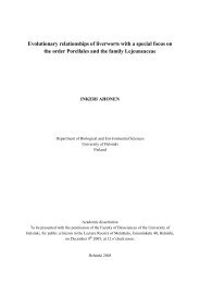
Three diverse sulphidic mines in Finland were 

studied to assess their environmental impacts on 

aquatic biota (Fig.1). The general sampling strategy 

at each site was to provide a sample series 

to detect any possible mine impacts, variations 

in their spatial and temporal extent and distinguish 

them from the effects of other environmental 

variables. Case-specific sampling strategies 

were planned to take into account features such 

as the nature and timing of mining, which were 

slightly different at each site. Three types of corers 

were used: the Limnos gravity corer in PI, PII, 

PIV (Kansanen et al. 1991), a Kullenberg type of 

piston corer in PI (Putkinen & Saarelainen 1998) 

and a Kajak-type gravity corer in PIII (Renberg 

& Hansson 2008). In papers II and III, sediment 

cores were dated with the 1986 Chernobyl 137Cs 

fallout peaks, often detectable in Finland; otherwise, 

we used mine-related geochemical proxies 

for relative dating. Limnological measurements 

and lake physiography data found in the following 

site descriptions are taken from the OIVA database 

of environmental and geographical information, 

30.5.2012. The database is maintained by 

Finland’s environmental administration. 

2.1.1 Luikonlahti (PI, PII) 

The Luikonlahti mine is a Cu-Co-Ni-Zn mine in 

2 MATERIALS AND METHODS 

2.1 Study sites and sampling 

Kaavi, eastern Finland (62°56’N, 28°42’E) on the 

shore of Petkellahti Bay, a part of Lake Retunen 

(Fig. 1). The lake area covers 264,851 ha with an 

average depth of 4.9 m and a maximum depth of 

21.2 m. The catchment of the lake mainly consists 

of sandy till with some smaller areas of finegrained 

material. Chlorophyll–a concentrations 

in Petkellahti bay have fluctuated between 5–20 

µg/l following the peak (45 µg/l) in 1990, but now 

seem to be settled around 5–10 µg/l (2005−2012). 

According to Organization for Economic Co-Operation 

and Development (OECD), the chlorophyll–a 

limit of lakes in a eutrophic state is 8 µg/l. 

The mine was in operation during 1968–1983, 

but mining-related activities predate the actual 

mining period in the area. A total of 7 Mt of ore 

were extracted during the active period. On average, 

the ore contained 0.99% Cu, 0.61% Zn, 0.11% 

Co and 17.22% S (Eskelinen et al. 1983). The processing 

plant was also used to process talc ore 

during 1979–2006. Talc processing produced Ni 

concentrate as a by-product, but the facility has 

been shut down since 2007. Operation of the mill 

is planned to start again after renovation in 2012. 

The Luikonlahti mine is the single most important 

factor affecting the water quality of the Myllyoja 

stream, which is the main water source of the 

bay. Present metal loading is mainly caused by the 

weathering of sulphide-bearing waste rocks and 

12

o 


Luikonlahti 

20 E 

o 

30 E 

16 RET 23b 

Finland 

Lake 

Retunen 

15 

12 

13 

14 

6 

7 

8 

9 

11 10 

5 

4 

3 

2 

RET 99 

Petkellahti 

Bay 

1 

Myllyoja 

Stream 

Waste 

rocks 

Palolampi 

Pond 

66,5 N 

o 

Pyhäsalmi 

Seepage 

Luikonlahti 

Settling 

Pond 

Haveri 

500 m 

60 N 

o 

Outlet 

Pyhäsalmi 

Haveri 

Outflow 

10-6 5-1 

PYHÄJÄRVI 

Junttiselkä 

basin 

Lake 

Kirkkojärvi 

HAV2 

Viljakkalanselkä 

HAV4 

11 - 15 

VILJAKKALA 

500 m 

Kirkkoselkä 

basin 

16 - 25 

Stream 

Road 

Sample site 

Tailings 

N 

2 km 

Railway 

Mine 

Fig. 1. The locations of Luikonlahti, Haveri and Pyhäsalmi mines in Finland, and the detailed sampling maps of the study 

sites. Note the two separate basins in Lake Pyhäjärvi, Junttiselkä and Kirkkoselkä, that were sampled near the Pyhäsalmi mine. 

low pH seepage waters from the tailings area, but 

other human activities, e.g. forest management 

and ditching of the wetlands, have also affected 

water quality in the bay. Furthermore, because of 

the local bedrock, glacial tills in the area contain 

elevated concentrations of S and metals (Koljonen 

1992). However, loading from the mine has 

diminished in recent years. 

Geochemical analyses were performed on 32 

short sediment cores retrieved from the embayment, 

and 16 of these were selected for palaeoecological 

analyses based on water depth at the 

coring site. Each core was subsampled to give a 

modern, mine-impacted ‘top’ sample and a predisturbance 

‘bottom’ sample. This approach was 

used to detect the spatial extent of mine loading 

in the bay and the possible natural gradients existing 

before the mine impacts. Samples were selected 

based on a thin, light mineral layer visible 

in all cores, which was assumed to mark the onset 

13



of mining, or more specifically the drainage of 

the Palolampi pond and other land clearance in 

the area. The depth of the mineral layer varied 

within the bay, and because recent top samples 

were taken above it, up to the surface, top sample 

thicknesses varied with the coring location. 

The second study (PII), however, showed that the 

mineral layer dates the end of the mining period 

instead of the beginning, and the mine-impacted 

samples thus represent the post-mining period. 

The 10- cm-thick ‘bottom’ samples were taken 10 

cm below the marker layer in all cores. In addition 

to this ‘top–bottom’ transect, one low-resolution 

sediment core and two short sediment cores with 

1-cm sample intervals were retrieved and analyzed 

to obtain records of the temporal evolution of the 

mine impacts. One of the short cores was taken 

from a mine-impacted site and the other was considered 

as a reference site outside the Petkellahti 

Bay. 

2.1.2 Haveri (PIII) 

The closed Haveri Cu-Au-mine is located between 

two lake basins in Ylöjärvi, SW Finland (61°43’N, 

23°14’E). The studied basins, Kirkkojärvi and 

Viljakkalanselkä (Fig. 1), are small and separated 

basins of the Kyrösjärvi lake system with a total 

area of 9606.61 ha. The area is generally rural 

with cultivated land and forests and the soils 

mainly consist of fine-grained material (clay, silt). 

This part of the lake system is currently meso-eutrophic 

with an epilimnetic total phosphorus (TP) 

concentration of 20–24 lg/L and a pH of 6.6–7.4, 

measured at the strait between Lake Kyrösjärvi 

and Lake Kirkkojärvi in 1996–2002. Trophic level 

seemed to have elevated from 1992, when total 

phosphorus in Viljakkalanselkä basin was 14 µg. 

The most active period of mining was during 

1942–1962, but small-scale Fe mining occurred 

in the area in the 18th to 19th centuries. Tailings 

have been piled on a cape protruding into the basin 

called Lake Kirkkojärvi. The main sulphide 

minerals in the ore and in the tailings are pyrrhotite, 

chalcopyrite, magnetite and pyrite, of which 

pyrrhotite is the most oxidizable and chalcopyrite 

the most stable. The uppermost layers of the sulphidic 

tailings have oxidized and produce metalrich 

AMD (Parviainen 2009), which affects the 

stream water quality discharging to the lake. 

Two short sediment cores were studied. Kirkkojärvi 

bay has three gentle sloping depressions, 

and the coring site HAV2 was situated in the deepest 

one (7.6 m, diameter ~300 m) in the middle 

of the bay. It was located near the tailings pile to 

represent a ‘mine-impacted site’, while the deeper 

HAV4 site in the Viljakkalanselkä basin was located 

in the wide mid-basin with a depth of 22 m, 

further ‘upstream’ from the mine, as a reference 

site. The reference site was also used to evaluate 

nutrient enrichment in the area and to distinguish 

its effects from the mine impacts. Both cores were 

sectioned into continuous slices, HAV2 into 1-cm 

slices, while HAV4 was sectioned into 1-cm slices 

down to 10 cm and into 2-cm slices further down. 

This sampling strategy made it possible to follow 

the temporal changes in the geochemical nature 

of the mine loading and the corresponding ecological 

shifts. 

2.1.3 Pyhäsalmi mine (PIV) 

The Pyhäsalmi Zn-Cu-S mine is located in the 

town of Pyhäjärvi, central Finland, on the shore 

of the relatively large (12178.5 ha) and shallow 

(mean depth 6.27 m, max depth 27 m) Lake Pyhäjärvi 

(63° 24 N, 25° 58 E). Two of Lake Pyhäjärvi’s 

lowest basins, Junttiselkä and Kirkkoselkä, 

were included in the study. The catchment 

of both basins mainly consists of ditched peatland 

and cultivated fine grained till. The lowest, smaller 

and quite closed Junttiselkä basin has higher 

nutrient and humus concentrations and it has 

suffered from oxygen depletion and internal loading 

of metals and nutrients. During 2000–2012, 

epilimnetic total phosphorus (TP) concentrations 

in Junttiselkä have fluctuated (12–50 µg/l), but the 

average is 25 µg/l. In Kirkkoselkä basin, the TP 

average is 13 µg/l (6–23 µg/l). The same difference 

in the trophic level of the basins is seen in chlorophyll-a 

concentrations: Junttiselkä 6–24 µg/l (~12 

µg/l) and Kirkkoselkä 2–9 µg/l (~5 µg/l). The pH 

in both basins has been quite stable and neutral, 

~6–7, being slightly lower in Junttiselkä. 

The mine has been in operation from 1962 and 

is still under production. Metal-rich mine loading 

to the lake was at its highest in the 1970s and 

1980s, and the main outlet for mine waters was 

located by the Kirkkoselkä basin next to the tailings. 

Currently, liming is used to precipitate the 

metals in the tailings area, which has reduced the 

metal concentrations of recent effluents. Modern 

mine loading thus mainly consists of Ca and S, 

which makes the wastewaters dense and nearly 

saturated with gypsum (CaSO 4 

). The loading site 

has also changed from Kirkkoselkä to the Junttiselkä 

basin. 

Sampling was aimed to cover both the temporal 

and spatial extent of the mine loading in the 

basins. Short sediment cores were retrieved from 

25 sample sites in a transect: 10 ‘downstream’ and 

15 ‘upstream’ from the mine (Fig. 1). The sam- 

14


pling interval was 2 cm on each core. Exploratory 

XRF analysis of Cu and Zn was used to select 

three sample levels from each core to represent 

phases immediately before the mine, during peak 

metal loading and the present situation. These 

three subsampling levels form stratigraphically 

correlated temporal horizons of each time period 

to provide a spatial profile of the mine impacts for 

each loading phase. 

2.2 Geochemical analyses 

A microwave-assisted HNO 3 

digestion method 

(3051; US EPA 1994) was used for geochemical 

analyses on freeze-dried samples in all cases. In 

addition, the mine-impacted ‘top’ samples of the 

Luikonlahti case (PI) were analyzed using 1M 

ammonium acetate leach. All analyses were performed 

in accredited testing laboratories of the 

Geological Survey of Finland (PI, PII) and Labtium 

Ltd (PIII, PIV). HNO 3 

extraction breaks 

down sulphides, most salts (e.g., apatite), carbonates, 

trioctahedral micas, 2:1 and 1:1 clay minerals 

and most of the talc, and provides a record 

of mine-derived elements. It does not, however, 

dissolve major silicates such as quartz, feldspars, 

amphiboles or pyroxenes. The method can extract 

certain fractions that are not bioavailable and the 

sediment concentrations should not be interpreted 

to have been biologically available at the time of 

deposition. However, the stability of the concentrations 

makes them more suitable to use as proxies 

of the mine water loading than those obtained 

with weaker extractions such as ammonium acetate 

leach. The 1M ammonium acetate solution 

used at Luikonlahti (PI) extracts chemically adsorbed 

elements from solid surfaces. Depending 

on the sample type, this 2-h extraction liberates 

elements with cation exchange capacity and those 

complexed on solid surfaces, and dissolves carbonates 

(excluding magnesite) and hydroxide precipitates 

such as poorly crystalline ferrihydrite. It 

was considered to be a more biologically relevant 

fraction, and was thus chosen to represent possible 

bioaccessible fraction of elements. 

For specific element determinations in all case 

studies, both ICP-MS and ICP-AES were used, 

depending on the element. Leco and CN analyzers 

were used to determine sulphur, carbon and 

nitrogen concentrations. In addition, in the Pyhäsalmi 

case (PIV), exploratory XRF analysis of 

Cu and Zn was performed with an X-met® 3000 

TXS+ analyzer (Oxford Instruments). 

Organic and water contents were measured by 

loss on ignition. Samples were first weighed, then 

dried overnight at 105 °C and finally ignited for 

two hours at 550 °C. 

2.3 Thecamoebian analyses 

2.3.1 Sample procedures 

Thecamoebian analyses were carried out with 

~1–3 g samples of fresh weight sediment. The water 

content of the samples was taken into account 

when weighting them. The samples were sieved 

with distilled water through 500 and 56 µm meshes 

in order to remove coarse organics and silt and 

clay-sized particles, but to retain testate amoebae. 

Sieved samples were divided into 8 aliquots using 

a wet splitter described by Scott and Hermelin 

(1993) to optimize the number of tests for counting 

while retaining statistical significance. Most 

of the time a few samples were enough, but the 

reference core of Haveri case (PIII), in particular, 

required systemically more samples, despite the 

sample sizes being in the upper part of the scale 

(~3 g). Mechanical stress was avoided so as not 

to break the tests. The smaller mesh size we used 

falls in the range often used in thecamoebian research 

(30–63 µm), but smaller thecamoebians do 

exist (down to 10 μm; Beyens & Meisterfeld 2001). 

These were lost during sieving, causing systematic 

bias in the results in each case. At least ~200–250 

specimens per sample were counted immersed in 

water. In a few samples thecamoebians were not 

abundant enough, resulting in a lower final count. 

Specimens were identified and counted using stereomicroscopes: 

Nikon SMZ-1B 8×−35× (PI), 

Wild M3Z (6.4–809) (PII) and Olympus SZH 

(7.5–64) (PII, PIII, PIV). Some specimens from 

Pyhäjärvi (PIV) were also photographed using a 

JEOL JSM 5900LV scanning electron microscope. 

2.3.2 Identification and the species problem 

Identification of thecamoebians was mainly 

based on the wide cluster mode of classification 

of Medioli and Scott (1983) (PI, PII, PIII, PIV), 

and the identification key of Kumar and Dalby 

(1998) (PII, PIII, PIV), but additional references 

were used as well (e.g. Asioli et al. 1996 PI, 

15



PII, Reinhardt et al. 1998, Charman et al. 2000, 

Ogden & Hedley 1980, Leidy 1879). None of the 

papers were taxonomic in nature, and there was 

some taxonomic variability in identifications. To 

clarify this confusion, a taxonomic listing that 

also describes how the naming and definition of 

certain forms has evolved from paper to paper is 

provided (Appendix 1) together with sheets of the 

raw data (Appendix 2). Raw environmental data 

is available on request from the author. Most of 

the variability was associated with the definition 

of strains of Difflugia protaeiformis. Some strains 

of Difflugia species were left unidentified in the 

Luikonlahti case (PI), but were later identified as 

strains of D. oblonga (PII). Strains of C. constricta 

were not differentiated at Luikonlahti (PI, PII), 

and in the Pyhäsalmi case (PIV) Centropyxis constricta 

‘spinosa’ and ‘constricta’ were combined. 

2.4 Diatom analysis 

In the Haveri case (PII), diatom analyses were 

carried out alongside thecamoebian analysis to 

examine the similarities and differences between 

these two proxies. Both proxies were subjected 

to same unconstrained and constrained (PCA, 

RDA, see below) multivariate methods. Krammer 

and Lange-Bertalot (1986, 1988, 1991a, b) were 

mainly used as a reference for identification. The 

responses of diatom assemblages to nutrients and 

pH were studied using inference models developed 

for total phosphorus (TP) concentrations and pH. 

TP was reconstructed with the inference model of 

Kauppila et al. (2002). A detailed description of 

sample procedures and the inference models used 

can be found in paper III. 

2.5 Numerical methods 

2.5.1 Ordinations 

Thecamoebian results of each case study were 

summarized using indirect and direct multivariate 

statistical methods. All analyses and visualizations 

were carried out using the CANOCO 4.5 WIN 

and CanoDraw software package of ter Braak 

and Šmilauer (2002). Species data were first subjected 

to exploratory detrended correspondence 

analysis (DCA) to determine the length of the 

faunal gradient. On the grounds of this (100% increases over their respective 

threshold effect concentrations (TECs) for 

freshwater sediments. The TECs were based on 

NOAA Screening Quick Reference Tables (Buchman 

2008). The resulting variable (sum metal toxicity) 

was included as an environmental variable 

in the RDA model alongside other geochemical 

variables that were selected to represent sediment 

quality (C), clastic input (Ti), present loading 

(Ca), redox conditions (Mn) and eutrophication 

16


(C/N). RDA was constrained for each temporal 

horizon, but also separately for both basins with 

all three temporal horizons included. 

2.5.2 Other indices 

Thecamoebian data sets were also defined by species 

diversity indices, which were calculated using 

the PAST program version 1.68 (Hammer et al. 

2001). Stressed environmental situations may reduce 

the diversity of the species composition and 

lead to the domination of only a few resistant and 

opportunistic taxa (Patterson & Kumar 2000a). 

The Shannon index (H), which ranges from 0 for 

samples with only a single taxon to higher values 

for samples with many taxa, each represented by 

few individuals, were used in all papers. A healthy 

thecamoebian fauna has Shannon diversity index 

> 2.5 (Patterson & Kumar 2000a). The Berger- 

Parker dominance index, which gives the proportion 

of the dominant taxon in the sample, was 

used in papers II, III and IV. Distance measures 

were used to study amount of change in faunal 

compositions. The amount of faunal change between 

top–bottom sample pairs (PII) and the 

pre-, peak- and post-sample horizons (PIV) were 

determined as Euclidean and chord distances calculated 

by the PAST program version 1.68 (Hammer 

et al. 2001). The same distance measures were 

also used in exploratory clustering with the paired 

group method in papers II and III. 

3 RESULTS AND DISCUSSION 

3.1 Geochemical gradients in the case studies 

Temporal changes in the magnitude and composition 

of mine water loading were observed in 

all cases. The temporal geochemical results had 

similar general features, regardless of the study 

site in question. At Haveri and Pyhäsalmi (PIII 

and PIV), the first mine-related changes showed 

as an increased clastic input into the lakes, with 

higher concentrations of elements such as Ti, K, 

Na and Mg. This phase preceded the metallic 

contamination (PIII) and may be directly related 

to the beginning of mining and construction of 

the mine, but could also result from some other 

change in the regional land use. The mine-impacted 

sediment core HAV2 from Lake Kirkkojärvi at 

Haveri (PII) showed clearly increasing concentrations 

of clastic input-related elements before the 

metal contamination peaks. This feature was not 

detectable at the reference site HAV4. Instead, 

loss on ignition increased profoundly at this stage, 

probably because of ongoing changes in regional 

land use and eutrophication. At Pyhäsalmi (PIV), 

the land use-related changes were observed in a 

different manner because of the diverging sampling 

strategy. No sediment cores were analyzed 

throughout, but samples of the peak loading horizon 

already had clearly elevated concentrations 

of clastic input-related elements. In contrast, 

similar increases in mineral matter inputs were 

not recorded in the impacted RET99 core next to 

the Luikonlahti mine (PII). Instead, the onset of 

mining coincided with a decrease in Ti levels and 

fluctuation in Mg and Cr levels, if anything. However, 

S concentrations increased sharply before 

the highest metal loading (Fig. 2). Furthermore, 

the water content of the sediment increased, linking 

these changes to an increase in the organic 

matter inputs. In these samples, concentrations of 

mine-related metals also seem to have slightly increased, 

a feature additionally found in the Haveri 

sediment cores before the peak loading phase. 

A phase of peak metal contamination followed 

these first geochemical changes at each mine site. 

In the impacted Haveri core (PIII) it showed as 

two consecutive metal peaks, with Cu and Ni 

peaking first and other metals such as Ag, As, 

and Zn following a few years later. S, Pb, Co and 

Cd also increased, but not as sharply as the other 

metals. The same feature was shown in the reference 

core, but the two peaks were merged because 

of the thicker subsamples (lower temporal resolution). 

In the mine-impacted core from Luikonlahti 

(PII), geochemical features of the peak 

metal loading were notably different. Co and Cu 

peaked sharply at the beginning of the 1980s and 

have since decreased, but not to their background 

levels. In contrast, Ni and Zn reached their peak 

concentrations in the top 10 cm of the core. In 

the Luikonlahti reference core, concentrations of 

metals and S were highest in the 10 topmost centimetres 

(PII). 

Spatial trends were studied in more detail in the 

Luikonlahti (PI, PII) and Pyhäsalmi cases (PIV). 

At Pyhäsalmi, the spatial extent of the highest 

metal peaks remained limited to a few sites in the 

Kirkkoselkä basin, close to the tailings area, even 

though concentrations in the peak loading phase 

17



4000 

Haveri Luikonlahti Pyhäsalmi 

Post Peak Pre 

Cu 


Post Peak Pre 

S 

22000 

3000 

16500 

2000 

11000 

1000 

5500 

0 

0 11 20 25 4 10 22 10-1 11-25 10-1 11-25 10-1 11-25 0 11 20 25 4 10 22 10-1 11-25 10-1 11-25 10-1 11-25 

Sample depth(cm) Sample site Sample depth(cm) Sample site 



Post Peak Pre 

Post Peak Pre 

3500 

3000 

Ti 

Zn 

0 

3500 

3000 

2500 

2500 

mg/kg 

2000 

1500 

2000 

1500 

mg/kg 

1000 

1000 

500 

500 

16000 

14000 

0 

0 11 20 25 4 10 22 10-1 11-25 10-1 11-25 10-1 11-25 0 11 20 25 4 10 22 10-1 11-25 10-1 11-25 10-1 11-25 

Sample depth(cm) Sample site Sample depth(cm) Sample site 


Post Peak Pre 

Ca 


Post Peak Pre 

Ni 

400 

350 

12000 

300 

10000 

250 

8000 

200 

6000 

150 

4000 

100 

2000 

50 

0 

0 11 2025 4 10 22 10-1 11-25 10-1 11-25 10-1 11-25 

Sample depth(cm) 

Sample site 

0 11 2025 4 10 22 10-1 11-25 10-1 11-25 10-1 11-25 

Sample depth(cm) 

Sample site 

Pre disturbance Active mining Peak loading Post disturbance 

Fig. 2. Geochemical results for various elements (Cu, S, Ti, Zn, Ca and Ni) in the profiles of mine-impacted sediment cores 

from Haveri and Luikonlahti and Pyhäsalmi sediment sample transects, all placed horizontally. Samples in the sediment profiles 

of Luikonlahti and Haveri are divided into four groups: pre-disturbance (green), active mining (orange), peak loading 

(red) and post-disturbance (yellow). Pyhäsalmi samples are in three transect-forming groups: pre-disturbance (green), peak 

loading (red) and post-disturbance (yellow). 

18


samples were in general higher than in the pre-disturbance 

samples in both basins under study. At 

Luikonlahti, the modern top sediment samples illustrated 

a more complex picture of the elemental 

distribution in the investigated bay area. The spatial 

pattern of contamination and the geochemical 

gradients varied with distance from the source 

(dispersion and dilution), water depth (redox and 

pH) and time (from clastic inputs towards colloids 

and low pH). In the Luikonlahti case, too, 

it seemed that the strongest metal contamination 

was confined to the four closest sites from the 

stream mouth, the source of mine loading. 

Despite the similarities, the geochemical fingerprint 

in the mine-impacted samples (and thus 

the nature of environmental forcing on biota) 

was substantially different in each case. Figure 2 

points out some of these differences between the 

case studies. First of all, Ti, an element that has 

been widely used to represent the mineral matter 

supply, illustrates the clear difference between 

the Haveri cores and sediments in the other lakes. 

This element also clearly illustrates the succession 

in the Pyhäsalmi case, towards increased clastic 

sedimentation, but also shows the difference between 

the two lake basins. Ti concentrations in 

Luikonlahti sediments were lower but strongly 

fluctuating, following the concentrations of other 

mineral matter-related elements (i.e. K, Na, Mg). 

There were also major differences in the peak 

concentrations of sulphur and metals between the 

mine sites. Peak concentrations of S were several 

times higher at Luikonlahti than in the other cases. 

Only some of the peak loading samples from 

Pyhäsalmi had such high levels of S. In addition, 

there was considerable variation in the peak concentrations 

of metals. Zn concentrations were 

highest in the Pyhäsalmi peak samples, Cu concentrations 

at Haveri, and the highest Ni concentrations 

were found at Luikonlahti. At Haveri, the 

Ni concentrations were somewhat elevated, but at 

Pyhäsalmi they were constantly low. Some other 

metals that are not shown in Figure 2 were also 

distributed unevenly: Pb and Cd peaked in the 

samples from the Kirkkoselkä basin at Pyhäsalmi 

and remained elevated after the changes in mine 

water loading. Co peaked in the Luikonlahti peak 

contamination samples, while at Pyhäsalmi the 

elevated Co concentrations were related to redox 

conditions in the Kirkkoselkä basin rather than to 

mine-derived contamination. 

A PCA on the geochemical variables summarizes 

the clear division between the sites and 

samples (Fig. 3). The Haveri samples showed only 

-0.4 1.0 

K 

Cr 

Na 

Mg 

Ti 

Ca 

S 

Al 

Cu 

Pb 

Cd 

Zn 

Ni 

-0.6 1.2 

P 

Mn 

Co 

As 

Haveri 

Luikonlahti 

Junttiselkä 

Kirkkoselkä 

Pre disturbance 

Mining actitivity 

Peak loading 

Post disturbance 

Fig. 3. A PCA diagram of the geochemical distribution of Pyhäsalmi sediment from Junttiselkä and Kirkkoselkä lake basins 

and the mine-impacted sediment cores of Haveri and Luikonlahti. Haveri and Luikonlahti samples are divided into four 

groups: pre-disturbance (green), active mining (orange), peak loading (red) and post-disturbance (yellow). Pyhäsalmi transects 

have three sample horizons: pre, peak and post. 

Fe 

19



little variation, whereas the Kirkkoselkä samples 

of the Pyhäsalmi case showed a clear succession 

along the second axis from the pre-disturbance 

conditions to the present, post-disturbance situation. 

The Junttiselkä samples remained in the 

left half of plot with the temporal horizons mixed 

together. Only the pre-disturbance samples separated 

slightly. The Luikonlahti samples are spread 

along the first axis, but almost every sample plotted 

in the lower half of the diagram with Co, Ni 

and S. 

3.2 Distribution of thecamoebians 

Basic features of the faunal assemblages were 

quite similar in all of the lakes studied, and an abbreviated 

taxonomy with the authors or descriptions 

of found forms is provided in Appendix 1. 

A large part of the assemblages consisted of different 

forms of Difflugia oblonga, especially in 

the undisturbed samples and in less environmentally 

stressed environments such as in the Kirkkoselkä 

basin in the case of Pyhäsalmi (PIV). In 

the sediment cores from Luikonlahti (PII) and 

Haveri (PIII) their proportion decreased towards 

the surface, mostly because of the increase in the 

proportion of Cucurbitella tricuspis. Despite this, 

forms of D. oblonga were always abundant. The 

species has been connected gyttja and it has been 

found to be ubiquitous when the substrate is sufficiently 

organic (McCarthy et al. 1995). The diverse 

group of strains of D. oblonga could possess 

an even more specific indicator potential, but the 

strains are often challenging to distinguish from 

each other and leave the identifications open to 

subjective interpretation. In the present studies, at 

least one of the strains of D. oblonga showed clear 

signs of indicator value (PIV): The strain ‘spinosa’, 

a form that has been reported in previous 

studies by Patterson et al. (1985, 2002) and Boudreau 

et al. (2005), was spatially and temporally 

distinctly distributed in the Pyhäsalmi case. It was 

clearly connected to the increased clastic input as 

well as to an increase in Ca concentrations, thus 

being related to a clayey substrate, high conductivity 

and/or alkalinity. Previous studies from the 

Greater Toronto Area, Canada (Roe et al. 2010), 

subtropical Florida (Escobar et al. 2008) and Ontario, 

Canada (Reinhardt et al. 1998) support this 

suggestion. In contrast, increasing abundances of 

C. tricuspis suggested a general increase in the nutrient 

level and trophic status of each of the study 

lakes. C. tricuspis is a species known to indicate 

eutrophication (Scott & Medioli 1983, Patterson 

et al. 1985, Asioli et al. 1996, Boudreau et al. 2005, 

Reinhardt et al. 2005, Roe et al. 2010). This succession 

was shown most clearly in the sediment 

cores of the Luikonlahti and Haveri cases (PII, 

PIII), but also in the Pyhäsalmi case (PIV), especially 

in the presently eutrophic Junttiselkä basin. 

Another important cluster of thecamoebians 

included strains of Difflugia protaeiformis. In 

these studies, the most promising environmental 

indicator form was the strain ‘multicornis’ (referred 

as D. protaeiformis ‘strain A’ in PI, and 

Difflugia fragosa in PII) . At Luikonlahti (PII), 

it was linked to increased levels of Ca, Ni and 

Zn and decreased concentrations of the clastic 

input-related elements K, Na, and Mg. Such conditions 

developed after the mine switched to talc 

processing (PII). At Haveri (PIII), the strain was 

connected to the beginning of the mining activities 

and increasing clastic input, including Ca. At 

Pyhäsalmi the form increased in abundance in the 

peak loading samples and was statistically significantly 

related to Ca, and thus to water hardness 

and pH. Other forms of D. protaeiformis were also 

abundant in the present cases. Asioli et al. (1996) 

connected D. proteiformis [sic] ‘proteiformis’ with 

an environment rich in organics and sulphides 

and low in oxygen, while the form ‘rapa’ was connected 

to strongly polluted environments. These 

forms, however, do not fully match with our classification 

(see taxonomic listing Appendix 1). Despite 

the slight variation in the taxonomy, the occurrence 

of strains ‘acuminata’ and ‘claviformis’ 

are probably linked to sediment quality in terms 

of organic content (PIV) and the strain ‘amphoralis’ 

may have some indicator value for metal 

contamination. The latter correlated with the 

metal sum toxicity at Pyhäsalmi (PIV), was part 

of the mine-impacted species assemblage in Lake 

Retunen (PII) and occurred in the metal- (Co and 

Pb) and nutrient-rich group at Haveri (PIII) 

Different forms of centropyxids made up a considerable 

part of all of the species assemblages. 

Forms of Centropyxis aculeata were more abundant 

than Centropyxis constricta, but the latter 

seems to have more specific indicator value. Centropyxids 

are a group of thecamoebians that have 

been considered to be opportunistic and tolerant 

of extreme conditions. They have been found to 

withstand various stressed environmental conditions 

such as metal-rich waters (Patterson et al. 

1996, Reinhardt et al. 1998), high concentrations 

of naphthenic acids from oil sand mining (Nev- 

20


ille et al. 2011), slightly brackish environments 

(Scott & Medioli 1983, Patterson et al. 1985), 

lakes contaminated by road salt (Roe et al. 2010), 

oligotrophic, turbid and low production environments 

(Burbidge & Schröder-Adams 1998), and 

low oxygen concentrations (Reinhardt et al. 1998, 

Roe et al. 2010). In all the cases in this study (PII, 

PIII, PIV), C. constricta ‘aerophila’ seemed to be 

connected with high metal and S concentrations, 

although it still occurred in low numbers. Some 

variability in identification complicates the discussion 

regarding C. aculeata, but the form seemed 

to be connected with metal maxima in the peak 

loading samples in the Pyhäsalmi case (PIV). C. 

constricta ‘aerophila’ and C. aculeata ‘discoides’ 

were also found to be the most opportunistic in 

a seasonal study on an oil sands reclamation wetland 

in northern Alberta (Neville et al. 2010a). 

However, the quality of the substrate and perhaps 

also water turbulence affected the species, since it 

appeared in greater numbers near the outlet on 

the Junttiselkä basin and close to the Tikkalansalmi 

strait. The suggested connection of C. aculeata 

with metals and mining operations could also be 

found in the results from Luikonlahti and Haveri. 

In addition to the common, ubiquitous species 

and strains, the thecamoebian assemblages 

included species with minor proportions at all 

mine sites. These less abundant species included 

Pontigulasia compressa, Lesquereusia spiralis, 

Difflugia urceolata, Lagenodifflugia vas, Difflugia 

bidens and Arcella vulgaris. Some of these forms 

showed potential indicator value, while others appeared 

to be mostly indifferent to environmental 

gradients occurring in these studies. Of the environmentally 

sensitive species, D. bidens has previously 

been connected to high terrigenous inputs 

(Patterson et al. 1985) and clear cutting of forest 

(Scott & Medioli 1983). The same was noticeable 

in the Pyhäsalmi case (PIV), where D. bidens was 

almost absent from the pre-disturbance samples, 

but appeared in peak loading samples and increased 

in numbers in recent sediments, together 

with mineral matter. In contrast, L. spiralis was 

present in every case, being only slightly less abundant 

in ‘background’ sediment cores from deep 

water in the cases of Haveri and Luikonlahti (PII, 

PIII). Patterson and Kumar (2000b) connected 

this species with coarser, sandier substrate, and 

the same connection was suggested in all the cases 

of the present study. The species was found in 

higher proportions in the basin with a higher clastic 

sedimentation rate at Pyhäsalmi (PIV) and increased 

in numbers when the mining activities and 

changes in the land-use began and the transport 

of coarser matter into the lake increased (PII, 

PIII, PIV). This is supported by the observations 

of lower numbers of L. spiralis in the deeper water 

samples, where the sediment grain size is usually 

finer. Besides these indicator species for substrate 

quality, L. vas appeared to be affected by pH and 

Ca in the Luikonlahti sediment core (PII), but this 

remains inconclusive. 

In addition to the distribution of individual 

species and strains, the species diversities of the 

faunal assemblages showed similar patterns from 

case to case. Especially the increase in the abundance 

of C. tricuspis caused lower diversity at 

Luikonlahti and Haveri (PII, PIII). On the other 

hand, in the reference core of Haveri, diversity 

increased in the peak loading samples instead 

of the opposite. The reference core had initially 

lower species diversity, and when opportunistic 

thecamoebian forms appeared in the assemblage 

with metal contamination, diversity increased. 

The core was retrieved from deeper water, which 

may be the reason for the generally lower diversity. 

This relationship between water depth and 

diversity has been found in lacustrine diatoms 

within a basin (Kingsbury et al. 2012). 

3.3 Relationships between thecamoebians and environmental variables 

Numerical analyses were employed to study the 

aquatic mine impacts and to distinguish between 

the effects of different environmental factors. 

RDA and linear correlations between thecamoebian 

PCA axis sample scores (i.e. the variation 

in faunal assemblages) and the corresponding 

geochemical concentrations were used to find 

the relationships between faunal features and 

environmental variables. The observed relationships 

between testate amoebae and geochemical 

variables are summarized in Table 1. Generally, at 

Luikonlahti, the most important environmental 

factors seemed to be related to the overall geochemical 

conditions, such as pH and redox conditions, 

whereas the Haveri results showed the 

clearest connection between metals and amoebae. 

At Pyhäsalmi, the strongest relationships between 

faunal assemblages and environmental variables 

were linked with the present Ca and SO 4 

-rich 

loading, redox conditions, trophic status of the 

lake and substrate composition. 

The results from Luikonlahti pointed to effects 

of factors such as redox conditions, substrate 

quality, Al, Cr, Cu, and Zn on thecamoe- 

21



Table 1. Summarized relationships between environmental variables and thecamoebians of all the case studies; marginal effects 

(RDA), conditional effects (RDA) and correlations (with PCA axis scores). 

Marginal Effects (RDA) 

Luikonlahti: 

Surface transect: Al, Cr, Mn, Fe and Ba * 

Fe:Mn, S, C, P, 

Conditional 

effects (RDA) 

Fe:Mn, Al and Mn 

EFs: Al, Cr, and Zn 

Correlations with PCA axis scores 

Not analyzed 

Impacted core 

(Ret99): 

Not analyzed Not analyzed Axis 1: Ca, Zn, Fe, Fe:Mn, Co, Cu, and Ni 

Axis 2: Al 

Other: 

Top-Bottom pairs (EFs): Cu, -Pb, C, N Al, Cr, Zn 

Haveri: 

Impacted core: Co, Pb, P, LOI, Cd, U Not analyzed Axis 1: Co, P, LOI, Al, B, Fe, Mn, Pb 

Axis 3: -S, -Mo, -Ni, -Cu 

Reference core: Ag, Cu, As, Mo, and Zn Not analyzed Axis 1: Mg, K, Ti, –LOI, –Ba, –P, – 

Cd, –Sr, –Sb, –Mn, –Co, –Pb 

Axis 2: Zn, Ag, Cu, Mo, Ni, Bi, S, As. 

Pyhäsalmi: 

Pre disturbance: 

Peak loading: 

Post disturbance: 

Junttiselkä: 

Mn, Ca and C:N 

Ca, Ti 

C:N, Ti, Ca Mn 

C, Ti, Ca, Mn, C/N, 

metal sum tox 

Mn 

Kirkkoselkä: Ti, C:N, Ca C:N, Metal 

sum tox, C 

* NH4Ac-leached 

Not analyzed 

- Not analyzed 

Not analyzed 

bians. RDA marginal effects for the Luikonlahti 

surface sediment sample transect showed statistically 

significant relationships between faunal 

changes and six environmental variables. 

NH 4 

Ac-leached Cr, Al, and S, as well as the 

Fe:Mn ratio, decreased away from the source 

of pollution, while the concentrations of Ba 

and Mn increased. Conditional RDA analysis 

reduced the number of statistically significant 

variables to three: Fe:Mn, Al and Mn. In the 

second study from Luikonlahti (PII), concentrations 

of S, C, P, and the NH 4 

Ac-leached Al, 

Fe, and Mn also showed a significant correlation 

with faunal distribution in the modern sediment 

transect. However, none of the easily leachable 

(‘bioaccessible’, potentially able to interact with 

and be absorbed by organisms) concentrations 

of the major mining related heavy metals (Cu, 

Ni, Zn, Co) had statistically significant relationships 

with the species assemblages. Besides these 

bioaccessible geochemical concentrations in the 

top sediments, bottom-to-top enrichment factors 

(based on HNO 3 

extractions) of Al, Cr, and 

Zn were correlated significantly with the surface 

sediment faunal assemblages. In the top–bottom 

sample pairs, the bottom-to-top faunal changes 

and the corresponding top–bottom enrichment 

factors of Cu, C, N, Al, Cr, Zn and Pb correlated 

significantly. Furthermore, despite the attempt 

to standardize the water depth at coring sites, 

the remaining variation may have affected the 

transect results. In the impacted RET99 core, the 

variables with constantly increasing values from 

the start of the mining period (Ca, Zn) showed 

the highest correlations with PCA axis 1 scores. 

Fe and the Fe:Mn ratio were also highly correlated 

with axis 1 scores for the core samples, suggesting 

the importance of redox conditions. The 

mining-related metals Co, Cu, and Ni correlated 

with axis 1 scores, but the pH-related metal Al 

was the only variable having a statistically significant 

correlation with PCA axis 2. 

In the mine-impacted core from Haveri, the 

highest and statistically significant correlations 

were found between faunal assemblages (PCA 

axis 1) and the variables that remained elevated 

after the post mining metal concentration peak at 

15 cm (Co, P, LOI, Al, B, Fe, Mn, and Pb). None 

of the variables correlated significantly with PCA 

axis 2, but S, Mo, Ni, and Cu, the elements of the 

first geochemical peaking phase, had significant 

negative correlations with Axis 3 sample scores. 

RDA analysis limited the significant correlations 

to Co, Pb, P, LOI, Cd and U. These were again 

22


elements with elevated concentrations in the upper 

part of the core, where the eutrophic C. tricuspis 

dominates the species assemblages. Nutrient 

enrichment may thus have affected the result of 

the analysis without any link to mining effluents. 

In the reference core of Haveri, over half of the 

analyzed elements were statistically significantly 

correlated with faunal PCA axis scores, but the 

variables could be divided into three groups. The 

first group, comprising the mineral matter-related 

elements Mg, K, and Ti, had a positive correlation 

with PCA axis 1, whereas the second group 

with loss on ignition, several heavy metals, and 

P correlated negatively. Organic content had the 

strongest relationship with faunal changes, and all 

these environmental variables increased towards 

the surface of the core. The third group consisted 

of sharply peaking elements at 10–12 cm, i.e. 

Zn, Ag, Cu, Mo, Ni, Bi, S and As, and correlated 

positively with the second faunal axis. The only 

elements that had significant marginal effects on 

faunal assemblages in RDA were Ag, Cu, As, 

Mo, and Zn. These results suggest that eutrophication 

and changes in land use are the dominant 

environmental factors affecting thecamoebian assemblages, 

and mine-induced changes remained 

minor further afield. Thecamoebian and diatom 

responses to the mine-induced changes were 

largely similar, with some differences in relation 

to metals and to the phase after the highest metal 

loading. Both records showed dependence on the 

nutrient enrichment in the water bodies and on 

the composition of mine water inputs. Elements 

with statistically significant marginal effects on 

both proxies were partly the same, but the thecamoebian 

response seemed to be more limited. 

Co, Pb, Cd and U had significant marginal effects 

on both proxies, but diatoms responded to other 

elements as well. Diatom records also showed that 

shifts in algal assemblages during the peak metal 

loading were not caused by the effects of pH or 

nutrients (phosphorus). 

At Pyhäsalmi, the relationships between testate 

amoebae and environmental variables were studied 

with RDA. In the full pre-disturbance dataset, 

with both lake basins included, Mn, Ca and 

C:N attained statistical significance. In the peak 

impact sample transect, only Ca and Ti showed 

statistical significance. Metal sum toxicity was not 

statistically significantly related to thecamoebian 

assemblages, despite the clear trend in geochemistry. 

In the post-disturbance horizon, statistically 

significant variables included C:N, Ti, Ca, 

and Mn. Conditional testing radically limited the 

number of significant variables: only Mn in the 

pre-disturbance samples remained significant. In 

the basin- specific analysis of the Junttiselkä basin, 

all variables except sediment quality showed 

statistically significant marginal effects on species 

data, but none of the conditional effects were significant. 

At Kirkkoselkä, Ti, C:N and Ca had statistically 

significant marginal effects, but only C:N 

had an independent signal in the faunal data. In 

addition, metal sum toxicity and sediment quality 

had significant conditional effects on thecamoebians 

in this basin located by the mine tailings area. 

For the complete dataset, metal sum toxicity did 

not have a statistically significant effect on biota, 

but other environmental variables, substrate quality, 

redox conditions and eutrophication were 

more important factors. 

PCA based on faunal assemblages was also 

used to summarize the pooled results of all case 

studies (Fig. 4). There was relatively high, natural 

variation between the case studies, even with harmonized 

taxonomy. However, the species assemblages 

showed similar faunal successions in relation 

to human disturbance in all case studies (Fig. 

4a). Natural, pre-disturbance samples (shown 

in green) plot on the left on the first axis, but 

are spread along the second axis (Fig. 4b). Predisturbance 

samples from the Kirkkoselkä basin 

(Pyhäsalmi) plot on the upper left, while the Haveri 

and Luikonlahti samples plot down in the left 

quadrant. The Junttiselkä samples lie somewhere 

in between. The combined PCA also suggests 

that the beginning of the mining activities may 

not cause a clear faunal response, since samples 

representing these periods at Luikonlahti and Haveri 

plot with the pre-disturbance samples (Fig. 

4c). Metallic peak loading samples, instead, are 

found in the middle of the diagram with the minerelated 

environmental variables (Fig. 4d). Postdisturbance 

samples from Haveri, Luikonlahti 

and most of the Junttiselkä samples (Pyhäsalmi) 

plot with varying metal concentrations on the 

right half of the diagram, along the first axis (Fig. 

4e). In contrast, post-disturbance samples of the 

rather nutrient-poor Kirkkoselkä basin plot in the 

lower left quadrant of the diagram. These results 

suggest that most of the observed succession is 

due to the increase in a well-known eutrophic indicator, 

C. tricuspis, especially in the Haveri and 

Luikonlahti cases and in the Junttiselkä basin of 

Pyhäsalmi. Post-disturbance samples of the still 

fairly oligotrophic Kirkkojärvi basin, in contrast, 

grouped together with the pre-disturbance samples 

from Haveri and Luikonlahti, suggesting that 

they have been largely unaffected by the nutrient 

increase. These results thus clearly show that human-induced 

eutrophication often overshadows 

the mine-related changes in faunal assemblages. 

23



-1.0 1.0 

-0.8 0.8 

a) 

DIFoblLI 

DIFoblBR 

Fe 

As 

Mn 

P 

Co 

DifPROam 

DIFoblTE 

PONcom Lvas 

DIFoblOB 

Pb CuS 

Zn 

Cd 

Ni 

Ca 

Al Na 

K 

CrTi 

Mg 

-0.8 0.8 

DiPROac 

CENcons 

CENacu 

CENconAE 

DifPROcl 

Lespi 

DifPROmu 

CUCtri 

Haveri 

Luikonlahti 

Junttiselkä 

Kirkkoselkä 

Pre disturbance 

Mining actitivity 

Peak loading 


-1.0 1.0 

Fig. 4 a, b, c, d, e. PCA diagrams of harmonized thecamoebian assemblages of Pyhäsalmi (Junttiselkä and Kirkkoselkä basins) 

and the mine-impacted sediment core samples of Haveri and Luikonlahti. Samples are divided into four groups: pre-disturbance 

(b), active mining (c), peak loading (d) and post-disturbance (e). Pyhäsalmi transects have three sample horizons: 

pre, peak and post. 

24

. 


-1.0 1.0 

-1.0 1.0 

PR20 

b) 

PR21 Pre disturbance 

PR19 

c) 

DIFoblLI PR12 

PR17 

PR16 

PR23 

DIFoblBR 

PR24 

PR4 

PR5 PR18 

PR25 

DifPROam 

PE21 

PR13 

CUCtri 

PR11 PR10 

PR3 

PR15 PR14 

PR6 

CENconAE 

PR3 

H25 PR8 

DIFoblTE 

PR2 CENcons 

Lespi 

Lvas 

PONcom 

R26 PR7 

DIFoblOB CENacu 

R36 R35 

DifPROmu 

R31 

R34 R28 

R32 R22 DifPROcl 

R24 R27 

R23 

H27 

R30 

R25 R29 

H26 PR1 

R33 

DiPROac 

Haveri 

Luikonlahti 

Junttiselkä 

Kirkkoselkä 

d) 

DIFoblLI 

PR22 

-1.0 1.0 

DIFoblBR 

PE19 

PE6 

PE24 

PE5 

DifPROam 

CUCtri 

PE22PE4PE10 

PE7 

PE21 

PO21 PE14 

PE25 PE16 PE1 H13 

PE18 

PE17 

CENconAE 

PE11 

H17 

PE13 

PE15 

H14 Lespi 

DIFoblTE H16 

H18CENcons 

H15 PE3 

PE9 

H12 


R4 R6 R9 

PONcom 

H11 

DIFoblOB PE23 

CENacu 

H19 

DifPROmu 

R7 

PE20 PE12 PE2 

DifPROcl 

R5 

DiPROac 

-1.0 1.0 

R8 

Peak loading 

PE8 

Haveri 

Luikonlahti 

Junttiselkä 

Kirkkoselkä 

-1.0 1.0 

-1.0 1.0 

DIFoblLI 

DIFoblBR 

e) 

DIFoblTE 


PONcom 

H20 

DIFoblOB R19 

H24 

H21 

R15 

H23 

R20 

H22 R10 

R21 

R11 R14 

R16 

R12 R13 

DIFoblLI 

DifPROam 

DiPROac 

R17 

H7 H3 

DIFoblBR 

H2 

DifPROam 

H6 

PO6 CUCtri 

PO19 

H8 H0 H5 

R2 

H10 

PO21 

H4 PO7 

CENconAE 

PO13 

PO2 

H1 

PO23 PO3 PO8 

PO1 

R0 

DIFoblTE PO15 CENcons 

Lespi 

PO9 

PO20 PO4 H9 

Lvas PO12 

PONcom 

PO18 

R3 

DIFoblOBPO22 

PO5 

PO25 PO17CENacu 

DifPROmu 

PO24 

PO11 PO10 

DifPROcl 

PO16 

PO14 

DiPROac 

CENconAE 

CENcons 

Lespi 

CENacu 

-1.0 1.0 

R18 

Mining activity 

DifPROcl 

DifPROmu 

Haveri 

Luikonlahti 

-1.0 1.0 


R1 

CUCtri 

Haveri 

Luikonlahti 

Junttiselkä 

Kirkkoselkä 

25



3.4 Application of testate amoeba analysis and sediment geochemistry in 

case-specific mine impact studies 

3.4.1 Defining the baseline 

All the studies together affirmed the importance 

of knowing the background conditions in mine 

impact studies, especially the geochemistry in 

the area. Mines are often situated on geochemical 

anomalies that may have affected the aquatic 

environment even before any mining actions. Tills 

in the Luikonlahti area have elevated concentrations 

of S and metals (Koljonen 1992). At the 

same time, sediment cores also showed that opportunistic 

centropyxids, especially C. aculeata, 

that have previously been connected to contaminated 

substrates in higher pH environments (Patterson 

et al. 1996, Reinhardt et al. 1998) formed 

an important part of the natural faunal assemblages 

in Lake Retunen (PI, PII), even before the 

peak metal loading phase. This may be a sign of a 

‘naturally stressed’ environment and faunal adaptation, 

which was also observed in James Lake in 

Ontario, Canada, but with low pH and A. vulgaris 

(Patterson & Kumar 2000b). James Lake was contaminated 

by weathering of pyrite-rich rocks long 

before mining started in the area. At Pyhäsalmi, 

pre-disturbance samples from the Junttiselkä basin 

had higher proportions of C. constricta than 

those from the Kirkkoselkä basin, referring to a 

more stressed environment. At Haveri, however, 

Ti concentrations and other clastic input-related 

elements such as K and Na (not shown) were at 

a completely different level from the start than in 

our other study cases (Fig. 2), suggesting a more 

minerogenic composition of the sediments. This 

did not show up in the faunal distribution of the 

pre-disturbance samples (Fig. 4a). Even though 

substrate quality is a major determinant of thecamoebian 

assemblages, it suggests that the substrate 

still was not minerogenic enough to affect 

the species assemblage. 

While choosing the background samples, other 

possible stress factors should also be taken into 

consideration. At Pyhäsalmi, the lake level was 

lowered in the 1930s by ~1m, which has probably 

caused severe environmental stress to the aquatic 

biota. In order to distinguish the ecological mine 

impacts from the effects of the other stressors, it 

was important to target the pre-mining samples 

to the time period after the lowering of the lake 

level, but before the onset of the mine. Even if 

there are no known specific events such as this on 

the record, it is good to keep the point of comparison 

as near as possible, to minimize the effects 

of other, more gradual natural or anthropogenic 

changes that could skew the results and interpretations. 

Background sample selection also plays 

an important part in the after-care plans, through 

the assignment of realistic restoration targets 

for water bodies after disturbance. In the case 

of James Lake (Patterson & Kumar 2000b), the 

natural acidity of the lake questions the rehabilitation 

actions to raise the pH with limestone barriers. 

Sometimes, baseline definition is impossible 

because environmental conditions have changed 

too much from the pre-disturbance state. In the 

case of the Hitura mine in Finland, lake management 

actions drastically changed lake conditions 

after mine loading had already started, making 

the baseline conditions that prevailed before the 

mine invalid for setting the restoration targets 

(Kauppila 2006). 

Besides temporal variation, spatial variability 

should also be taken into account. At Luikonlahti, 

where the top–bottom approach was used 

with unimpacted–impacted sediment sample 

pairs, a natural faunal gradient in the pre-mining 

sample transect was observed. Because of 

this, the spatial gradient found in the corresponding, 

mine-impacted surface samples could 

not directly be considered to be mine induced. 

However, the sampling arrangement employed 

at Luikonlahti provided a sampling site-specific 

comparison and assessment of faunal change. 

Further evidence of the significance of withinlake 

or intra-basin spatial variation is that we did 

not manage to obtain suitable reference cores or 

modern reference samples that could be used for 

straightforward comparison. At Luikonlahti, the 

reference core turned out to be inherently different 

and thus not suitable for direct comparison 

with the mine-impacted core. At Pyhäsalmi, the 

unaffected reference samples taken further away 

from another basin were also incomparable with 

the ones taken from the Kirkkoselkä basin. The 

reference coring site appeared to be sandy, windstressed, 

and the faunal assemblages were profoundly 

different, and was therefore omitted from 

the study. Even the two basins included in the Pyhäsalmi 

study, Junttiselkä and Kirkkoselkä, were 

discussed separately because of the fundamental 

differences between them. At Haveri, however, 

the sediment core retrieved for the comparison 

with the mine-impacted one and to evaluate the 

possible eutrophication worked rather well. Even 

then, the idea of the reference core did not fare: 

the species diversity was lower probably because 

of the deeper water, and despite the upstream 

26


location from the mine, a metallic impact was 

clearly detectable. 

3.4.2 Detecting the changing mine impacts 

Chemical changes in the sediments were rather 

easily detectable and linkable to the mining activities. 

The peak metal loading phase was very clear 

in each case study, but the ecological response of 

thecamoebians was often more complex and remained 

rather minor. Because the difference between 

chemical contamination and pollution is 

complex to determine (Chapman 2007), it should 

be kept in mind especially in cases of metal contaminants 

and palaeolimnological studies with the 

possibility of post-depositional migration of contaminants 

in the sediment column. At Pyhäsalmi 

(PIV), metal concentrations strongly peaked in the 

peak loading horizon in the northern part of the 

Kirkkoselkä basin, predicting a strong ecological 

response. However, the faunal changes, while detectable, 

remained rather minor, with only a few 

opportunistic centropyxid forms increasing slightly. 

This suggests that despite the high contamination, 

metals either have not been bioavailable to 

testate amoebae or the amoebae have developed 

mechanisms to deal with the ambient metal levels. 

The results also further attested that the HNO 3 

leach is not the most suitable method to represent 

the bioaccessible fraction of metals. However, the 

HNO 3 

leach was chosen as a proxy for the mine effluent 

loading, because when a milder ammonium 

acetate leach (NH 4 

Ac) was used to leach modern 

sediments in the first study from Luikonlahti, the 

mine-related heavy metal concentrations (Cu, Ni, 

Zn, Co, Cd) did not coincide or correlate with thecamoebian 

assemblages, either. 

One of the biggest challenges of mine impact 

studies is to differentiate the mine water effects 

on thecamoebians from the effects of other, coexistent 

environmental variables. In the present 

studies, the most dominant faunal feature was the 

increase in the proportions of C. tricuspis, a species 

linked to high nutrient levels and eutrophication. 

This was particularly evident in the sediment 

cores from Luikonlahti and Haveri (especially the 

reference core HAV4), but the same succession 

was also seen in the Pyhäsalmi and Luikonlahti 

sample transects when the recent samples were 

compared with their pre-disturbance counterparts. 

C. tricuspis is a well-known indicator of eutrophication, 

but other secondary environmental 

factors may also have affected the biota, and these 

effects may be difficult to separate from the effects 

of mine water loading. Different stress factors, for 

example pH and metals, may cause similar faunal 

changes, making the effects difficult to distinguish 

if they are contemporaneous. Combined effects 

may also be synergistic or antagonistic, and thus 

difficult to separate. 

In all of the present mining cases, the changes 

from the natural background conditions started 

with increasing amounts of mineral matter-related 

elements such as K and Ti. Dating suggested 

that these changes were connected with the mining 

activities, but the inputs could also be related 

to changes in the general land use in the area, such 

as cultivating and ditching of the surrounding 

wetlands. The exact cause of the increased mineral 

matter inputs therefore remains unclear. Other 

land uses in mining regions may also mobilize 

mining-associated metals (Parviainen et al. 2012). 

The increase in mineral matter (Ti) with time was 

an especially outstanding feature at Pyhäsalmi. A 

change in mineral matter contents from the predisturbance 

samples to peak loading samples occurred 

in both basins, but continued in the postdisturbance 

samples from the Junttiselkä basin. 

Due to the lack of a stratigraphically studied sediment 

core, it is impossible to conclude whether 

the first switch was related to mining or other land 

use in the area, or probably both. Junttiselkä and 

Kirkkoselkä basins are fundamentally different, 

Junttiselkä being smaller, shallower, quite closed 

and with a large catchment. It thus receives more 

mineral matter and nutrients to begin with. The 

faunal results, however, suggested that mine pressure 

on aquatic ecology may remain rather limited 

during the active mining phase. 

The Luikonlahti and Haveri cases showed that 

the most intensive metallic inputs typically date 

to the post-mining period, most likely due to the 

commonly observed delay in AMD generation after 

the cessation of tailings deposition. However, 

as the results of the Pyhäsalmi case showed, even 

high metallic inputs detected in the sediments 

may not cause a major ecological response. This 

is despite the commonly observed low pH that is 

often characteristic of AMD effluents. Diatoms 

have long been used to infer lake water pH, and 

the results suggest that the lake ecosystem may already 

react to a lowering of pH by 0.8–0.4 units 

(Ek & Renberg 2001). However, they have also 

been found to respond to metal contamination 

even without severe acidification (Cattaneo et al. 

2004, Salonen et al. 2006). Concerning thecamoebians, 

the water column pH has been suggested 

to have an influence on the species assemblages 

(Escobar et al. 2008, Patterson & Kumar 2000b). 

At Luikonlahti, the horizontal species gradient 

in modern sediments and faunal changes in sediment 

cores were both connected to Al, and thus 

27



to a possible AMD-related decrease in pH. At 

Pyhäsalmi, the continuous operation of the facility 

and deposition of fresh tailings may have prevented 

oxidation of the tailings surface and thus 

the evolution of more severe AMD with drastic 

impacts on the biota. Differentiating the possible 

effects of pH and metals at mine sites is, however, 

challenging. For instance, in the case of Luikonlahti, 

the results suggested a decrease in pH, but 

the toxicity of Al to aquatic organisms could not 

be ignored, either. Sediment quality may also have 

an influence on the severity of AMD impacts. Lac 

Dufault in Canada avoided severe and continuing 

acidification because of the buffering capacity of 

the sediments, which was seen as Ca depletion in a 

sediment profile of the lake (Couillard et al. 2004). 

The same type of feature could be observed in the 

Ca concentration profile in the mine-impacted 

Haveri core HAV2 (Fig. 2). 

Besides environmental factors unrelated to 

mining, mine effluent quality itself may vary temporally 

and spatially. This was most clearly seen 

in the Pyhäsalmi and Luikonlahti cases. At Pyhäsalmi, 

mine water loading has changed from 

one with high metal concentrations towards the 

present loading that mainly consists of Ca and 

sulphates. These changes were also detected in the 

faunal distributions. At Luikonlahti, the acidic 

and metal-laden mine effluents discharging into 

Lake Retunen are a mix of drainage waters from 

the surroundings of the mine site and seepage waters 

from the tailings facility. However, the partly 

oxidized tailings are nowadays covered with more 

alkaline, magnesite-rich tailings from talc processing 

deposited on top of the sulphidic, acidproducing 

tailings (Räisänen & Juntunen 2004). 

A slight decrease in effluent acidity has occurred 

because of the introduction of this neutralizing 

tailings material (Heikkinen et al. 2009). Before 

this most recent change, however, thecamoebian 

analysis suggested an abrupt change to more acidic 

conditions with high metal concentrations in 

the mine-impacted sediment core at the depth of 

10 cm. Faunal compositions were also consistent 

with the most recent change towards a higher pH 

of the effluents (PII), suggesting the significance 

of pH conditions. 

The ecological impact of mining, its spatial 

and temporal range and especially how it manifests 

itself will also depend on the proxy used. At 

Haveri, two diverging ecological indicators were 

used: testate amoebae and diatoms. The former 

represent the sediment water interface and conditions 

on the lake bottom, whereas the latter 

represent the combined ecological signal from a 

variety of habitats. These two biological proxies 

also record changes in different ecosystem levels 

and taxonomic groups. The general view of the 

changes in the lacustrine environment surrounding 

the Haveri mine was largely similar for both 

proxies, but there were also differences between 

the records. The shifts in species assemblages nevertheless 

documented different phases of mine 

loading and other environmental stresses. 

Besides defining the temporal limits and evolution 

of the mine loading, sediment studies and 

thecamoebian analysis offered a tool to assess the 

spatial extent of mine impact. In the Luikonlahti 

transect of top–bottom sample pairs, faunal distributions 

showed that the most severe impact was 

limited to the nearest sample sites from the pollution 

source, while the faunal changes progressively 

declined at sites further out in the bay and were 

almost undetectable outside of it. On the other 

hand, the Haveri and Pyhäsalmi cases demonstrated 

that metals had spread to ‘net upstream’ 

locations, affecting the faunal compositions there, 

against the original assumptions. Thecamoebians 

worked well in the spatial separation of mine 

impacts, probably because of their living habitat 

at the sediment–water interface, which prevents 

drifting. 

3.4.3 After the peak loading phase: towards 

recovery? 

Sediment core results from all case studies showed 

that the most intense metal inputs remained fairly 

short-lived. However, despite the decrease after 

the peak loading, concentrations remain elevated 

and have not returned to the pre-disturbance 

levels, a feature also found in other mine impact 

studies (Couillard 2004, Kauppila 2006). Numerous 

studies have found AMD to be most severe in 

the first few decades after sulphide oxidation begins 

(Demchak et al. 2004, Lambert et al. 2004), 

but it can also persist for centuries if conditions 

are favourable (Ek & Renberg 2001). The short 

duration of the intensive metal loading most 

likely indicates a decreased oxidation rate in the 

tailings surface that has affected acidity, leaching 

and mine drainage quality. Sulphide depletion in 

the oxidation layer progressively increases the distance 

that oxygen needs to diffuse to reach unoxidized 

tailings material (Alakangas et al. 2010). At 

Haveri, the upper part of the tailings was nearly 

depleted of primary sulphides, but some secondary 

precipitates were present with enriched trace 

elements such as Cu, Zn and As (Parviainen 

2009). Such precipitates are known to bind elements 

effectively in acid mine waters (Lin & Herbert 

1997), although the effect may remain tempo- 

28


rary. In the lower part of the Haveri tailings pile, 

discontinuous cemented layers were also detected. 

These have been suggested to have an influence 

on the movement of dissolved metals through the 

tailings and also to act as a zone of metal accumulation 

(Blowes et al. 1991). At Pyhäsalmi, the 

drastic decrease in metal loading occurred because 

the mining company started treating the effluents 

by liming. This may also have prevented the impacts 

of low pH on the lake, contrary to what was 

suggested at Luikonlahti. Even though the most 

recent switch to talc processing and the resulting 

neutralizing wastes have probably eased the pH 

situation at Luikonlahti, the shift has also introduced 

Ni and Zn contamination. At Pyhäsalmi, 

in contrast, the current mining effluents that are 

dense and nearly saturated with gypsum have affected 

the stratification patterns in the Junttiselkä 

Basin and contributed to seasonal oxygen depletion 

in the hypolimnion. 

Besides the chemical changes, there were some 

ecological changes that could be considered as 

recovery in all cases. However, as sediment metal 

concentrations remained elevated after the peak 

loading phase, the species compositions did not 

return to the pre-disturbance states. A simplified 

theory represents ecosystems as self-regulating 

and self-repairing systems in which natural processes 

bring the system back to equilibrium after 

disturbances. Conversely, the hysteresis theory 

implies that a disturbed ecosystem may not revert 

to its pre-disturbance state, even when the stress is 

completely removed. In practice, recovery is more 

complex and affected by the frequency and extent 

of the disturbances, and the heterogeneity of the 

ecological system. Environmental changes may 

pass thresholds causing recovery to different stable 

communities, and synergetic effects may lead 

to unpredictable trajectories (O’Neill 1999). In our 

study cases, despite the fact that not all mining-related 

disturbances have yet disappeared, the most 

important environmental factor was eutrophication, 

which has profoundly changed conditions in 

the lakes and probably led to a succession towards 

climax communities that differ from the pre-mining 

state. This third state has also been observed 

in other studies. In the Sudbury area, which has 

suffered from the impacts of severe acid rain, Tropea 

et al. (2010) suggested that biological recovery 

may be impeded by other environmental stressors 

such as climate warming, because diatoms did not 

to response to the observed chemical recovery. 

As with mine impact detection, the ecological 

proxy employed affects how the possible recovery 

is perceived. At Haveri, diatoms and thecamoebians 

responded slightly differently to decreasing 

metal concentrations. The most probable reason 

for these differences can be addressed to the different 

living habitats of these organisms. Thecamoebians 

live at the sediment–water interface, whereas 

diatom results are a combination of species from 

different habitats. The influence of habitat was 

also observed within the diatom analysis results, 

when subtle differences were observed between the 

planktonic and non-planktonic diatom signals. 

The non-planktonic species compositions have 

not returned to their original state. Both proxies 

suggested that sediment characteristics and the 

contaminants in the sediments may have affected 

the biota, especially thecamoebians. In contrast, 

Escobar et al. (2008) found organic content to be 

the only sediment characteristic affecting the thecamoebian 

assemblages in subtropical Florida, 

and suggested water quality to be more a important 

environmental factor than sediment characteristics. 

However, whether it is the reflection of 

the water quality at the time of deposition or effects 

of the sediment contaminants, thecamoebians 

work well as a proxy for mine water loading. 

3.5 Future prospects of the method 

Despite the long history of thecamoebian analysis, 

it is still finding its place as an established 

method in environmental assessment. Besides 

their undeniable strengths as indicators to trace 

mining effects, there are still some weaknesses and 

limitations. Based on this and previous studies, 

thecamoebians respond to several environmental 

parameters, and one of the challenges is to differentiate 

the effects of these often simultaneous, interlinked 

factors. This uncertainty can be reduced 

by using multivariate methods to account for the 

effects of secondary environmental factors and 

to tease out the connections that may otherwise 

be too weak to detect. However, even numerical 

treatments may not be sufficient to separate the 

effects of the variable of interest from other coincident 

changes in lake-water quality, sediment 

chemistry or other variables. Careful design of the 

sampling strategy is therefore important to control 

substrate quality and other physical parameters 

that may affect the faunal assemblages. This 

study, however, showed great potential by not 

only finding multiple relationships between thecamoebians 

and mine induced effects, but also by 

29



being able to connect three separate cases, despite 

their slightly different starting points. 

A logical next step to develop the use of this 

method and assess its limitations would be the development 

of training sets and transfer functions 

to create predictive models, as has been done for 

diatoms and chrysophytes. This would require a 

large-scale systematic sampling program of modern 

surface sediments with comprehensive measurements 

of the corresponding environmental 

variables. In peatlands, the group is already used 

more widely to model various variables, such as 

the water table, soil moisture and pH (Booth 2002, 

2008, Lamentowicz & Mitchell 2005, Swindles et 

al. 2009), and some steps have also been taken in 

this direction in lacustrine settings. Escobar et 

al. (2008) investigated the ecology of thecamoebians 

in subtropical lakes of Florida and Roe et 

al. (2010) studied the controls of the modern distribution 

of thecamoebians and their potential as 

water quality indicators in the urban Toronto area 

in Canada. Both studies found the group to be 

good water quality indicators with great potential 

for model development. In Florida, thecamoebians 

particularly responded to total alkalinity and 

pH, whereas in Canada the greatest potential as 

water quality indicators was linked to changes in 

lake trophic status driven by fluctuations in phosphorus 

and salt contamination. 

4 CONCLUSIONS 

Sediment geochemistry and testate amoeba analysis 

is a suitable combination of methods for casespecific 

studies of aquatic mine impacts. Sediment 

geochemistry provided a workable proxy 

of changing mine effluent inputs to surface water 

bodies with a corresponding ecological response, 

even if it is not an accurate predictor of the bioaccessible 

fraction in the sediments. 

The importance of case-specific studies was 

evident at all mine sites: Natural faunal gradients 

were detected in pre-disturbance samples, suggesting 

that not every observable change in biota 

is necessarily mine-induced, and spatial variation 

within a water body should always be taken into 

account. The heterogeneity within a single lake 

basin was also seen in the difficulties in retrieving 

suitable reference cores. The same applies when 

designing after care, rehabilitation and monitoring 

actions; goals should be set based on data that 

are representative of the ecosystem in question. 

The beginning of the mining activities had 

mainly minor impacts on the geochemistry and 

ecology of the sediments. Despite the intense 

metal inputs detected in the sediments during the 

peak loading phases, ecological responses also remained 

minor here. This suggests that metals may 

not have been in a bioaccessible form or not have 

affected testate amoebae. 

The peak loading of metals occurred with a delay 

after mine closure, probably because the oxidation 

of sulphides in the tailings and waste rocks 

and the generation of AMD take time. The highest 

metal inputs also appeared to be short-termed, 

but metal concentrations also remained elevated 

after the peak loading phase. These observations 

support the possibility to reduce environmental 

damage by controlling the oxidation of tailings 

and waste rock piles to prevent AMD, the most 

severe mining-related threat to the aquatic environment. 

After the peak loading phases, some recovery 

was detectable in both the geochemical and ecological 

results. Instead of returning to the baseline 

compositions, the geochemical properties and 

species assemblages trended towards a third state 

after the peak loading. 

Eutrophication appeared to be the most important 

environmental factor in each case, effectively 

masking the effects of metals and other variables. 

Other environmental stresses and variables that 

seemed to have an influence on the faunal composition 

were substrate quality (clastic/organic), 

redox conditions, alkalinity and pH. 

Numerical methods proved to be a useful tool 

when differentiating between the effects of different 

environmental variables. However it remains 

challenging to distinguish the effects of stressors 

such as pH and metals from each other when the 

effects are contemporaneous. 

Despite the differences between baseline faunas 

in the case studies, the ecological responses of thecamoebians 

were rather similar in all cases, with 

the same species/forms indicating certain changes. 

This constancy lends support to the applicability 

of testate amoebae to track the ecological effects 

of mine water loading. 

30


ACKNOWLEDGEMENTS 

The K.H. Renlund Foundation is acknowledged 

for the funding of this thesis, the Finnish Graduate 

School of Geology for financial support in the 

finishing phase and the Geological Survey of Finland 

for providing the facilities, equipment and 

the chemical analyses needed for the research and 

publishing of the thesis. 

Of all the people involved, my deepest gratitude 

goes to my supervisor, Dr Tommi Kauppila, 

who lured me into the world of testate amoebae 

and into the research field of aquatic mine impacts 

in the first place. Without his inspirational 

enthusiasm, I would not be in this situation right 

now. Thanks for the invaluable insights, support, 

guidance, collaboration and patience during these 

years. 

I wish to thank Prof. Timo Saarinen, reviewers 

Professors Francine McCarthy and Richard Bindler 

for valuable comments and suggestions on 

the thesis. Dr Roy Siddall revised the language of 

the synopsis. I am sincerely grateful to all the people 

who have helped me in various phases of the 

research: Dr Jari Mäkinen for the collaboration 

and sharing his data and knowledge, Dr Marja 

Lehtonen for the help with SEM, Annika Parviainen 

for providing data and discussion on the 

Haveri case, Ari Parviainen and Kari Savolainen 

for help in the field, Päivi Kuikka-Niemi for the 

publishing work and all the other staff members 

of GTK who have contributed to this work in one 

way or another. Erna Mäkeläinen is thanked for 

help, sharing space and company during laboratory 

work, and Antti Ojala, Mia Tiljander, Teija 

Alenius and Olli Sallasmaa for enjoyable coffee 

breaks and discussions during these years. 

All the unmentioned peers, friends and colleagues 

in- and outside of work, who have been 

around these years, your help and company are 

deeply appreciated. You have been an important 

part of this journey. Special thanks go to Emilia 

Kosonen and Laura Arppe, who were always 

available for a talk, both on and around the theme. 

Last but not least, I’d like to thank my dear family, 

who have always supported and believed in me. 

REFERENCES 

Alakangas, L., Öhlander, B. & Lundberg, A. 2010. Estimation 

of temporal changes in oxidation rates of sulphides 

in copper mine tailings at Laver, Northern Sweden. Science 

of Total Enviroment 408, 1386–1392. 

Asioli, A., Medioli, F. S. & Patterson, R. T. 1996. Thecamoebians 

as a tool for reconstruction of paleoenvironments 

in some Italian lakes in the foothills of the southern Alps 

(Orta,Varese and Candia). Journal of Foraminferal Research 

26, 248–263. 

Bassi, D., Fugagnoli, A., Posenato, R. & Scott, D. B. 2008. 

Testate Amoebae from the early Jurassic of the western 

Tethys, North-East Italy. Palaeontology 51, 1335–1339. 

Bennion, H., Battarbee, R. W., Sayer, C. D., Simpson, G. L. 

& Davidson, T. A. 2011. Defining reference conditions 

and restoration targets for lake ecosystems using palaeolimnology: 

a synthesis. Journal of Paleolimnology 45, 

533−544. 

Beyens, L., Chardez, D., De Baere, D. & Verbruggen C. 1995. 

The aquatic testate amoebae fauna of the Strømness Bay 

area, South Georgia. Antarctic Science 7, 3–8. 

Beyens, L. & Meisterfeld, R. 2001. Protozoa: testate amoebae. 

In: Smol, J. P., Birks, H. J. B. & Last, W. M. (eds.) Tracking 

environmental change using lake sediments. Terrestrial, 

algal, and siliceous indicators, vol 3. Dordrecht: 

Kluwer, 121–153. 

Blowes, D. W., Reardon, E., Jambor, J. L. & Cherry, J. A. 

1991. The formation and potential importance of cemented 

layers in inactive sulfide mine tailings. Geochimica et Cosmochimica 

Acta, 55, 965–978. 

Booth, R. K. 2002. Testate amoebae as paleoindicators of surface 

moisture changes on Michigan peatlands: modern 

ecology and hydrological calibration. Journal of Paleolimnology 

28, 329–348. 

Booth, R. K. 2008. Testate amoebae as proxies for mean annual 

water-table depth in Sphagnum dominated peatlands 

of North America. Journal of Quaternary Science 

23, 43–57. 

Boudreau, B. P. 1999. Metals and models: diagenetic modelling 

in freshwater lacustrine sediments. Journal of Paleolimnology 

22, 227−251. 

Boudreau, R. E. A., Galloway, J. M., Patterson, R. T., Kumar, 

A. & Michel, F. A. 2005. Paleolimnological record 

of Holocene climate and environmental change in the 

Temagami region, northeastern Ontario. Journal of Paleolimnology 

33, 445–461. 

Boyle, J. F. 2001a. Inorganic geochemical methods in palaeolimnology. 

In: Last, W. M. & Smol, J. P. (eds.) Tracking 

environmental change using lake sediments Vol 2: 

Physical and geochemical methods. Dordrecht: Kluwer, 

83–142. 

Boyle, J. F. 2001b. Redox remobilization and the heavy metal 

record in lake sediments: a modelling approach. Journal 

of Paleolimnology 26, 423–431. 

BRGM (Bureau de Recherches Géologiques et Miniéres) 2001. 

Management of mining, quarrying and ore-processing 

waste in the European Union. Orleans: BRMG. 79 p. 

Available at: http://ec.europa.eu/environment/waste/studies/mining/0204finalreportbrgm.pdf 

Buchman, M. F. 2008. NOAA Screening quick reference tables. 

NOAA ORandR Report 08-1. Seattle WA: Office of 

Response and Restoration Division, National Oceanic 

and Atmospheric Administration. 34 p. 

31



Burbidge, S. M. & Schröder-Adams, C. J. 1998. Thecamoebians 

in Lake Winnipeg: a tool for Holocene paleolimnology. 

Journal of Paleolimnology 19, 309–328. 

Cattaneo, A., Couillard,Y., Wunsam, S. & Courcelles, M. 

2004. Diatom taxonomic and morphological changes as 

indicators of metal pollution and recovery in Lac Dufault 

(Quebec, Canada). Journal of Paleolimnology 32, 

163–175. 

Chapman, P. 2007. Determining when contamination is pollution— 

weight of evidence determinations for sediments 

and effluents. Environment International 33, 492–501. 

Chapman, P. M., Wang, F., Janssen, C., Persoone, G. & Allen, 

H. E. 1998. Ecotoxicology of metals in aquatic sediments: 

binding and release, bioavailability, risk assessment, 

and remediation. Canadian Journal of Fisheries and 

Aquatic Sciences 55, 2221–2243. 

Chapman, P. M., Wang, F., Janssen, C., Goulet, R. R. & Kamunde, 

C. N. 2003. Conducting ecological risk assessments 

of inorganic metals and metalloids — current status. 

Human Ecology Risk Assessment 9, 641–97. 

Charman, D. J. 2001. Biostratigraphic and palaeoenvironmental 

applications of testate amoebae. Quaternary Science 

Reviews 20, 1753–1764. 

Charman, D. J., Hendon, D. & Woodland, W. A. 2000. The 

identification of testate amoebae (Protozoa: Rhizopoda) 

in peats. QRA Technical Guide #9. London: Quaternary 

Research Association. 147 p. 

Charman, D. J., Roe, H. M. & Gehrels, W. R. 2002. Modern 

distribution of saltmarsh testate amoebae: regional variability 

of zonation and response to environmental variables. 

Journal of Quaternary Science 17, 387–409. 

Collins, E. S., McCarthy, R. M., Medioli, F. S., Scott, D. B. 

& Honig, C. A. 1990. Biogeographic distribution of modern 

thecamoebians in a transect along the eastern North 

American coast. In: Hemleben, C., Kaminski, M. A., 

Kuhnt, W. & Scott, D. B. (eds.) Paleoecology, biostratigraphy, 

paleoceanography and taxonomy of agglutinated 

foraminifera. North Atlantic Treaty Organization Advanced 

Study Series, Series C, Mathematical and Physical 

Sciences 327. Dordrecht: Klüwer, 783–792. 

Couillard, Y., Courcelles, M., Cattaneo, A. & Wunsam, S. 

2004. A test of the integrity of metal records in sediment 

cores based on the documented history of metal contamination 

in Lac Dufault (Quebec, Canada). Journal of 

Paleolimnology 32, 149–162. 

Dalby, A. P., Kumar, A., Moore, J. M. & Patterson, R. T. 

2000. Preliminary survey of arcellaceans (thecamoebians) 

as limnological indicators in tropical Lake Sentani, 

Irian Jaya, Indonesia. Journal of Foraminiferal Research 

30, 135–142. 

Dallimore, A., Schröder-Adams, C. J. & Dallimore, S. R. 

2000. Holocene environmental history of thermokarst 

lakes on Richards Island, Northwest Territories, Canada: 

thecamoebians as paleolimnological indicators. Journal 

of Paleolimnology 23, 261–283. 

Demchak, J., Skousen, J. & McDonald, L. M. 2004. Longevity 

of acid discharges from underground mines located 

above regional water table. Journal of Environmental 

Quality 33, 656–668. 

Ek, A. S. & Renberg, I. 2001. Heavy metal pollution and lake 

acidity changes caused by one thousand years copper 

mining at Falun, central Sweden. Journal of Paleolimnology 

26, 89–107. 

Ellison, R. L. 1995. Paleolimnological analysis of Ullswater 

using testate amoebae. Journal of Paleolimnology 23, 

51–63. 

Escobar, J., Brenner, M., Whitmore, T. J., Kenney, W. F. & 

Curtis J. H. 2008. Ecology of testate amoebae (thecamoebians) 

in subtropical Florida lakes. Journal of Paleolimnology 

40, 715–731. 

Eskelinen, E., Huopaniemi, P. & Tyni, M. 1983. Myllykoski 

Oy:n Luikonlahden kuparikaivos 1968–1983. Summary: 

The 100 years’ history of the Luikonlahti copper mine of 

Myllykoski Ltd’. Vuoriteollisuus 41, 94–98. 

European Commission 2000. Directive 2000/60/EC of the European 

Parliament and of the council of 23October 2000 

establishing a framework for Community action in the 

field of water policy. Off. J.Eur. Commun. L327, 1−72. 

European Commission 2009. Reference document on best 

available techniques for mangement of tailings and 

waste-rock in mining activities. Available at: http://eippcb. 

jrc.es/reference/BREF/mmr_adopted_0109.pdf 

Farmer, J. G. 1991. The perturbation of historical pollution 

records in aquatic sediments. Environmental Geochemistry 

and Health 13, 76–83. 

Fiorini, F., Scott, D. B. & Wach, G. D. 2007. Thecamoebians 

from the Early Cretaceous of the Scotian Shelf. Micropaleontology 

53, 511−516. 

Gehrels, W. R., Roe, H. M. & Charman, D. J. 2001. Foraminifera, 

testate amoebae and diatoms as sea-level indicators 

in UK saltmarshes: a quantitative multi-proxy 

approach. Journal of Quaternary Science 16, 201–220. 

Gray, N. F. 1997. Environmental impact and remediation of 

acid mine drainage: A management problem. Environmental 

Geology 30, 62−71. 

Hammer, Ø., Harper, D. A. T. & Ryan, P. D. 2001. Past: 

Paleontological statistics software package for education 

and data analysis. Palaeontologia Electronica 4, issue 

1, article 4. 9 p. Available at: http://palaeo-electronica. 

org/2001_1/past/issue1_01.htm 

Heikkinen, P. M., Noras, P., Salminen, R., Mroueh, U. M., 

Vahanne, P., Wahlström, M., Kaartinen, T., Juvankoski, 

M., Vestola, E., Mäkelä, E., Leino, T., Kosonen, M., Hatakka, 

T., Jarva, J., Kauppila, T., Leveinen, J., Lintinen, 

P., Suomela, P., Pöyry, H., Vallius, P., Nevalainen, J., 

Tolla, P. & Komppa, V. 2008. Mine closure handbook. 

Environmental techniques for the extractive industries. 

Espoo: GTK, VTT, Outokumpu Oyj, Finnish Road Enterprise, 

Soil and Water Ltd. 169 p. Available at: http:// 

arkisto.gtk.fi/ej/ej74.pdf 

Heikkinen, P., Räisänen, M. & Johnson, R. 2009. Geochemical 

characterization of seepage and drainage water quality 

from two sulphide mine tailings impoundments: acid 

mine drainage vs. neutral mine drainage. Mine Water and 

the Environment 28, 30–49. 

Van Hengstum, P. J., Reinhardt, E. G., Medioli, F. S. & 

Gröcke, D. R. 2007. Exceptionally preserved Late Albian 

(Cretaceous) Arcellaceans (Thecamoebians) from the 

Dakota Formation near Lincoln, Nebraska, USA. The 

Journal of Foraminiferal Research 37, 300−308. Available 

at: http://10.2113/gsjfr.37.4.300. 

Kansanen, P. H., Jaakkola, T., Kulmala, S. & Suutarinen, R. 

1991. Sedimentation and distribution of gamma-emitting 

radionuclides in bottom sediments of southern Lake 

Päijänne, Finland, after the Chernobyl accident. Hydrobiologia 

222, 121−140. 

Kauppila, T. 2006. Sediment-based study of the effects of 

decreasing mine water pollution on a heavily modified, 

nutrient enriched lake. Journal of Paleolimnology 35, 

25–38. 

Kauppila, T., Moisio, T. & Salonen, V. P. 2002. A diatombased 

inference model for autumn epilimnetic total phos- 

32


phorous concentration and its application to a presently 

eutrophic boreal lake. Journal of Paleolimnology 27, 

261−273. 

Kauppila, T., Kanninen, A., Viitasalo, M., Räsänen, J., Meissner, 

K. & Mattila, J. 2012. Comparing long term sediment 

records to current biological quality element data 

– Implications for bioassessment and management of a 

eutrophic lake. Limnologica 42, 19−30. 

Kingsbury, M. V., Laird, K. R. & Cumming, B. F. 2012. Consistent 

patterns in diatom assemblages and diversity 

measures across water-depth gradients from eight Boreal 

lakes from north-western Ontario (Canada) Freshwater 

Biology 57, 1151–1165. 

Koljonen, T. (ed.) 1992. The Geochemical Atlas of Finland, 

Part 2: Till. Espoo: Geological Survey of Finland. 218 p., 

11 app. maps. 

Krammer, K. & Lange-Bertalot, H. 1986. Bacillariophyceae 

1, Naviculaceae. In: Ettl, H., Gerloff, J., Heynig, H. & 

Mollenhauer, D. (eds.) Süsswasserflora von Mitteleuropa, 

Band 2. Stuttgart: Gustav Fisher. 

Krammer, K. & Lange-Bertalot, H. 1988. Bacillariophyceae 

2, Bacillariaceae, Epithemiaceae, Surirellaceae. In: Ettl, 

H., Gerloff, J., Heynig, H. & Mollenhauer, D. (eds.) Süsswasserflora 

von Mitteleuropa, Band 2. Stuttgart: Gustav 

Fisher. 

Krammer, K. & Lange-Bertalot, H. 1991a. Bacillariophyceae 

3, Centrales, Fragilariaceae, Eunotiaceae. In: Ettl, H., 

Gerloff, J., Heynig, H. & Mollenhauer, D. (eds.) Süsswasserflora 

von Mitteleuropa, Band 2. Stuttgart: Gustav 

Fisher. 

Krammer, K. & Lange-Bertalot, H. 1991b. Bacillariophyceae 

4, Achnanthaceae, Kritishe Ergänzungen zu Navicula 

(Lineolatae) und Gomphonema. In: Ettl, H., Gerloff, J., 

Heynig, H. & Mollenhauer, D. (eds.) Süsswasserflora von 

Mitteleuropa, Band 2. Stuttgart: Gustav Fisher. 

Kumar, A. & Dalby, A. P. 1998. Identification key for Holocene 

lacustrine arcellacean (thecamoebian) taxa. Palaeontologia 

Electronica 1. Available at: http://palaeoelectronica.org/1998_1/dalby/issue1.htm 

Kumar, A. & Patterson, R. T. 2000. Arcellaceans (thecamoebians): 

new tools for monitoring long and short-term 

changes in lake bottom acidity. Environmental Geology 

39, 689–697. 

Lambert, D. C., McDonough, K. M. & Dzombak, D. A. 2004. 

Long-term changes in quality of discharge water from 

abandoned coal mines in Uniontown Syncline, Fayette 

County, PA, USA. Water Research 38, 277–288. 

Lamentowicz, M. & Mitchell, E. A. D. 2005. The Ecology of 

Testate Amoebae (Protists) in Sphagnum in North-western 

Poland in Relation to Peatland Ecology. Microbial 

Ecology 50, 48−63. 

Laperrière, L., Fallu, M-A, Hausmann, S., Pienitz, R. & Muir, 

D. 2008. Paleolimnological evidence of mining and demographic 

impacts on Lac Dauriat, Schefferville (subarctic 

Québec, Canada) Journal of Paleolimnology 40, 

309–324. 

Leidy, J. 1879. Fresh-water Rhizopods of North America. 

Washington: United States Geological Survey of the Territories. 

Lin, Z. & Herbert, R. B. 1997. Heavy metal retention in secondary 

precipitates from a mine rock dump and underlying 

soil, Dalarna, Sweden. Environmental Geology 33, 1–12. 

Lottermoser, B. G. 2007. Mine Wastes: Characterization, 

Treatment, Environmental Impacts. Heidelberg: Springer. 

304 p. 

Mäkinen, J., Kauppila, T., Loukola-Ruskeeniemi, K., Mattila, 

J. & Miettinen, J. 2009. Impacts of point source and diffuse 

metal and nutrient loading on three northern boreal 

lakes. Journal of Geochemical Exploration 104, 47–60. 

Mattheeussen, R., Ledeganck, P., Vincke, S., Van der Vijver, 

B., Nijs, I. & Beyens, L. 2005. Habitat selection of 

aquatic testate amoebae communities on Qeqertarsuaq 

(Disko Island), West Greenland. Acta Protozoologica 

44, 253–263. 

McCarthy, F. M. G., Collins, E. S., McAndrews, J. H., Kerr, 

H. A., Scott, D. B. & Medioli, F. S. 1995. A comparison 

of postglacial arcellacean (‘thecamoebian’) and pollen 

succession in Atlantic Canada, illustrating the potential 

of arcellaceans for paleoclimatic reconstruction. Journal 

of Paleontology 69, 980–993. 

McCarthy, F. M. G., Tiffin, S. H., Sarvis, A. P., McAndrews, 

J. H. & Blasco, S. M. 2012. Early Holocene brackish 

closed basin conditions in Georgian Bay: microfossil evidence. 

Journal of Paleolimnology 47, 429−445. 

Medioli, B. E. & Brooks, G. R 2003. Diatom and thecamoebians 

signatures of Red River (Manitoba and North Dakota) 

floods: data collected from the 1997 and 1999 spring 

freshets. Journal of Paleolimnology 29, 353–386. 

Medioli, F. S. & Scott, D. B. 1983. Holocene Arcellacea (Thecamoebians) 

from eastern Canada. Cushman Foundation 

for Foraminiferal Research, Special Publication no. 

21, p. 63. 

Medioli, F. S. & Scott, D. B. 1988. Lacustrine thecamoebians 

(mainly arcellaceans) as potential tools for paleolimnological 

interpretations: Palaeogeography, Palaeoclimatology, 

Palaeoecology 62, 361−386. 

Medioli, F. S., Scott, D. B., Collins E. S. & Wall, J. H. 1990. 

Thecamoebians from the Early Cretaceous deposits 

of Ruby Creek, Alberta (Canada). In: Hemleben, C., 

Kaminski, M. A., Kuhnt, W. & Scott, D. B. (eds.) Proceedings 

of the NATO Advanced Study Institute on 

Paleoecology, biostratigraphy, paleoceanography and 

taxonomy of agglutinated foraminifera. NATO ASI Series. 

Series D: Mathematical and Physical Sciences, 327. 

Dordrecht: Reidel Publishing Company, 793–812. 

Mitchell, E. A. D., Charman, D. J. & Warner, B. G. 2008. 

Testate amoebae analysis in ecological and paleoecological 

studies of wetlands: past, present and future. Biodiversity 

and Conservation 17, 2115−2137. 

Neville, L. A., McCarthy, F. M. G. & MacKinnon, M. D. 

2010a. Seasonal Environmental and Chemical Impact on 

Thecamoebian Community Composition in an Oil Sands 

reclamation wetland in Northern Alberta. Palaeontologia 

Electronica Vol. 13, Issue 2; 13A. 14 p. Available at: 

http://palaeo-electronica.org/2010_2/231/index.html 

Neville, L. A., McCarthy, F. M. G. & MacKinnon, M. D. 

2010b. Biogeographic variation in Thecamoebian (Testate 

amoeba) assemblages in lakes within various vegetation 

zones of Alberta, Canada International Journal of 

Biodiversity and Conservation 2, 215−224. 

Neville, L. A., McCarthy, F. M. G., MacKinnon, M. D., Swindles, 

G. T. & Marlowe, P. 2011. Thecamoebians (testate 

amoebae) as proxies of ecosystem health and reclamation 

success in constructed wetlands in the oil sands of Alberta, 

Canada. Journal of Foraminiferal Research 41, 230−247. 

Ogden, C. G. & Hedley, R.H. 1980. An Atlas to Freshwater 

Testate Amoebae. Oxford: British Museum of Natural 

History. 222 p. 

O’Neill, R. 1999. Recovery in complex ecosystems. Journal 

of Aquatic Ecosystem Stress and Recovery 6, 181−187. 

Parviainen, A. 2009. Tailings Mineralogy and Geochemistry 

at the Abandoned Haveri Au–Cu Mine, SW Finland 

33



Mine Water and the Environment 28, 291–304. 

Parviainen, A., Kauppila, T. & Loukola-Ruskeeniemi, K. 2012. 

Long-term lake sediment records and factors affecting 

the evolution of metal(loid) drainage from two mine sites 

(SW Finland) Journal of Geochemical Exploration. 

Patterson, R. T., MacKinnon, K. D., Scott, D. B. & Medioli, 

F. S. 1985. Arcellaceans (thecamoebians) in small lakes 

of New Brunswick and Nova Scotia: modern distribution 

and holocene stratigraphic changes. The Journal of 

Foraminiferal Research 15, 114–137. 

Patterson, R. T., Barker, T. & Burbidge, S. M. 1996. Arcellaceans 

(thecamoebians) as proxies of arsenic and mercury 

contamination in northeastern Ontario lakes. The 

Journal of Foraminiferal Research 26, 172–183. 

Patterson, R. T. & Kumar, A. 2000a. Use of Arcellacea (Thecamoebians)to 

gauge levels of contamination and remediation 

in industrially polluted lakes. Environmental Micropaleontology 

15, 257−278. 

Patterson, R. T. & Kumar, A. 2000b. Assessment of arcellaceans 

(thecamoebian) assemblages, species, and strains 

as contaminant indicators in James Lake, Northeastern 

Ontario, Canada. The Journal of Foraminferal Research 

30, 310–320. 

Patterson, R. T. & Kumar, A. 2002. A review of current testate 

rhizopod (thecamoebian) research in Canada. Palaeogeography, 

Palaeoclimatology, Palaeoecology 180, 

225–251. 

Patterson, R. T., Dalby, A., Kumar, A., Henderson, L. A. & 

Boudreau, R. E. A. 2002. Arcellaceans (thecamoebians) 

as indicators of land use change: settlement history of 

the Swan Lake area, Ontario as a case study. Journal of 


Price, W. A. 2003. Challenges posed by metal leaching and 

acid rock drainage, and approaches used to address them. 

In: Jambor, J. L., Blowes, D. W. & Ritchie, A. I. M. (eds.) 

Environmental aspects of mine wastes. Mineralogical Association 

of Canada, Short Course Series, Vol. 31, 1–10. 

Putkinen, S. & Saarelainen, J. 1998. ‘Kullenbergin näytteenottimen 

uusi kevennetty malli’, Geologi 50, 22–23. 

Räisänen, M. L. & Juntunen, P. 2004. Decommissioning of 

the old pyritic tailings facility previously used in a talc 

operation, eastern Finland. In: Jarvis, A. P. & Dudgeon, 

B. A. & Younger, P. L. (eds.) Proceedings of the Symposium: 

Mine Water 2004 – Process, Policy and Progress. 

Newcastle, UK, September 20-24, 2004. University of 

Newcastle upon Tyne, 91–99. 

Reinhardt, E. G., Dalby, A.P., Kumar, A. & Patterson, R. T. 

1998. Arcellaceans as pollution indicators in mine tailing 

contaminated lakes near Cobalt, Ontario, Canada. Micropaleontolgy 

44, 131−148. 

Reinhardt, E. G., Little, M., Donato, S., Findlay, D., Krueger, 

A., Clark, C. & Boyce, J. 2005. Arcellacean (thecamoebians) 

evidence of land-use change and eutrophication 

in Frenchman’s Bay, Pickering, Ontario. Environmental 

Geology 47, 729–739. 

Renberg, I. & Hansson, H. 2008. The HTH sediment corer. 


Ripley, E. A., Redmann, R. E. & Crowder, A. A. 1996. Environmental 

effects of mining. Delray Beach: St Lucie 

Press. 356 p. 

Roe, H. M., Charman, D. J. & Gehrels, W. R. 2002. Fossil testate 

amoebae in coastal deposits in the UK: implications 

for studies of sea-level change. Journal of Quaterrnary 

Science 17, 411–429. 

Roe, H. M. & Patterson, R. T. 2006. Distribution of thecamoebians 

(testate amoebae) in small lakes and ponds, 

Barbados, West Indies. The Journal of Foraminiferal Research 

36, 116–134. 

Roe, H. M., Patterson, R. T. & Swindles, G. T. 2010. Controls 

on the contemporary distribution of lake thecamoebians 

(testate amoebae) within the Greater Toronto Area and 

their potential as water quality indicators. Journal of 


Salomons, W. 1995. Environmental impact of metals derived 

from mining activities: processes, predictions, prevention. 

Journal of Geochemical Exploration 52, 5–23. 

Salonen, V.-P., Tuovinen, N. & Valpola, S. 2006. History of 

mine drainage impact on Lake Orijärvi algal communities, 

SW Finland. Journal of Paleolimnology 35, 289–303. 

Scott, D. B. & Medioli, F. S. 1978. Vertical zonations of 

march foraminifera as accurate indicators of former sea 

levels. Nature 272, 528–531. 

Scott, D. B. & Medioli, F. S. 1983. Testate rhizopods in Lake 

Erie: modern distribution and stratigraphic implications. 

Journal of Paleontology 54, 809–820. 

Scott, D. B. & Hermelin, J. O. R. 1993. A device for precision 

splitting of micropaleontological samples in liquid suspension. 

Journal of Paleontology 67, 151–1540. 

Scott, D. B., Medioli, F. S. & Schafer, C. T. 2001. Monitoring 

in Coastal environments using foraminifera and thecamoebian 

indicators. New York: Cambridge university 

press. 177 p. 

Swindles, G. T. & Roe, H. M. 2007. Examining the dissolution 

characteristics of testate amoebae (Protozoa: Rhizopoda) 

in low pH conditions: implications for peatland 

palaeoclimate studies. Palaeogeography, Palaeoclimatology, 

Palaeoecology 252, 486–496. 

Swindles, G. T., Charman, D. J., Roe, H. M. & Sansum, P. A. 

2009. Environmental controls on peatland testate amoebae 

(Protozoa: Rhizopoda) in the North of Ireland: Implications 

for Holocene palaeoclimate studies. Journal of 

Paleolimnology 42, 123−140. 

ter Braak, C. J. F. & Šmilauer, P. 2002. CANOCO reference 

manual and CanoDraw for windows user’s guide: software 

for canonical community ordination (version 4.5). 

Ithaca: Microcomputer Power. 500 p. 

Tolonen, K. 1986. Rhizopod analysis. In: Berglund, B. E. 

(ed.) Handbook of holocene palaeoecology and palaeohydrology. 

New York: Wiley, 645–666. 

Torigai, K., Shröder-Adams, C. J. & Burbidge, S. M. 2000. A 

variable lacustrine environment in lake Winnipeg, Manitoba: 

evidence from modern thecamoebians distribution. 


Tropea, A. E., Paterson, A. M., Keller, W. & Smol, J. P. 2010. 

Sudbury sediments revisited: evaluating limnological recovery 

in a multiple-stressor environment. Water Air Soil 

Pollution 210, 317–333. 

US EPA 1994. Method 3051. Microwave assisted acid digestion 

of sediments, sludges, soils and oils. Available at: 

http://www.epa.gov/epaoswer/hazwaste/test/pdfs/3051.pdf 

Warner, B. G. & Charman, D. J. 1994. Holocene changes on 

a peatland in northwestern Ontario interpreted from testate 

amoebae (Protozoa) analysis. Boreas 23, 270–279. 

Wolkersdorfer, C. & Bowell, R. (eds.) 2004. Contemporary 

reviews of mine water studies in Europe, part 1. Mine 

Water and the Environment 23, 162–182. 

Wolkersdorfer, C. & Bowell, R. (eds.) 2005a. Contemporary 



Wolkersdorfer, C. & Bowell, R. (eds.) 2005b. Contemporary 



34


Appendix 1. Taxonomy. 

An abbreviated taxonomic listing of thecamoebian 

forms used in this thesis. The author mainly 

followed the identification key of Kumar & Dalby 

(1998). Differences in the identification between 

papers I−IV are described under a genus or a species 

name when required. A case specific nomenclature 

is provided under each form, to clarify 

further the evolution of the species concept of the 

studies. An explanatory figure in PIV (Kihlman & 

Kauppila 2012) or in other literature is referred if 

obtainable and was seen necessary. 

Subphylum Sarcodina; Schmarda 1871 

Class Rhizopodea; von Siebold 1845 

Subclass Lobosia Carpenter 1861 

Order Arcellinida Kent 1880 

Superfamily Arcellacea Ehrenberg 1832 

Family Arcellidae Ehrenberg 1832 

Genus Arcella Ehrenberg 1832 

Family Centropyxidae Jung 1942 

Genus Centropyxis Stein 1859 

PI and PII: Strains of C. constricta were not distinguished. 

PIII: Three C. aculeata strains were identified: 

‘discoides’, C. aculeata and bigger and flatter ‘species 

1’ 

PIV: Different forms of C. aculeata were counted 

as one. C. constricta ‘aerophila’ was only strain 

differentiated from specimens of the species C. 

constricta. 

Centropyxis aculeata Ehrenberg 1832, Kihlman & 

Kauppila 2012 (PIV), Fig. 3, 18 

Strain ‘aculeata’ 

C. aculeata ‘aculeata’ Reinhardt et al. 1998, 

Plate 1, Figs. 1a−c 

C. aculeata Kihlman & Kauppila 2010, PIII 

C. aculeata Kihlman & Kauppila 2012, PIV 

Strain ‘discoides’ 

C. aculeata ‘discoides’ Reinhardt et al. 1998, 

Plate 1, Fig. 2 

Centropyxis constricta Ehrenberg 1843, Kihlman 

& Kauppila 2012 (PIV), Fig. 3, 18 

Strain ‘aerophila’ Kihlman & Kauppila 2012 

(PIV), Fig 3, 18 

C. aerophila, Ogden & Hedley 1980, 48−49 

Cucurbitella constricta, Reinhardt et al. 1998, 

Plate 1, Fig. 6 

Strain ‘constricta’ 

C. constricta ‘constricta’ Reinhardt et al. 1998, 

Plate 1, Figs. 4a, b 

Strain ‘spinosa’ 

C. spinosa Ogden & Hedley 1980, p. 62, Plate 

20, Figs. a−d 

Family Hyalospheniidae Schulze 1877 

Genus Lesquereusia Schlumberger 1845 

Lesquereusia spiralis Ehrenberg 1840, Kihlman & 


Family Difflugiidae Wallich 1864 

Genus Difflugia Leclerc in Lamarck 1816 

Difflugia protaeiformis Lamarck 1816 

PI and PII: Three strains of D. protaeiformis was 

identified, ’rapa’, ’crassa’ and ‘protaeiformis’ following 

Asioli et al. 1996. The strain ‘crassa’ used 

in PI–PII includes specimens of strains ‘claviformis’ 

and ‘acuminata’, used in PIII−PIV. 

PIII: D. protaeiformis ‘species 1’ correspond ‘claviformis’ 

in PIV, D. protaeiformis strains ‘claviformis’ 

and ‘acuminata’ correspond ‘acuminata’ 

in PIV. 

PIII and PIV: D. protaeiformis strain ‘multicornis’ 

was named for the first time in PIII, but was described 

later in PIV. 

Strain ‘amphoralis’ Kihlman & Kauppila 2012 

(PIV), Fig. 3, 20−21 

D. proteiformis ‘rapa’ [sic] Asioli et al. 1996 

D. protaeiformis ‘amphoralis’ Reinhardt et al. 

1998, Plate 2, Fig. 4 

D. protaeiformis ‘rapa’ Kauppila et al. 2006, 

PI 

Strain ‘claviformis’ Kihlman & Kauppila 2012 

(PIV), Fig. 3, 26 

D. proteiformis ’crassa’ and ’proteiformis’ [sic] 

Asioli et al. 1996 

D. protaeiformis ’claviformis’, Reinhardt et al. 

1998, Plate 2, Fig. 3 

D. protaeiformis ‘protaeiformis’ and ’crassa’ 

Kauppila et al. 2006, PI 

D. protaeiformis ‘crassa’ and ’protaeiformis’ 

Kihlman & Kauppila 2009, PII 

D. protaeiformis ’species 1’ Kihlman & 

Kauppila 2010, PIII 

Strain ‘acuminata’ Kihlman & Kauppila 2012 

(PIV), Fig. 3, 24−25 

D. proteiformis ’proteiformis’ [sic] Asioli et al. 

1996 

D. protaeiformis ’acuminata’, Reinhardt et al. 

1998, Plate 2, Fig. 5 

D. protaeiformis ’protaeiformis’ and ’crassa’ 

Kauppila et al. 2006, PI 

D. protaeiformis ‘protaeiformis’ Kihlman & 

Kauppila 2009, PII 

D. protaeiformis ‘claviformis’ and ’acuminata’ 

35



Kihlman & Kauppila 2010, PIII 

D. protaeiformis ‘acuminata’, D.protaeiformis, 

Kihlman & Kauppila 2012, PIV 

Strain ‘multicornis’ Kihlman & Kauppila 2012 

(PIV), Fig. 3, 22−23 

D. acuminata Leidy 1879, Plate XII, Figs. 

24−29 

D. protaeiformis ’strain A’ Kauppila et al. 2006, 

PI 

D. fragosa (misidentified) Kihlman & 

Kauppila 2009, PII 

D. protaeiformis ’multicornis’ Kihlman & 

Kauppila 2010, 2012, PIII, PIV 

Difflugia oblonga Ehrenberg 1832 

PI and PII: Strains ‘A’ and ‘B’, a clear shape covered 

by coarser clasts in PI, were identified as 

strains ‘bryophila’ and ‘tenuis’, respectively, in 

PII. 

Strain ‘oblonga’ Kihlman & Kauppila 2012 (PIV), 

Fig. 3, 1 

Ogden & Hedley 1980, Plate 63, Figs. a−c 

Reinhardt et al. 1998, Plate 2, Figs. 10a, b 

Strain ‘linearis’ Kihlman & Kauppila 2012 (PIV), 

Fig. 3, 2−3 


Strain ‘glans’ 


Strain ‘bryophila’ Kihlman & Kauppila 2012 

(PIV), Fig. 3, 4−5 


Strain ‘tenuis’ Kihlman & Kauppila 2012 (PIV), 

Fig. 3, 6 


Strain ‘spinosa’ Kihlman & Kauppila 2012 (PIV), 

Fig. 3, 18 


Difflugia bidens, Penard 1902, Kihlman & Kauppila 

2012 (PIV), Fig. 3, 18 

Difflugia urceolata Carter 1864, Kihlman & 


Difflugia globula Ehrenberg 1848 

Difflugia corona Wallich 1864 

Genus Cucurbitella Penard 1902 

Cucurbitella tricuspis Carter 1856, Kihlman & 


Difflugia tricuspis Kauppila et al. 2006 (PI) 

Genus Pontigulasia Rhumbler 1895 

Pontigulasia compressa Carter 1864, Kihlman & 


Genus Lagenodifflugia Medioli & Scott 1983 

Lagenodifflugia vas Leidy 1874 

PI and PII: Test A, relatively small, simple cylindrical 

test, neck absent, fundus rounded. Remained unidentified, 

most likely belongs to Difflugia species. 

Requires revision. 

36


Appendix 2. Raw thecamoebian data. 

Luikonlahti top samples (% data) 

Sample ID (Kihlman & Kauppila 2009) 1 2 3 4 5 6 7 8 9 10 11 12 13 14 15 16 17 

Sample weight (g) 1.285 1.215 1.38 1.42 1.36 1.367 1.311 1.421 1.089 1.294 1.045 1.313 1.26 0.901 1.511 1.361 1.024 

Water content (%) 84.0 87.8 83.9 88.8 85.9 86.2 n/a 87.8 88.4 87.7 84.2 89.1 n/a 87.7 85.8 n/a 87.2 

Total counts (specs) 260 255 242 237 299 380 207 321 360 242 384 252 293 245 312 260 324 

Counted subsamples (X/8) 2 2 2 3 2 2 1 2 2 1 2 1 1 1 1 1 1 

Arcella vulgaris 0.00 0.00 0.00 1.27 0.33 0.00 0.00 0.00 0.00 0.00 0.00 0.00 0.00 0.00 0.00 0.00 0.00 

Centropyxis aculeata 4.62 2.35 3.31 8.44 2.68 7.89 1.93 6.85 2.78 5.37 7.03 5.56 6.83 2.86 6.73 8.46 3.70 

Centropyxis aculeata ‘discoides’ 0.00 0.00 0.00 0.00 0.00 0.26 0.00 0.31 0.00 0.41 1.30 0.00 0.00 0.00 1.60 0.77 0.00 

Centropyxis constricta 0.77 0.39 0.41 2.95 0.67 2.63 0.00 0.62 0.56 0.83 3.39 0.00 0.00 0.82 3.53 0.00 1.85 

Difflugia bidens 0.00 0.00 0.00 0.00 0.00 0.00 0.00 0.00 0.00 0.00 0.26 0.00 1.37 0.00 0.00 0.77 0.00 

Difflugia corona 0.00 0.00 0.00 0.00 0.00 0.00 0.00 0.00 0.00 0.00 0.78 0.00 0.00 0.00 0.00 0.00 0.31 

Difflugia globulus 5.38 6.27 3.31 4.22 2.01 4.47 2.42 5.61 2.22 6.61 7.55 7.54 3.07 7.35 2.88 3.85 3.70 

Difflugia oblonga ‘oblonga’ 12.31 7.45 11.98 12.66 17.39 10.79 12.08 13.71 6.94 9.09 11.46 10.32 10.58 8.98 12.82 12.31 9.26 

Difflugia oblonga ‘linearis’ 5.00 1.96 3.31 3.38 3.68 4.47 2.90 4.98 5.56 3.72 3.13 1.98 5.46 2.45 6.41 3.46 1.23 

Difflugia oblonga ‘glans’ 0.77 0.78 1.65 0.84 0.33 2.11 0.48 0.93 1.11 0.00 0.78 1.19 0.34 0.82 0.96 0.00 0.62 

Difflugia oblonga (small.short neck) 3.08 5.10 2.48 2.53 4.01 3.42 4.35 5.30 2.78 2.07 3.39 3.17 1.71 4.49 5.77 0.00 5.56 

Difflugia oblonga ‘lanceolata’ 0.00 0.39 0.00 0.42 0.00 0.00 0.00 0.31 0.00 0.00 0.26 0.00 0.68 0.41 1.60 0.38 0.00 

Difflugia oblonga ‘tenuis’ 4.62 5.49 3.31 5.49 7.69 4.21 6.76 2.80 6.11 4.96 6.77 4.76 13.99 4.49 3.53 9.62 2.78 

Difflugia oblonga ‘bryophila’ 3.85 2.75 4.55 2.11 3.01 5.00 0.48 7.79 6.94 9.09 2.60 6.75 10.92 4.08 3.85 11.54 5.56 

Difflugia protaeiformis ‘protaeiformis’ 6.54 18.43 16.94 18.14 14.72 8.42 19.81 14.95 12.50 13.22 12.24 13.10 7.85 9.80 7.69 9.23 20.99 

Difflugia protaeiformis ‘crassa’ 1.54 4.71 2.07 3.80 3.01 2.63 3.86 2.49 3.61 3.72 1.82 3.17 3.41 1.63 2.24 1.92 2.78 

Difflugia protaeiformis ‘rapa’ 6.54 8.24 7.44 7.17 5.69 7.11 5.80 9.03 8.89 6.61 7.55 6.75 5.80 8.57 5.77 7.31 4.32 

Difflugia tricuspis 23.08 20.00 18.60 13.92 14.72 14.21 22.22 7.48 14.17 14.46 5.99 13.10 10.24 14.29 9.29 10.38 17.59 

Difflugia urceolata 0.38 0.78 2.48 0.00 1.00 0.53 0.97 0.00 1.94 0.00 0.52 3.57 2.39 4.08 3.53 2.69 0.31 

Lagenodifflugia vas 1.92 0.39 2.89 2.95 3.01 2.11 0.97 2.49 3.89 0.83 2.08 1.98 3.07 2.04 1.92 0.77 2.16 

Lesquereusia spiralis 1.92 1.57 3.72 0.84 0.33 1.58 2.42 1.56 1.94 2.07 2.60 2.38 1.02 2.04 1.60 0.77 1.85 

Pontigulasia compressa 0.00 0.39 3.31 0.84 1.34 3.42 2.42 1.25 2.50 0.41 0.52 2.38 1.02 1.63 1.28 0.38 0.00 

Difflugia strain A 7.69 3.53 0.83 1.27 2.34 2.11 5.31 3.12 2.78 2.07 5.99 4.37 3.41 3.67 7.69 3.08 3.09 

Difflugia strain B 5.38 4.31 2.07 2.95 4.35 4.21 1.93 4.98 4.44 7.85 7.03 2.38 2.73 6.53 5.77 3.85 3.09 

TEST A 4.62 3.14 5.37 2.95 7.02 8.42 1.93 2.80 7.50 6.61 4.17 5.56 3.75 6.53 3.53 8.46 9.26 

Difflugia protaeiformis 'species A' 0.00 0.78 0.00 0.42 0.67 0.00 0.97 0.62 0.83 0.00 0.78 1.59 0.34 2.45 0.00 0.00 0.00 

37



Appendix 2. cont. 

Luikonlahti bottom Samples (% data) 

Sample ID (Kihlman & Kauppila 2009) 1 2 3 4 5 6 7 8 9 10 11 12 13 14 15 16 17 

Sample weight (g) 1.138 1.279 1.291 1.248 1.114 1.160 1.061 1.048 1.115 1.141 1.193 1.184 0.809 1.040 1.168 1.192 0.959 

Water content (%) n/a n/a n/a n/a n/a n/a n/a n/a n/a n/a n/a n/a n/a n/a n/a n/a n/a 

Total counts (specs) 289 272 330 309 232 257 230 359 246 327 451 441 266 241 449 437 214 

Counted subsamples (X/8) 1 1 1 1 1 1 1 2 1 1 1 1 1 1 1 1 1 

Arcella vulgaris 0.00 0.00 0.00 0.00 0.00 0.00 1.74 0.00 0.00 0.00 0.00 0.00 0.38 0.00 0.00 0.69 0.00 

Centropyxis aculeata 6.92 13.97 16.97 11.97 8.62 7.78 10.00 4.74 7.32 5.50 5.10 3.40 4.51 9.13 4.23 3.89 4.67 

Centropyxis aculeata ‘discoides’ 1.04 3.31 3.03 2.59 2.59 1.95 1.30 0.56 2.03 1.83 0.89 1.13 0.75 1.24 1.11 2.06 0.00 

Centropyxis constricta 2.08 1.47 2.73 1.94 2.59 1.17 0.87 2.23 2.44 0.92 1.33 3.85 0.38 2.90 2.23 0.69 0.47 

Difflugia bidens 0.00 1.10 0.61 0.65 0.86 0.78 0.87 0.56 2.03 0.61 0.44 0.45 0.00 0.00 0.00 0.00 0.00 

Difflugia corona 0.00 0.00 0.00 0.00 0.00 0.00 0.00 0.00 0.00 0.00 0.00 0.00 0.00 0.00 0.00 0.00 0.00 

Difflugia globulus 2.08 3.31 6.06 6.15 5.17 5.45 4.78 5.57 6.50 7.03 4.66 5.44 2.63 4.56 6.90 4.58 1.87 

Difflugia oblonga ‘oblonga’ 16.96 15.81 7.88 11.00 12.07 13.62 10.00 14.21 9.35 10.70 15.08 15.42 16.54 15.35 16.70 15.33 12.62 

Difflugia oblonga ‘linearis’ 1.73 3.68 5.76 3.24 3.02 1.95 6.09 2.23 4.88 1.22 2.88 2.27 6.02 3.73 5.12 6.64 5.61 

Difflugia oblonga ‘glans’ 0.69 0.37 0.00 0.00 0.00 0.00 0.00 0.00 0.41 0.00 0.44 0.91 0.00 0.00 0.89 0.00 0.00 

Difflugia oblonga (small.short neck) 0.69 1.10 3.33 5.18 4.74 2.72 3.04 3.06 4.88 2.75 4.21 4.54 3.01 8.30 6.24 2.29 8.88 

Difflugia oblonga ‘lanceolata’ 0.00 0.00 0.00 0.00 0.00 0.39 0.87 0.00 0.00 0.00 0.00 0.00 0.00 0.00 0.00 0.92 0.00 

Difflugia oblonga ‘tenuis’ 10.38 9.19 6.06 6.80 6.47 10.89 9.57 9.47 9.35 7.65 10.20 7.26 13.16 4.15 7.35 11.21 4.67 

Difflugia oblonga ‘bryophila’ 4.15 4.41 5.45 6.80 6.03 7.39 8.70 6.69 9.35 6.73 9.09 5.22 17.29 7.05 4.45 10.53 3.27 

Difflugia protaeiformis ‘protaeiformis’ 12.11 8.09 6.06 7.77 5.17 8.17 10.00 10.03 11.38 13.76 6.43 5.44 9.77 3.73 7.13 8.47 15.89 

Difflugia protaeiformis ‘crassa’ 1.73 2.21 3.03 1.62 2.59 2.33 2.61 3.34 3.25 3.98 2.88 3.17 3.01 1.24 2.00 1.60 3.27 

Difflugia protaeiformis ‘rapa’ 1.38 4.41 3.64 1.29 3.45 5.84 4.78 5.01 2.44 4.28 4.88 5.67 2.63 6.22 4.90 4.12 3.74 

Difflugia tricuspis 15.57 4.78 7.88 7.77 9.48 6.61 7.39 11.98 7.72 9.17 8.65 7.71 6.39 11.20 9.58 9.38 10.75 

Difflugia urceolata 0.00 0.37 0.30 0.00 0.00 0.39 0.43 0.00 1.22 2.45 1.11 2.27 1.13 0.41 1.78 0.69 0.47 

Lagenodifflugia vas 0.00 4.41 0.30 0.97 1.72 1.56 0.87 0.84 0.00 0.92 0.89 1.81 1.13 0.41 0.22 2.06 0.93 

Lesquereusia spiralis 1.04 1.10 1.82 1.29 1.29 1.56 2.17 0.84 1.22 1.53 0.67 2.49 0.00 0.00 1.34 0.92 2.34 

Pontigulasia compressa 0.35 0.74 1.21 2.27 2.16 1.17 1.30 1.39 1.22 0.31 1.77 2.49 0.75 2.90 1.34 1.14 1.87 

Difflugia strain A 7.27 6.25 4.55 6.47 6.90 6.23 5.22 8.08 3.66 6.42 8.65 9.52 3.01 11.62 6.68 3.20 7.94 

Difflugia strain B 5.19 3.68 4.55 5.18 5.17 4.67 2.17 4.46 4.07 4.89 4.88 3.85 0.38 4.56 2.23 2.75 6.54 

TEST A 8.30 5.88 8.18 9.06 9.91 7.39 5.22 4.74 4.88 7.34 4.88 5.67 1.88 0.83 7.57 6.86 4.21 

Difflugia protaeiformis 'species A' 0.35 0.37 0.61 0.00 0.00 0.00 0.00 0.00 0.41 0.00 0.00 0.00 0.38 0.41 0.00 0.00 0.00 

38



Luikonlahti. the mine impacted core RET-99 (% data) 

SampleID (Depth cm) 0 1 2 3 4 5 6 7 8 9 10 11 12 13 14 15 16 17 18 

Sample weight (g) 1.870 2.170 1.752 1.632 1.573 1.570 1.498 1.499 1.495 1.442 1.390 1.390 1.390 1.423 1.389 1.351 1.380 1.358 1.356 

Water content (%) 95.1 94.3 93.6 93.1 91.7 89.0 96.7 87.5 84.2 70.7 75.1 88.8 89.1 89.4 86.8 86.3 87.8 87.9 81.0 

Total counts (specs) 257 216 259 304 327 265 234 285 253 219 319 225 274 330 284 278 251 332 287 

Counted subsamples (X/8) 6 3 3 3 2 2 1 1 1 2 2 1 1 2 2 2 1 1 2 

Arcella vulgaris 1.17 1.39 0.39 0.66 0.00 0.38 0.85 0.35 0.00 0.91 0.63 0.89 0.36 0.00 0.00 0.36 0.80 1.20 1.05 

Centropyxis aculeata 2.72 3.70 3.86 1.32 2.45 2.26 3.85 3.51 3.16 7.76 17.24 16.89 18.61 20.30 14.08 17.63 13.55 12.65 14.98 

Centropyxis aculeata ‘discoides’ 0.00 0.00 0.00 0.00 0.00 0.00 0.00 0.35 0.79 1.37 0.63 0.00 0.73 0.00 0.70 1.08 0.80 0.00 0.70 

Centropyxis constricta 1.17 0.00 0.39 1.97 0.92 1.51 1.28 0.70 1.19 4.57 7.21 8.00 7.66 7.88 8.45 6.47 9.16 7.83 3.14 

Difflugia bidens 0.00 0.46 0.39 0.00 0.00 0.00 0.00 0.00 0.00 0.00 0.00 0.89 0.73 0.61 0.35 0.00 0.40 0.90 1.05 

Difflugia corona 0.00 0.00 0.00 0.00 0.00 0.38 0.00 0.00 0.00 0.00 0.00 0.00 0.00 0.30 0.00 0.00 0.00 0.60 0.00 

Difflugia globulus 3.50 5.09 3.47 6.91 13.76 9.81 16.24 12.63 4.35 12.79 10.03 5.33 6.57 3.94 3.52 3.96 2.79 3.61 3.14 

Difflugia oblonga ‘oblonga’ 5.84 6.48 2.32 7.24 5.50 7.92 10.26 13.33 15.02 13.70 9.40 9.78 9.49 10.91 11.27 12.23 16.73 13.86 13.24 

Difflugia oblonga ‘linearis’ 0.00 0.00 0.00 0.00 0.31 0.75 0.00 3.16 1.58 2.28 2.51 0.89 1.09 1.82 1.76 0.36 0.80 0.90 2.79 

Difflugia oblonga ‘glans’ 0.00 0.00 0.39 0.66 0.00 0.00 0.00 0.00 0.40 0.00 0.63 0.44 0.00 0.91 0.00 0.00 0.80 0.00 0.00 

Difflugia oblonga (small.short neck) 0.00 0.46 0.00 0.00 0.00 0.00 0.00 0.00 0.00 0.00 0.00 1.33 0.00 0.00 0.00 0.00 0.00 0.00 0.00 

Difflugia oblonga ‘lanceolata’ 0.00 0.00 0.00 0.00 0.00 0.00 0.00 0.00 0.00 0.00 0.00 0.00 0.00 0.00 0.00 0.00 0.00 0.00 0.00 

Difflugia oblonga ‘tenuis’ 5.84 5.56 5.02 3.95 13.46 10.57 10.26 6.32 8.70 4.11 5.33 9.78 6.57 7.58 9.51 7.19 8.37 7.53 9.41 

Difflugia oblonga ‘bryophila’ 7.39 2.31 4.25 4.93 16.82 13.21 14.53 14.39 9.49 5.02 16.93 16.44 16.79 12.73 12.68 15.11 12.75 9.94 8.36 

Difflugia protaeiformis ‘protaeiformis’ 17.12 22.69 13.90 15.79 14.07 16.98 11.54 15.79 19.76 9.13 11.91 11.11 12.41 9.39 9.51 7.55 9.96 16.57 13.24 

Difflugia protaeiformis ‘crassa’ 1.17 4.63 1.54 0.66 0.92 1.13 0.43 0.70 1.58 0.46 1.25 1.33 2.19 1.82 2.11 0.36 1.20 1.20 2.79 

Difflugia protaeiformis ‘rapa’ 5.06 6.02 6.18 6.25 3.98 4.53 3.85 4.21 3.56 7.76 3.45 7.11 6.20 6.67 5.63 7.19 7.97 6.63 5.92 

Cucurbitella tricuspis 42.80 38.89 50.97 36.84 19.57 18.87 20.51 18.25 22.13 25.11 5.02 4.89 4.01 5.76 6.69 7.19 6.77 7.23 12.89 

Difflugia urceolata 0.78 0.00 0.00 0.33 0.92 1.51 0.00 1.40 1.58 0.00 0.63 0.00 1.09 0.61 1.06 1.80 0.00 0.00 0.35 

Lagenodifflugia vas 1.95 0.46 3.09 7.24 4.28 5.66 3.42 3.16 2.77 0.91 0.63 0.00 0.73 0.61 0.35 1.44 0.40 0.60 1.39 

Lesquereusia spiralis 0.00 0.46 0.39 0.00 0.00 0.00 0.43 0.70 0.40 3.65 5.96 2.22 2.92 6.06 8.45 7.55 5.58 7.23 3.83 

Pontigulasia compressa 0.00 0.00 0.39 0.00 0.00 0.00 1.28 0.70 1.98 0.46 0.31 1.33 0.36 0.91 1.41 1.44 0.40 0.90 0.00 

TEST A 0.00 0.46 0.00 0.00 0.00 1.51 0.00 0.00 1.58 0.00 0.31 1.33 1.46 1.21 2.46 1.08 0.40 0.30 1.74 

Difflugia protaeiformis 'multi-spined' 3.50 0.93 3.09 5.26 3.06 3.02 1.28 0.35 0.00 0.00 0.00 0.00 0.00 0.00 0.00 0.00 0.40 0.30 0.00 

39




Luikonlahti. the mine impacted core RET-99 (% data) 

SampleID (Depth cm) 19 20 21 22 23 24 25 26 27 28 29 30 31 32 33 34 35 36 

Sample weight (g) 1.441 1.433 1.435 1.296 1.263 1.260 1.298 1.211 1.217 1.216 1.463 1.289 1.159 1.124 1.180 1.219 1.217 1.138 

Water content (%) 82.1 79.2 78.8 78.3 75.0 71.5 66.5 70.6 70.1 77.8 77.2 77.1 76.8 75.9 79.4 79.2 79.3 77.8 

Total counts (specs) 321 313 262 242 319 282 294 242 290 313 395 245 298 285 328 295 306 297 

Counted subsamples (X/8) 1 1 1 1 1 1 1 1 1 1 1 1 1 1 1 1 1 1 

Arcella vulgaris 0.00 0.32 2.67 0.41 0.63 0.35 0.68 0.41 0.34 0.96 0.00 0.82 1.01 0.70 0.00 0.00 0.00 0.34 

Centropyxis aculeata 11.53 15.65 19.08 10.74 16.30 17.38 20.41 11.16 17.93 14.06 21.01 18.37 16.11 16.14 15.24 15.25 16.67 16.50 

Centropyxis aculeata ‘discoides’ 2.49 1.28 2.67 3.31 2.51 0.71 4.08 4.96 1.03 1.60 1.77 1.63 1.68 1.40 3.05 1.02 0.00 0.67 

Centropyxis constricta 4.05 6.07 5.34 4.13 3.76 3.55 3.40 2.07 2.76 1.60 1.77 2.86 1.34 1.75 0.00 0.00 0.00 0.34 

Difflugia bidens 0.62 0.32 0.76 1.24 0.63 0.00 0.00 1.24 0.34 1.28 0.51 0.41 0.67 0.35 0.00 0.00 0.33 0.00 

Difflugia corona 0.00 0.00 0.00 0.41 0.00 0.00 0.34 0.83 0.34 0.96 0.76 0.41 0.00 0.00 0.00 0.00 0.00 0.00 

Difflugia globulus 4.05 2.88 3.05 4.13 2.51 3.55 4.42 5.79 4.83 3.19 4.05 3.27 3.69 5.96 2.74 3.39 2.61 3.37 

Difflugia oblonga ‘oblonga’ 13.71 13.74 10.69 11.98 10.97 12.41 12.59 14.88 11.72 8.31 13.42 11.84 17.45 15.44 20.12 17.29 17.32 14.81 

Difflugia oblonga ‘linearis’ 2.80 3.19 0.76 1.65 3.13 5.32 2.38 4.96 3.10 3.19 1.52 3.67 4.36 2.46 4.27 4.75 3.92 5.39 

Difflugia oblonga ‘glans’ 0.62 0.32 0.00 0.83 0.31 0.00 0.00 0.41 0.69 0.00 0.25 0.00 0.00 1.40 0.91 0.00 0.00 0.00 

Difflugia oblonga (small.short neck) 0.00 0.00 0.00 0.00 0.00 0.00 0.00 0.00 0.00 0.00 0.51 1.22 1.68 0.70 0.00 0.34 1.31 0.67 

Difflugia oblonga ‘lanceolata’ 0.00 0.00 0.00 0.83 0.00 0.00 0.00 0.00 0.00 0.00 0.00 0.00 0.34 0.00 0.00 0.00 0.00 0.00 

Difflugia oblonga ‘tenuis’ 8.72 10.86 9.54 11.57 10.03 10.99 7.48 10.74 9.66 11.82 10.89 9.80 10.74 12.28 9.45 12.88 9.80 11.78 

Difflugia oblonga ‘bryophila’ 13.08 11.82 11.45 14.88 14.73 15.60 13.61 15.70 12.41 15.02 10.89 10.61 14.09 14.04 10.06 16.61 15.69 15.49 

Difflugia protaeiformis ‘protaeiformis’ 9.03 9.58 5.73 9.50 10.97 8.16 8.50 5.37 7.93 9.27 6.84 8.57 6.04 5.96 8.84 8.81 6.86 7.74 

Difflugia protaeiformis ‘crassa’ 1.25 1.28 2.29 1.65 2.51 3.55 2.04 1.65 2.07 1.60 1.27 2.04 2.01 2.46 2.13 0.68 2.29 1.35 

Difflugia protaeiformis ‘rapa’ 6.54 4.15 6.11 4.55 5.02 4.61 5.44 5.79 3.10 3.83 3.54 4.90 3.36 2.81 4.88 1.69 3.59 2.36 

Cucurbitella tricuspis 13.08 9.27 5.73 7.02 5.96 2.48 4.42 4.96 7.24 7.03 7.09 6.94 6.71 6.32 4.88 4.07 9.48 6.40 

Difflugia urceolata 0.62 0.00 1.15 0.83 0.31 0.71 0.34 0.41 2.07 2.24 1.52 1.63 0.67 0.70 1.22 2.71 1.63 4.71 

Lagenodifflugia vas 0.62 0.96 2.29 2.48 0.94 2.13 1.36 2.07 3.10 3.19 2.53 3.27 1.01 1.05 2.74 0.68 0.65 1.35 

Lesquereusia spiralis 0.62 0.96 3.44 1.24 2.82 3.19 1.02 0.83 0.69 2.24 3.29 1.63 1.34 1.75 1.52 0.68 0.65 1.68 

Pontigulasia compressa 0.31 1.28 1.15 1.65 1.57 0.00 2.38 1.65 1.38 1.28 1.27 0.82 1.01 0.70 2.13 1.69 0.98 1.35 

TEST A 5.92 6.07 6.11 4.96 3.76 5.32 4.76 3.72 6.90 7.03 5.32 5.31 4.70 5.61 5.79 7.46 6.21 3.70 

Difflugia protaeiformis 'multi-spined' 0.31 0.00 0.00 0.00 0.63 0.00 0.34 0.41 0.34 0.32 0.00 0.00 0.00 0.00 0.00 0.00 0.00 0.00 

40



Luikonlahti. the reference core RET-23b (% data) 

SampleID (Depth cm) 0 1 2 3 4 9 14 19 24 29 34 37 

Sample weight (g) 0.912 1.056 1.005 1.000 0.998 1.000 1.024 0.997 0.971 0.968 1.015 0.983 

Water content (%) 93.5 92.5 91.5 91.1 90.4 86.1 84.6 87.0 87.6 86.8 86.3 86.1 

Total counts (specs) 224 336 360 371 375 302 385 403 282 257 297 221 

Counted subsamples (X/8) 1 1 1 1 1 1 1 1 1 1 1 1 

Arcella vulgaris 0.00 0.00 0.00 0.27 0.00 0.00 0.00 0.25 0.35 0.39 0.67 0.45 

Centropyxis aculeata 5.80 4.46 4.44 4.58 5.07 6.62 8.05 7.69 7.09 7.78 5.05 6.33 

Centropyxis aculeata ‘discoides’ 0.00 0.60 0.00 0.81 0.00 0.00 0.52 0.74 1.06 0.78 0.67 2.26 

Centropyxis constricta 1.79 1.79 1.11 2.16 1.60 1.32 2.86 2.73 2.13 1.95 2.69 0.90 

Difflugia bidens 1.79 0.30 0.00 0.54 0.80 0.33 0.78 1.49 1.42 1.56 0.34 1.36 

Difflugia corona 0.00 0.00 0.00 0.00 0.00 0.00 0.00 0.00 0.00 0.00 0.00 0.00 

Difflugia globulus 3.13 1.79 1.67 1.08 3.73 3.97 2.86 4.96 4.26 2.33 3.03 1.36 

Difflugia oblonga ‘oblonga’ 8.04 7.14 8.06 7.28 8.53 9.60 10.91 11.17 13.48 12.45 11.45 11.31 

Difflugia oblonga ‘linearis’ 4.91 3.27 2.78 3.50 5.33 6.95 3.64 4.22 2.48 1.95 2.36 2.26 

Difflugia oblonga ‘glans’ 0.45 0.30 0.56 0.00 0.27 0.00 0.52 0.00 0.00 0.00 0.00 0.45 

Difflugia oblonga (small.short neck) 0.00 0.00 0.00 0.00 0.00 0.00 1.30 0.99 0.00 0.00 0.00 0.00 

Difflugia oblonga ‘lanceolata’ 0.00 0.00 0.00 0.00 0.00 0.00 0.00 0.00 0.00 0.00 0.00 0.00 

Difflugia oblonga ‘tenuis’ 4.46 5.06 7.50 5.12 4.00 6.95 7.53 9.43 10.64 13.23 10.77 9.50 

Difflugia oblonga ‘bryophila’ 0.45 0.89 0.56 0.81 0.27 0.00 1.04 0.74 1.06 0.78 0.67 2.71 

Difflugia protaeiformis ‘protaeiformis’ 29.02 30.95 28.61 29.38 27.47 25.50 21.82 21.59 23.05 22.96 27.95 26.24 

Difflugia protaeiformis ‘crassa’ 1.79 1.49 1.11 1.89 2.67 1.66 0.78 0.99 0.35 0.78 0.67 0.45 

Difflugia protaeiformis ‘rapa’ 2.68 6.25 4.44 5.39 3.47 4.30 2.86 1.49 2.13 3.50 1.01 1.81 

Cucurbitella tricuspis 22.77 23.21 24.44 24.53 21.60 11.59 10.13 12.66 10.28 10.89 12.46 13.12 

Difflugia urceolata 1.34 0.60 0.28 1.35 1.33 0.66 0.26 0.00 0.00 0.00 0.34 0.45 

Lagenodifflugia vas 0.00 1.49 0.83 0.81 1.33 3.64 1.82 2.98 3.55 2.33 1.68 2.71 

Lesquereusia spiralis 1.34 0.60 1.67 0.00 1.07 2.32 1.56 0.50 0.71 0.00 0.34 0.90 

Pontigulasia compressa 1.34 0.30 1.39 1.08 1.07 0.66 1.30 0.74 0.00 0.39 1.35 0.90 

TEST A 0.89 0.00 0.83 0.54 0.53 0.99 2.60 0.74 0.35 0.78 0.34 0.90 

Difflugia protaeiformis 'multi-spined' 0.00 0.30 0.28 0.27 0.27 0.33 0.26 0.00 0.00 0.00 0.00 0.00 

41




Haveri. the mine impacted core HAV2 (% data) 



Water content (%) 80.4 75.6 74.3 65.1 63.2 70.6 66.7 66.1 65.7 70.6 71.3 71.1 70.6 66.5 63.6 57.4 59.0 59.2 





Centropyxis aculeata ‘species 1’ 4.96 1.74 3.42 3.42 1.11 2.41 4.94 2.99 6.90 4.46 1.88 2.79 3.02 2.35 1.45 3.77 1.86 2.34 


Centropyxis constricta ‘aerophila’ 2.48 0.69 1.86 2.14 0.37 2.81 2.08 1.49 2.68 1.86 2.69 1.67 4.12 7.98 3.62 1.89 1.49 0.00 

Centropyxis constricta ‘spinosa’ 0.00 0.00 0.93 0.43 4.07 0.40 0.78 1.12 2.30 1.49 3.76 1.39 1.92 4.69 0.36 1.89 1.49 2.34 

Centropyxis constricta ‘constricta’ 0.83 2.43 1.24 0.43 0.00 0.00 0.00 0.00 0.00 0.37 0.27 0.00 1.10 0.94 0.72 0.38 0.00 0.00 



Difflugia globula 3.72 4.17 2.80 1.71 3.70 3.21 3.38 3.36 3.07 2.60 2.69 1.67 3.57 2.82 3.62 3.40 4.09 3.91 




Difflugia oblonga ‘spinosa’ 0.83 0.00 0.00 0.00 0.00 0.00 0.00 0.00 0.38 0.37 0.27 0.00 0.00 0.00 0.00 0.00 0.00 0.00 




Difflugia protaeiformis ‘claviformis’ 8.68 9.03 5.28 5.98 6.67 7.23 4.94 4.48 4.98 7.43 6.72 6.41 6.87 4.69 7.25 7.92 9.29 7.42 

Difflugia protaeiformis ‘acuminata’ 0.00 5.21 1.55 1.28 2.96 2.81 2.08 1.87 3.45 2.60 2.69 2.79 3.85 1.41 1.81 4.15 2.97 3.13 

Difflugia protaeiformis ‘amphoralis’ 0.00 5.56 6.21 7.69 10.74 8.43 6.49 7.46 9.20 8.18 9.95 13.37 10.44 11.27 6.88 10.57 5.58 4.69 

D.protaeiformis ‘species 1’ 2.07 1.04 0.62 0.85 0.74 2.01 1.04 0.37 0.77 2.60 1.34 1.11 3.57 1.88 1.45 0.38 1.12 0.39 

Difflugia protaeiformis ‘multicornis’ 2.89 1.74 1.55 2.56 2.59 3.61 1.04 2.99 3.83 2.60 2.42 2.23 2.75 1.88 1.81 1.51 1.86 1.95 


Cucurbitella tricuspis ‘spec1’ 7.85 4.51 8.70 11.97 8.52 6.43 10.91 12.31 5.36 4.83 9.14 8.64 3.85 3.29 5.43 4.91 1.12 3.91 





42



Haveri. the mine impacted core HAV2 (% data) 

SampleID (Depth cm) 18 19 20 21 22 23 24 25 26 27 

Sample weight (g) 1.022 0.996 1.012 0.968 1.02 1.015 1.036 1.015 1.007 1.06 

Water content (%) 57.6 59.4 61.2 57.1 56.1 52.3 53.1 58.6 63.4 65.2 

Total counts (specs) 283 355 323 313 330 290 360 240 308 277 

Counted subsamples (X/8) 2 2 2 2 2 2 2 1 1 1 

Arcella vulgaris 0.35 2.54 0.31 0.64 0.61 0.34 0.56 0.00 0.32 0.36 

Centropyxis aculeata 7.07 8.45 5.88 3.83 6.36 7.24 3.61 3.33 5.84 2.89 

Centropyxis aculeata ‘species 1’ 5.30 3.10 4.64 2.88 0.61 1.03 0.00 1.67 0.00 0.72 

Centropyxis aculeata ‘discoides’ 0.71 0.85 0.93 2.24 0.61 0.34 2.78 1.67 0.65 1.08 

Centropyxis constricta ‘aerophila’ 0.35 0.00 0.62 0.96 0.00 0.00 0.56 0.42 0.00 0.36 

Centropyxis constricta ‘spinosa’ 1.06 0.28 1.24 0.00 1.21 0.00 0.56 0.00 1.62 0.00 

Centropyxis constricta ‘constricta’ 0.00 1.41 0.93 0.00 0.00 0.69 0.00 0.00 0.00 0.00 

Difflugia bidens 0.35 0.56 1.24 0.64 0.00 0.00 0.00 0.00 0.65 0.36 

Difflugia corona 0.71 0.00 0.31 0.00 0.00 1.03 0.00 0.42 0.00 0.00 

Difflugia globula 7.42 5.07 4.64 5.43 5.76 3.79 4.72 3.75 3.90 1.44 

Difflugia oblonga ‘oblonga’ 8.83 13.52 12.69 16.61 15.76 17.93 11.67 13.75 15.26 14.80 

Difflugia oblonga ‘linearis’ 8.48 5.92 8.36 6.39 5.15 10.00 13.06 14.58 6.17 4.69 

Difflugia oblonga ‘glans’ 0.35 0.28 0.93 1.60 0.30 0.00 0.00 0.00 0.65 0.00 

Difflugia oblonga ‘spinosa’ 0.35 0.00 0.00 1.28 0.00 0.00 0.00 0.00 0.32 0.36 

Difflugia oblonga ‘lanceolata’ 0.35 0.85 0.00 0.32 0.30 0.69 0.00 0.00 0.00 0.00 

Difflugia oblonga ‘tenuis’ 7.42 9.58 10.22 8.95 11.21 7.59 9.17 10.83 11.36 7.22 

Difflugia oblonga ‘bryophila’ 11.66 10.14 10.22 8.95 12.12 8.62 11.39 12.50 11.69 17.33 

Difflugia protaeiformis ‘claviformis’ 7.77 8.45 8.36 7.03 8.79 9.31 11.39 9.17 12.01 13.00 

Difflugia protaeiformis ‘acuminata’ 3.18 1.41 2.48 2.56 2.42 4.14 3.06 3.75 4.55 5.05 

Difflugia protaeiformis ‘amphoralis’ 1.41 5.07 7.74 7.67 5.45 7.24 7.22 6.25 5.52 5.42 

D.protaeiformis ‘species 1’ 1.41 0.85 1.86 0.00 2.12 2.07 2.22 1.25 2.27 1.44 

Difflugia protaeiformis ‘multicornis’ 0.71 1.97 0.93 0.64 0.30 0.00 0.00 0.42 0.32 1.08 

Cucurbitella tricuspis 12.72 5.63 6.50 3.83 3.33 4.48 2.50 3.75 4.55 3.61 

Cucurbitella tricuspis ‘spec1’ 1.41 2.82 2.17 1.28 1.82 1.03 1.39 0.42 0.97 1.44 

Difflugia urceolata 1.77 0.56 1.86 4.47 2.42 1.03 2.22 2.08 0.97 4.69 

Lagenodifflugia vas 3.18 5.07 1.55 5.11 6.06 6.21 4.17 5.00 3.90 6.86 

Lesquereusia spiralis 4.59 3.94 1.55 2.24 1.82 1.38 1.39 0.42 0.32 1.08 

Pontigulasia compressa 1.06 1.69 1.86 4.47 5.45 3.79 6.39 4.58 6.17 4.69 

43




Haveri. the reference core HAV4 (% data) 



Water content (%) 91.6 83.2 77.1 54.8 72.1 75.7 73.7 73.2 75.3 68.7 69.7 58.7 56.4 60.3 53.1 46.9 45.7 45.6 





Centropyxis aculeata ‘species 1’ 0.72 1.23 2.30 1.75 0.40 2.65 2.74 2.31 2.39 3.04 6.77 2.61 1.50 1.68 1.54 0.50 0.63 2.61 


Centropyxis constricta ‘aerophila’ 0.72 0.00 0.00 0.44 2.42 0.38 0.00 0.58 1.59 3.91 8.27 0.43 1.13 0.00 1.15 0.50 1.26 1.74 

Centropyxis constricta ‘spinosa’ 0.00 2.05 0.00 2.19 3.63 1.52 1.37 2.31 2.79 1.30 3.01 2.61 4.14 1.68 1.15 0.50 0.00 1.74 

Centropyxis constricta ‘constricta’ 3.62 0.00 0.00 0.00 0.00 0.00 0.00 0.00 0.40 0.43 0.75 0.43 0.00 0.00 0.00 0.00 0.00 0.00 



Difflugia globula 0.72 0.00 0.46 0.44 0.00 3.03 3.20 2.89 1.59 0.87 1.50 0.87 1.50 0.42 0.00 0.99 0.00 0.43 




Difflugia oblonga ‘spinosa’ 0.00 0.00 0.00 0.00 0.00 0.00 0.00 0.58 0.00 0.00 0.00 0.00 0.00 0.84 0.77 1.49 3.14 0.00 




Difflugia protaeiformis ‘claviformis’ 4.35 0.41 3.23 2.63 2.02 5.30 3.65 4.62 3.59 3.04 12.03 8.70 13.16 14.71 17.69 22.77 16.35 14.35 

Difflugia protaeiformis ‘acuminata’ 2.17 3.28 3.23 4.82 4.03 2.65 2.74 3.47 1.99 3.48 3.76 3.91 2.26 3.36 0.38 0.99 5.03 4.35 

Difflugia protaeiformis ‘amphoralis’ 2.90 1.64 0.00 1.32 0.00 1.52 0.91 2.31 7.57 0.87 0.00 2.17 1.50 2.10 0.38 0.00 1.89 2.61 

D.protaeiformis ‘species 1’ 7.97 3.28 4.15 4.82 7.26 4.55 7.31 8.09 7.57 5.65 6.02 3.48 4.14 7.14 3.46 5.45 1.26 9.57 

Difflugia protaeiformis ‘multicornis’ 0.00 0.00 0.00 0.00 0.00 0.00 0.00 0.00 0.00 0.00 0.00 0.00 0.00 0.00 0.00 0.00 0.00 0.00 


Cucurbitella tricuspis ‘spec1’ 6.52 18.85 19.35 13.60 13.71 19.32 13.70 7.51 7.97 19.57 10.53 9.13 10.90 10.08 3.46 0.99 0.63 2.61 





44



Pyhäsalmi post disturbance samples (% data) 

SampleID (Site number) 10 9 8 7 6 5 4 3 2 1 11 12 13 14 15 16 17 18 19 20 21 22 23 24 25 

Sample weight (g) 2.606 2.614 3.594 2.701 2.618 2.007 2.035 2.076 1.163 2.172 3.072 3.064 3.092 3.249 2.096 2.047 2.971 2.061 2.537 2.065 2.607 2.600 1.555 2.030 1.454 

Water content (%) n/a n/a n/a n/a n/a n/a n/a n/a n/a n/a n/a n/a n/a n/a n/a n/a n/a n/a n/a n/a n/a n/a n/a n/a n/a 

Total counts (specs) 298 257 346 230 242 241 336 421 292 439 380 340 255 298 432 313 271 377 236 213 274 328 299 323 279 

Counted subsamples (X/8) 1 1 1 1 1 1 2 2 2 1 1 1 1 1 2 2 1 2 1 1 1 1 1 2 1 

Arcella species 0.00 0.34 0.48 0.60 0.00 0.41 0.00 1.16 0.39 0.00 0.79 0.00 0.00 0.34 0.23 0.32 0.37 0.27 0.00 0.47 0.00 0.61 0.00 0.00 0.36 

Centropyxis aculeata 9.57 15.07 5.70 7.14 2.49 4.55 3.04 5.20 8.56 9.06 4.47 4.41 2.35 1.01 3.47 1.60 1.48 3.71 0.85 4.23 1.09 2.44 6.02 8.05 5.73 

Centropyxis constricta ‘aerophila’ 3.87 1.37 0.48 0.89 0.00 0.83 0.00 0.00 0.00 0.34 1.05 1.76 0.78 0.00 1.16 0.32 2.58 0.27 0.85 0.00 0.00 0.30 1.00 0.00 0.00 

Centropyxis constricta 2.73 1.37 2.14 1.19 1.24 0.83 2.17 2.89 1.17 1.34 1.32 0.29 1.18 2.01 0.69 0.64 1.48 1.06 1.27 0.47 1.09 1.22 2.01 0.93 0.72 

Difflugia bidens 2.73 1.03 0.71 2.68 0.83 0.00 0.43 0.00 0.00 0.34 0.00 0.00 0.00 0.34 1.16 0.00 0.37 0.00 0.00 0.00 0.00 0.00 0.00 0.00 1.08 

Difflugia corona 0.00 0.00 0.00 0.00 0.00 0.00 0.43 0.00 0.00 0.00 0.26 0.00 0.00 0.34 0.00 0.32 0.37 0.00 0.00 0.00 1.46 0.30 0.00 0.00 0.00 

Difflugia protaeiformis ‘multicornis’ 4.10 1.71 3.09 1.19 1.24 2.07 3.04 4.34 2.72 3.36 3.95 4.12 1.96 1.68 1.16 2.56 1.85 2.92 1.27 1.88 0.36 2.44 1.34 2.79 1.79 

Difflugia globula 1.59 1.37 0.00 0.89 1.24 0.83 1.30 4.62 0.78 2.01 2.37 2.65 1.18 1.01 1.39 1.60 0.37 1.59 0.85 3.29 2.19 1.22 1.34 2.17 0.72 

Difflugia oblonga ‘oblonga’ 6.61 7.19 6.41 2.68 5.81 8.68 7.83 5.78 7.39 8.72 9.21 9.12 12.55 15.77 10.88 8.31 9.23 11.94 10.17 7.04 12.41 10.37 13.38 12.07 5.73 

Difflugia oblonga ‘linearis’ 4.56 2.05 3.33 2.68 3.32 4.13 6.52 4.62 4.67 2.68 6.84 8.53 9.41 7.05 10.65 6.39 9.59 11.14 11.44 9.86 14.96 12.80 12.71 14.24 16.13 

Difflugia oblonga ‘glans’ 2.05 1.03 0.71 0.00 0.00 1.65 0.87 2.31 0.78 0.00 0.79 2.94 1.96 0.34 0.46 0.00 0.37 1.33 2.54 2.35 0.36 1.22 2.34 0.00 0.72 

Difflugia oblonga ‘spinosa’ 0.91 2.74 5.46 2.08 2.49 1.24 0.00 0.29 2.33 1.68 0.26 0.00 0.00 0.00 0.00 0.00 0.00 0.00 0.00 0.00 0.00 0.00 0.00 0.00 0.36 

Difflugia oblonga ‘lanceolata’ 0.68 0.00 2.61 1.79 0.83 1.24 0.87 1.16 0.00 0.00 0.53 0.00 1.96 1.34 1.39 0.32 1.48 0.27 0.42 3.76 0.73 1.22 0.00 0.00 0.00 

Difflugia oblonga ‘tenuis’ 5.24 4.11 4.04 4.46 2.90 7.02 6.96 4.05 4.28 5.70 4.21 5.59 9.41 5.70 5.56 6.71 3.69 8.22 5.08 7.04 6.57 3.96 4.35 5.57 5.02 

Difflugia oblonga ‘bryophila’ 7.97 4.79 5.23 4.76 6.22 8.26 8.70 8.96 3.11 6.71 10.26 9.12 14.51 10.07 10.88 13.10 13.28 9.02 13.14 9.39 10.22 11.28 9.03 7.74 8.96 

Difflugia protaeiformis (acuminata) 5.47 3.42 5.70 8.93 6.64 12.40 9.13 4.62 9.34 7.72 13.42 11.76 8.63 15.44 10.65 14.06 15.87 12.20 8.05 7.04 10.95 13.11 11.71 14.24 17.20 

Difflugia protaeiformis ‘claviformis’ 5.01 3.42 4.28 2.68 2.07 2.07 2.61 2.31 1.95 3.36 2.11 3.53 0.78 2.01 2.55 1.60 3.69 2.65 2.54 3.76 1.09 0.91 0.33 0.00 0.36 

Difflugia protaeiformis ‘acuminata’ 4.33 2.74 3.80 1.49 2.90 2.07 3.91 4.91 1.56 1.34 3.68 1.76 4.31 4.36 5.09 7.67 3.32 2.92 3.39 6.57 4.01 4.88 3.01 4.33 5.02 

Difflugia protaeiformis ‘amphoralis’ 4.78 8.22 8.31 6.85 11.62 6.20 6.09 6.36 8.17 5.70 11.05 10.29 9.41 8.05 8.56 11.18 5.17 6.63 9.32 6.57 9.12 8.54 8.36 7.43 7.17 

Cucurbitella tricuspis 8.20 23.97 27.32 34.23 35.27 23.97 20.00 20.23 34.24 29.53 10.26 12.94 10.20 13.76 13.43 11.18 13.28 12.20 14.41 12.21 15.33 10.37 13.04 12.38 12.54 

Difflugia urceolata ‘urceolata’ 0.46 0.00 0.00 0.00 0.00 0.41 0.87 0.87 0.00 0.34 0.26 0.00 0.78 0.67 0.23 0.64 0.74 0.53 2.12 0.94 0.36 1.22 0.33 0.00 0.72 

Difflugia urceolata ‘lebes’ 2.51 1.37 0.48 1.19 0.00 0.41 0.87 1.45 0.78 0.00 1.32 1.18 1.18 2.01 1.62 3.51 1.11 3.18 0.42 3.29 0.73 1.22 0.00 1.86 0.72 

Lagenodifflugia vas 5.92 2.05 3.33 2.38 1.24 2.48 5.65 8.38 0.78 1.34 3.42 4.12 2.75 1.34 4.40 2.88 7.75 3.18 8.05 4.69 3.28 5.18 3.68 3.10 3.58 

Lesquereusia spiralis 7.97 8.22 4.51 7.14 9.13 4.96 4.35 3.76 5.84 6.38 3.68 3.24 1.57 1.68 1.16 2.88 0.74 1.59 3.39 1.88 1.09 1.83 2.01 0.62 3.58 

Pontigulasia compressa 2.05 0.68 0.71 1.19 2.07 2.48 3.48 1.45 0.78 1.01 3.16 2.06 2.35 2.01 2.31 1.92 1.11 2.65 0.42 2.82 2.19 3.35 3.34 1.86 1.43 

45




Pyhäsalmi peak disturbance samples (% data) 



Water content (%) 79.8 78.0 76.3 81.2 80.9 77.9 78.8 77.3 73.5 67.4 80.9 80.1 85.2 86.2 85.4 85.0 83.7 82.3 84.1 87.2 86.3 85.2 79.4 83.4 81.5 



























Pontigulasia compressa 2.84 4.35 1.31 0.00 0.00 2.18 1.04 2.63 2.54 3.14 3.65 3.13 1.24 1.98 1.90 2.75 1.26 2.03 1.84 2.26 1.29 1.63 2.52 2.80 4.17 

46



Pyhäsalmi pre disturbance samples (% data) 



Water content (%) 77.0 76.8 79.2 81.6 82.3 80.6 77.0 76.1 70.6 72.0 82.1 84.0 85.4 87.5 85.2 85.1 86.0 83.6 83.0 79.4 87.6 84.5 84.8 85.0 83.3 



























Pontigulasia compressa 0,00 2,39 0,39 0,37 0,98 3,65 3,81 1,83 0,00 1,69 1,84 0,83 1,88 1,61 1,53 0,00 1,52 1,42 2,90 3,64 1,10 5,38 0,88 4,98 0,54 

47

TesTaTe amoebae (Thecamoebians) as indicaTors of ... - Doria

You also want an ePaper? Increase the reach of your titles

Delete template?

Save as template?