GIS IN ECOLOGY - Biological Sciences - University of Alberta
GIS IN ECOLOGY - Biological Sciences - University of Alberta
GIS IN ECOLOGY - Biological Sciences - University of Alberta

Create successful ePaper yourself
Turn your PDF publications into a flip-book with our unique Google optimized e-Paper software.
<strong>GIS</strong> <strong>IN</strong> <strong>ECOLOGY</strong>:<br />
<strong>GIS</strong> PROJECT<br />
ISSUES
<strong>GIS</strong> Project Issues December 2013<br />
Contents<br />
Introduction ................................................ 2<br />
Conducting a <strong>GIS</strong> Analysis ..................... 2<br />
<strong>GIS</strong> File Management and S<strong>of</strong>tware ...... 3<br />
Course Data Sources ............................. 6<br />
Tasks ......................................................... 7<br />
Copying <strong>GIS</strong> Data .................................. 7<br />
Managing Data with ArcCatalog ............. 9<br />
ArcMap and Map Documents ............... 11<br />
Symbolizing Your Data ......................... 15<br />
Classifying Your Data ........................... 17<br />
Now What? ........................................... 21<br />
This is an applied short course on getting<br />
started with <strong>GIS</strong> analysis. It involves key issues<br />
to consider when applying <strong>GIS</strong> to research.<br />
Hands-on exercises include file management<br />
skills, introduction to working with the s<strong>of</strong>tware,<br />
symbolizing and classifying data. For additional<br />
suggested reading on <strong>GIS</strong> s<strong>of</strong>tware, theory, and<br />
fundamentals see: www.esri.com and<br />
www.biology.ualberta.ca/facilities/gis/index.php<br />
?Page=338#online.<br />
References:<br />
ESRI. 2013. Getting Started with Arc<strong>GIS</strong>. Online:<br />
http://resources.arcgis.com/en/help/gettingstarted/articles/026n00000014000000.htm<br />
ESRI. 2013. What is <strong>GIS</strong>? Geographic Information<br />
Systems. Online: www.esri.com/what-is-gis<br />
Longley, Paul A., Michael F. Goodchild, David J. Maguire,<br />
and David W. Rhind. 2001. Geographic<br />
Information Systems and Science. John Wiley<br />
& Sons, Ltd. Chichester UK.<br />
Mitchell, Andy. 1999. The ESRI Guide to <strong>GIS</strong> Analysis.<br />
Volume 1: Geographic Patterns and<br />
Relationships. Environmental Systems<br />
Research Institute, Inc.<br />
ESRI. 2013. What is ArcCatalog. Online:<br />
http://help.arcgis.com/en/arcgisdesktop/10.0/help<br />
/index.html#/What_is_ArcCatalog/006m0000006<br />
9000000/<br />
Wadsworth, Richard and Jo Treweek. 1999.<br />
Geographical Information Systems for<br />
Ecology: An Introduction. Addison Wesley<br />
Longman Ltd.<br />
<strong>GIS</strong> in Ecology is sponsored by the <strong>Alberta</strong><br />
Cooperative Conservation Research Unit<br />
www.biology.ualberta.ca/accru<br />
ccn@ualberta.ca 1
<strong>GIS</strong> Project Issues December 2013<br />
<strong>GIS</strong> <strong>IN</strong> <strong>ECOLOGY</strong>:<br />
<strong>GIS</strong> PROJECT<br />
ISSUES<br />
Introduction<br />
The purposes <strong>of</strong> this short course are to<br />
familiarize you with:<br />
<br />
<br />
Conducting a <strong>GIS</strong> analysis, and<br />
Getting started with using ESRI’s<br />
Arc<strong>GIS</strong> s<strong>of</strong>tware.<br />
Also included, is a brief introduction to <strong>GIS</strong><br />
presented at the beginning <strong>of</strong> the course via<br />
companion slides defining key issues and<br />
concepts.<br />
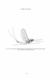
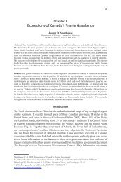
People<br />
Analyses<br />
Hardware<br />
<strong>GIS</strong><br />
Data<br />
S<strong>of</strong>tware<br />
“Our passion for improving quality <strong>of</strong> life<br />
through geography is at the heart <strong>of</strong> everything<br />
we do. Esri's geographic information system<br />
(<strong>GIS</strong>) technology inspires and enables<br />
governments, universities, and businesses<br />
worldwide to save money, lives, and our<br />
environment through a deeper understanding <strong>of</strong><br />
the changing world around them.” Esri, Inc.<br />
Conducting a <strong>GIS</strong> Analysis<br />
In a typical <strong>GIS</strong> analysis project, you need to<br />
first identify the objectives <strong>of</strong> your project,<br />
create a project database containing the data<br />
you need to solve the problem, do any<br />
necessary preprocessing to get the data into<br />
useable format for the task at hand, use <strong>GIS</strong><br />
functions to create an analytical model that<br />
solves the problem, and then interpret and<br />
present your results.<br />
ccn@ualberta.ca 2
<strong>GIS</strong> Project Issues December 2013<br />
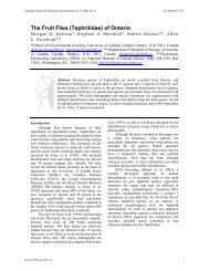
The five <strong>GIS</strong> project steps are as follows:<br />
1. Identify your objectives<br />
2. Assemble a project database<br />
3. Process data for analysis<br />
4. Perform the analysis<br />
5. Present the resulting information<br />
Depending on the type <strong>of</strong> problem you're trying<br />
to solve, this process can be iterative, and <strong>of</strong>ten<br />
the final step leads to more geographic<br />
questions and the whole process begins again.<br />
It is at steps 2 and 3 that can take more time<br />
than necessary if you don’t have the<br />
appropriate skills to import files, work with<br />
various projections, and basically get all your<br />
data “ducks” lined up on a row.<br />
(Attend the spatial referencing and spatial<br />
database development short courses for<br />
instruction on these issues.)<br />
To help get you up to speed on using <strong>GIS</strong><br />
intelligently, there are several <strong>GIS</strong> learning<br />
options available:<br />
U<strong>of</strong>A credit courses: EAS 221, 351,<br />
Biol 471/571, RenR 426, 496<br />
ESRI Online Training:<br />
www.biology.ualberta.ca/facilities/gis/index.<br />
php?Page=484#virtualcampus<br />
<strong>GIS</strong> File Management and S<strong>of</strong>tware<br />
Data used in a <strong>GIS</strong> comes in many forms. Once<br />
in digital form, special care is <strong>of</strong>ten needed<br />
because the usual file management methods<br />
that you may be used to in Windows-based<br />
s<strong>of</strong>tware may corrupt the <strong>GIS</strong> data.<br />
ccn@ualberta.ca 3
<strong>GIS</strong> Project Issues December 2013<br />
ArcCatalog (and selected tools in ArcToolbox)<br />
is the only safe way to rename, copy, and<br />
delete the feature classes and other data<br />
layers. Below are the most common file formats<br />
you will encounter:<br />
A geodatabase is a “container” that stores a<br />
collection <strong>of</strong> datasets as a folder with a name ending<br />
in .gdb (file geodatabase) or .mdb (personal<br />
geodatabase). It is a collection <strong>of</strong> various types <strong>of</strong><br />
<strong>GIS</strong> datasets held in a file system folder and is the<br />
recommended native data format for Arc<strong>GIS</strong> stored<br />
and managed in a file system folder. The vector<br />
datasets are stored as feature classes.<br />
A shapefile is a vector data storage format that<br />
stores the shape and location (*.shp), attributes<br />
(*.dbf), and lookup index (*.shx) <strong>of</strong> geographic<br />
features in a set <strong>of</strong> related files having the same<br />
prefix that must be kept together in the same<br />
directory. Additional files may be present: the very<br />
useful projection definition (*.prj) and spatial index<br />
files (*.sbn) and (*.sbx). When working with<br />
shapefiles, remember to copy all associated files to<br />
the same directory so that they don’t get corrupted!<br />
ArcCatalog will ensure that renaming and<br />
transferring is done properly.<br />
A coverage is a folder-based vector OR raster<br />
(grid) data storage format. A single geographic<br />
theme (such as soils, streams, or land use) is<br />
represented as primary features (such as arcs,<br />
nodes, polygons, and label points OR cells) and<br />
secondary features (such as tics, map extent, links,<br />
and annotation) all stored in a self-named folder.<br />
Associated feature attribute tables describe and<br />
store attributes <strong>of</strong> the geographic features in the info<br />
folder. Use ArcCatalog when copying coverage files<br />
to ensure that the complete data structure is kept<br />
intact.<br />
Note: Grids are coverages.<br />
ccn@ualberta.ca 4
<strong>GIS</strong> Project Issues December 2013<br />
These short courses will focus primarily on the<br />
file geodatabase (*.gdb) format.<br />
www.biology.ualberta.ca/facilities/gis/uploads/in<br />
structions/AVFileTransfer.pdf for more details<br />
on how to transfer <strong>GIS</strong> data so the files don't<br />
corrupt<br />
Arc<strong>GIS</strong> 10 is the latest version <strong>of</strong> desktop <strong>GIS</strong><br />
and mapping s<strong>of</strong>tware developed by<br />
Environmental Systems Research Institute,<br />
Inc. (ESRI) that allows you to visualize, create,<br />
solve, and present spatial data in your<br />
ecological research<br />
ArcMap<br />
Arc<strong>GIS</strong> Desktop refers to a suite <strong>of</strong> scalable<br />
products composed <strong>of</strong> core applications and an<br />
integrated set <strong>of</strong> tools:<br />
ArcMap<br />
Create and interact with maps<br />
View, edit, query relationships, and<br />
analyze geographic data<br />
Standalone application<br />
ArcCatalog<br />
Find, preview, document, and organize<br />
geographic data<br />
View and update metadata<br />
Standalone and dockable inside ArcMap<br />
ArcToolbox<br />
Access form-based <strong>GIS</strong> tools<br />
Projections, conversions, geoprocessing<br />
Dockable inside ArcMap, ArcCatalog<br />
ccn@ualberta.ca 5
<strong>GIS</strong> Project Issues December 2013<br />
ArcCatalog<br />
ArcToolbox<br />
ArcView 10, ArcEditor 10, and ArcInfo 10 are<br />
also called Arc<strong>GIS</strong> Desktop 10 – the user<br />
interfaces are exactly the same but the level <strong>of</strong><br />
functionality and amount <strong>of</strong> analysis tools are<br />
greatest in ArcInfo. For more information see<br />
www.esri.com, and to find out how to get the<br />
s<strong>of</strong>tware for yourself, see<br />
www.biology.ualberta.ca/facilities/gis/index.php<br />
?Page=484#mycomputer.<br />
Course Data Sources<br />
Free spatial data that can be used for <strong>GIS</strong><br />
analysis in ecological applications have been<br />
obtained from the GeoGratis website<br />
http://geogratis.cgdi.gc.ca (Atlas <strong>of</strong> Canada and<br />
EcoAtlas). The following summarizes the<br />
metadata (description) for each geographic<br />
layer in the course dataset that has been made<br />
available to you in the<br />
\\Bio_print\courses\<strong>GIS</strong>-100 directory.<br />
Name<br />
File<br />
Format Description Feature<br />
alberta .shp Province boundary Polygon<br />
ecoatlas .e00 National Ecological<br />
Framework<br />
Polygon<br />
lake .shp Lakes and rivers Polygon<br />
river .shp Rivers and streams Line<br />
road .shp Roads line<br />
place .shp Populated places Point<br />
ccn@ualberta.ca 6
<strong>GIS</strong> Project Issues December 2013<br />
Area: <strong>Alberta</strong><br />
Data Model: Vector<br />
Scale: 1:2,000,000<br />
Projection / Datum: GCS NAD 83<br />
Units: Decimal Degrees<br />
See the course \_documentation folder for<br />
more details on the sources <strong>of</strong> data used.<br />
Tasks<br />
Managing files, exploring the interface <strong>of</strong> the<br />
<strong>GIS</strong> s<strong>of</strong>tware, adding and displaying layers,<br />
symbolizing, and editing layer properties<br />
Copying <strong>GIS</strong> Data<br />
The quantity <strong>of</strong> <strong>GIS</strong> data files <strong>of</strong>ten necessitates<br />
you to utilize the network and/or copy to a disk<br />
or flash drive for storing and transferring the<br />
data needed for your projects.<br />
TIP: Invest in a portable hard drive! But have<br />
a backup!<br />
Windows Explorer and Servers<br />
The data files for the <strong>GIS</strong> short courses in the<br />
BioComputing teaching lab (B118) are located<br />
on the local Bio_print server, accessible via<br />
the Local Area Network (LAN). Use Windows<br />
Explorer to navigate to appropriate directories.<br />
1. Double click on the COURSES shared<br />
directory icon on the Desktop<br />
2. Click on the FOLDERS button (located on<br />
the standard tool bar below the main menu)<br />
– this transforms the window into Windows<br />
Explorer<br />
3. On the left side <strong>of</strong> the exploring window,<br />
click and drag the scroll bar until you can<br />
see “My Computer”<br />
4. Expand “My Computer” by clicking the “+”<br />
5. Expand “Local Disk (C:)” by clicking the “+”<br />
6. In the right side <strong>of</strong> the exploring window,<br />
double click the “<strong>GIS</strong>-100” folder to open it<br />
7. Click and drag (copy and paste) the “0_<strong>GIS</strong>”<br />
folder to the C:\WorkSpace directory<br />
The COURSES directory and all sub-folders<br />
are read only; therefore you cannot modify<br />
the data or store additional files here. Note:<br />
These instructions are for the B118 lab only.<br />
ccn@ualberta.ca 7
<strong>GIS</strong> Project Issues December 2013<br />
8. Open the subdirectories <strong>of</strong><br />
C:\WorkSpace\0_<strong>GIS</strong> to view the various<br />
<strong>GIS</strong> file structures<br />
9. Notice the lack <strong>of</strong> spaces in the folder and<br />
file names!!!<br />
10. Minimize the Explorer window when done<br />
www.biology.ualberta.ca/facilities/gis/uploads/in<br />
structions/MS<strong>GIS</strong>ServerAccess.pdf has<br />
instructions on how to access the Shared_<strong>GIS</strong><br />
server on the Bio-sci network, accessible only<br />
to users within the <strong>Biological</strong> <strong>Sciences</strong> Building.<br />
This is where you can find Arc<strong>GIS</strong> manuals,<br />
store your <strong>GIS</strong> project files, obtain generic data<br />
for study area mapping, and temporarily FTP.<br />
You must be logged into a computer using your<br />
generic lab user ID and password to be able to<br />
access the Shared_<strong>GIS</strong> server.<br />
File Transfer Protocol (FTP)<br />
A File Transfer Protocol program, such as<br />
WinSCP, is a Windows-based application for<br />
transferring files between the local system (your<br />
PC) and a remote system (an FTP site on a<br />
network server). Using WinSCP, you can<br />
connect to another system from your PC,<br />
browse files and folders on both systems, and<br />
transfer files between the systems. Note: U<strong>of</strong>A<br />
networked servers require the SFTP setting.<br />
AUTHENTICATE (B118 Lab) then click START<br />
>>> PROGRAMS >>> <strong>University</strong> <strong>of</strong> <strong>Alberta</strong> >>><br />
WinSCP<br />
If you are unfamiliar with FTP, see<br />
http://helpdesk.ualberta.ca/storage/multimedia/<br />
winscp.<br />
The following information can be used to<br />
transfer files from the PC you are working on in<br />
the lab to an outside server:<br />
Host Name/Address gisserver.biology.ualberta.ca<br />
User ID gis-ftp<br />
Password By request<br />
Note Temporary directories for transferring files that<br />
you may want to copy to a computer outside B118<br />
Host Name/Address gpu.srv.ualberta.ca<br />
User ID Your CCID<br />
Password Your CCID password<br />
Note Your personal directories associated with your<br />
CCID (first half <strong>of</strong> your @ualberta.ca email)<br />
ccn@ualberta.ca 8
<strong>GIS</strong> Project Issues December 2013<br />
Managing Data with ArcCatalog<br />
Using ArcCatalog:<br />
Copying and working with <strong>GIS</strong> data file formats<br />
can easily be accomplished with Arc<strong>GIS</strong>’s<br />
ArcCatalog application. This interface is<br />
designed to flawlessly copy all associated files<br />
required for the data to work properly in the<br />
<strong>GIS</strong>. It works very similar to Windows Explorer<br />
with drag and drop capability!<br />
1. Choose START >>> PROGRAMS >>><br />
ARC<strong>GIS</strong> >>> ARCCATALOG<br />
Make a handy connection to the<br />
C:\WorkSpace\0_<strong>GIS</strong> directory (also applies to<br />
a CD, portable hard drive, or other folder on the<br />
network or local hard drive)<br />
TIP: Do not make connections to every single<br />
subfolder; instead make a few connections to<br />
upper-level key folders <strong>of</strong> your data files<br />
2. Click on the CONNECT TO FOLDER icon<br />
3. Navigate to the appropriate location;<br />
e.g. C:\WorkSpace\0_<strong>GIS</strong><br />
4. Click OK<br />
5. Double click on the \<strong>Alberta</strong>.gdb directory<br />
to view its contents<br />
6. Take a moment to examine the ArcCatalog<br />
window and Main Menu<br />
7. Highlight each <strong>of</strong> the files<br />
8. Click on PREVIEW tab - ArcCatalog<br />
displays the “Geography” <strong>of</strong> the layer<br />
9. Change the Preview: from “Geography” to<br />
“Table” and examine it<br />
ccn@ualberta.ca 9
<strong>GIS</strong> Project Issues December 2013<br />
This is the attribute table associated with the<br />
layer and looks remarkably like an MS Access<br />
database table!<br />
10. Click on the DESCRIPTION tab<br />
11. Double click the \Shapefiles and<br />
\Coverages directories to repeat your visual<br />
investigation <strong>of</strong> the data<br />
12. select and examine the distinct file structure<br />
by viewing in both ArcCatalog and Windows<br />
Explorer<br />
NOTE: The coverages, shapefiles and feature<br />
classes appear as single files in the ArcCatalog<br />
window – but not in Windows Explorer. What<br />
colour icon is used for each vector file?<br />
Accessing Arc<strong>GIS</strong> Desktop Help:<br />
To find out more about metadata, or anything<br />
else in Arc<strong>GIS</strong>, take advantage <strong>of</strong> the wonderful<br />
Arc<strong>GIS</strong> Desktop Help. This built-in help system<br />
can be accessed from ArcCatalog and ArcMap.<br />
Help is also on-line anytime anywhere:<br />
http://help.arcgis.com/en/arcgisdesktop/10.0/help/<br />
13. Choose HELP >>> ARC<strong>GIS</strong> DESKTOP<br />
HELP<br />
14. Click on each <strong>of</strong> the tabs to see what they<br />
contain<br />
15. Click on the SEARCH tab<br />
16. Type in “metadata” as the keyword to find<br />
17. Select “What is metadata?” in the topic list<br />
18. Take a quick look at the help file dialog<br />
19. Click on the CONTENTS tab<br />
Make note <strong>of</strong> which topics to peruse later at<br />
your leisure to learn as much as you can about<br />
the importance <strong>of</strong> metadata, and then close the<br />
window. Notice that Arc<strong>GIS</strong> has several<br />
features for examining and managing your<br />
geographic layers, and there are excellent<br />
resources on <strong>GIS</strong> fundamentals inside the<br />
s<strong>of</strong>tware’s help files!<br />
20. CLOSE the help system<br />
Launching ArcMap:<br />
21. Click on the LAUNCH ARCMAP<br />
button in ArcCatalog<br />
22. Start using ArcMap with a new empty map<br />
and click OK<br />
23. CLOSE ArcCatalog<br />
ccn@ualberta.ca 10
<strong>GIS</strong> Project Issues December 2013<br />
ArcMap and Map Documents<br />
Take a moment to examine the ArcMap window<br />
and look through the MA<strong>IN</strong> MENU. ArcMap<br />
displays geographic information as layers, and<br />
each layer represents a particular type <strong>of</strong><br />
feature such as populated places, rivers, lakes,<br />
or wildlife habitat. The references (NOT the<br />
actual data files) to these layers are stored in<br />
the map document (.mxd file).<br />
Several toolbars are available for you to point<br />
and click your way through the displaying <strong>of</strong><br />
layers and performing <strong>GIS</strong> functions on them.<br />
Select which toolbars you need from the<br />
CUSTOMIZE > >> TOOLBARS pull-down menu<br />
or choose CUSTOMIZE >>> CUSTOMIZE<br />
MODE and check each in the TOOLBARS tab.<br />
The table <strong>of</strong> contents lists all the layers on the<br />
map and indicates what the features in each<br />
layer represent. Turn it on or <strong>of</strong>f via W<strong>IN</strong>DOWS<br />
>>> TABLE OF CONTENTS. The order in<br />
which layers are drawn depends on their<br />
positions within the table <strong>of</strong> contents; the layer<br />
at the top draws over the one below. LIST BY<br />
DRAW<strong>IN</strong>G ORDER, LIST BY SOURCE, LIST<br />
BY VISIBILITY, and LIST BY SELECTION help<br />
manage layers.<br />
Again, the layers in the table <strong>of</strong> contents are<br />
the references to feature classes, shapefiles,<br />
coverages, grids, images, etc. that you add to<br />
the map document. You can modify the drawing<br />
order, turn them on and <strong>of</strong>f , and expand<br />
or collapse their legends. Layers are<br />
organized into data frames , which simply<br />
group the layers that you want to display<br />
together. The default data frame name is<br />
“Layers.” You can add more than one data<br />
ccn@ualberta.ca 11
<strong>GIS</strong> Project Issues December 2013<br />
frame when comparing layers side by side or<br />
for creating map insets and overviews. When<br />
there is more than one data frame in the map,<br />
only one <strong>of</strong> them is the active data frame (i.e.<br />
the one you're currently working with is<br />
highlighted on the map and shown in bold text<br />
in the table <strong>of</strong> contents). When you add a new<br />
layer to a map, it is added to the active data<br />
frame.<br />
Layers and data frames have properties<br />
associated with them that you can edit and<br />
modify according to how you want the data to<br />
be displayed. You control all aspects <strong>of</strong> a layer<br />
through the layer properties by defining how it<br />
is drawn, the source <strong>of</strong> its data, what gets<br />
labeled, attribute field properties, etc. You can<br />
customize the data frame name, position,<br />
coordinate system, grid, map and display units,<br />
appearance, etc. through data frame<br />
properties. Access the properties by right<br />
clicking on the layer or data frame and clicking<br />
on PROPERTIES or simply by double clicking<br />
on the name.<br />
Depending on how you want to look at and<br />
interact with your geographic information,<br />
ArcMap provides you with<br />
two different ways to view<br />
your map. Use data view<br />
when you want to browse<br />
the geographic data on your<br />
map or perform analyses on layers specific to<br />
the data frame. Use layout view when you’re<br />
preparing your map for presentation to an<br />
audience. You can switch between views<br />
through the VIEW pull-down menu or by<br />
clicking the view buttons found in the lower left<br />
portion <strong>of</strong> the display window.<br />
Setting up the ArcMap working<br />
environment:<br />
1. Click on each <strong>of</strong> the headings in the MA<strong>IN</strong><br />
MENU to view what’s available<br />
2. Choose CUSTOMIZE >>> TOOLBARS<br />
3. Make sure there is a check beside the<br />
following toolbars:<br />
Standard<br />
Tools<br />
Draw<br />
Layout<br />
4. Click and drag each toolbar so that they are<br />
positioned as you like<br />
ccn@ualberta.ca 12
<strong>GIS</strong> Project Issues December 2013<br />
5. Right click anywhere on the MA<strong>IN</strong> MENU to<br />
view the TOOLBARS listing<br />
6. Remove the LAYOUT toolbar by clicking on<br />
the check mark<br />
7. Hover the mouse cursor over each <strong>of</strong> the<br />
buttons on the toolbars to read the tool tip –<br />
the status bar at the lower left provides<br />
more details<br />
Adding data layers:<br />
8. Click on the ADD DATA button<br />
9. Navigate to the<br />
C:\WorkSpace\0_<strong>GIS</strong>\<strong>Alberta</strong>.gdb<br />
directory<br />
10. Select ALL layers by holding the SHIFT key<br />
and clicking on the first and last files in the<br />
\<strong>Alberta</strong>.gdb directory<br />
11. Click ADD<br />
TIP: Holding the CTRL or SHIFT key enables<br />
multiple file selections!<br />
Turning layers on and <strong>of</strong>f:<br />
12. In the table <strong>of</strong> contents, click on the check<br />
box beside river to turn it OFF<br />
13. Turn OFF the rest <strong>of</strong> the layers by clicking in<br />
their check boxes<br />
14. Hold the CTRL key and click in any <strong>of</strong> the<br />
empty check boxes to turn on all layers at<br />
the same time (The same CTRL key<br />
technique works for turning them all <strong>of</strong>f,<br />
too.)<br />
The drawing order <strong>of</strong> layers:<br />
The order <strong>of</strong> layers listed in the table <strong>of</strong><br />
contents determines how layers are drawn on a<br />
map. Within a data frame, the layers listed at<br />
the top will draw over those listed below them,<br />
and so on down the list. You can easily move<br />
layers around to adjust their drawing order or<br />
organize them in separate data frames. For<br />
example, roads should be drawn over rivers.<br />
15. Make sure all data layers are turned ON<br />
16. Click and drag lake up until a black line<br />
indicates that the layer will be placed above<br />
river<br />
17. Move the place layer so it draws on top <strong>of</strong><br />
all other layers – points default to this<br />
location<br />
18. Position the remaining layers appropriately;<br />
i.e. road above river<br />
ccn@ualberta.ca 13
<strong>GIS</strong> Project Issues December 2013<br />
Viewing data frame and layer<br />
properties:<br />
19. Right-click on the data frame entitled<br />
“Layers”<br />
20. Click PROPERTIES – alternately, choose<br />
VIEW >>> DATA FRAME PROPERTIES<br />
21. Click on each <strong>of</strong> the tabs to see what they<br />
contain<br />
22. Select the GENERAL tab<br />
23. Change the name <strong>of</strong> the data frame to<br />
“<strong>Alberta</strong>”<br />
24. Click OK to apply the change and close the<br />
window<br />
25. Right click on the river layer<br />
26. Click on PROPERTIES<br />
27. Click on each <strong>of</strong> the tabs to see what they<br />
contain<br />
28. CLOSE the window<br />
Adding a new data frame:<br />
29. Choose <strong>IN</strong>SERT >>> DATA FRAME<br />
30. Right-click “New Data Frame”<br />
31. Click on ADD DATA…<br />
32. Navigate to the \Shapefiles folder to select<br />
ALL the layers<br />
33. Click ADD<br />
34. Repeat for the \Coverages folder<br />
The most complex layer (polygon or annotation)<br />
is added for the coverage.<br />
35. Click once on the name “New Data Frame”<br />
to highlight it<br />
36. Wait a moment and then click it again to<br />
access the text box<br />
37. Change the name <strong>of</strong> the data frame by<br />
typing “<strong>Alberta</strong> Shapes” and press ENTER<br />
Removing a layer from the data<br />
frame:<br />
38. Right click on any layer and click REMOVE<br />
Switching between data frames:<br />
When in data view, you can see only one data<br />
frame. You cannot see both data frames at the<br />
same time unless you switch to layout view to<br />
create a map (subject <strong>of</strong> a future short<br />
course).The active data frame name will<br />
appear in bolded text in the table <strong>of</strong> contents.<br />
39. Right-click on the data frame entitled<br />
“<strong>Alberta</strong>”<br />
40. Click ACTIVATE – you are now looking at<br />
that data frame<br />
ccn@ualberta.ca 14
<strong>GIS</strong> Project Issues December 2013<br />
41. Hold the ALT key and click on the “<strong>Alberta</strong><br />
Shapes” data frame – shortcut to activate<br />
42. Click on the “-“ next to “<strong>Alberta</strong> Shapes” to<br />
collapse its legend<br />
43. Switch back to (activate) the “<strong>Alberta</strong>” data<br />
view<br />
44. Remove the “<strong>Alberta</strong> Shapes” data frame<br />
Saving your map document:<br />
First set the map document properties.<br />
45. Choose FILE >>> MAP DOCUMENT<br />
PROPERTIES<br />
46. Check “Store relative pathnames to data<br />
sources” and click OK<br />
47. Choose FILE >>> SAVE AS<br />
48. Navigate to the C:\WorkSpace\0_<strong>GIS</strong><br />
directory<br />
49. Type a name; e.g.<br />
<strong>Alberta</strong>_todaysdate.mxd<br />
50. Click SAVE<br />
IMPORTANT TIP: relative path names specify<br />
the location <strong>of</strong> the map data relative to the<br />
current location on disk <strong>of</strong> the map document<br />
(.mxd file) itself. Since relative paths don't<br />
contain drive names (e.g. C:\Workspace), they<br />
make it easier for you to move the map and its<br />
associated data to any disk drive without the<br />
map having to be repaired. As long as the same<br />
directory structure is used at the new location<br />
(e.g. \0_<strong>GIS</strong>), the map will still be able to find its<br />
data by traversing the relative paths.<br />
Symbolizing Your Data<br />
This section demonstrates how you can<br />
communicate specific attributes <strong>of</strong> geographic<br />
information to your map audience. ArcMap has<br />
several ways to spruce up legend styles to<br />
make your map look more visually appealing<br />
and convey more meaningful information.<br />
Point symbology:<br />
1. Turn OFF all layers in the “<strong>Alberta</strong>” data<br />
frame and turn ON place<br />
2. Click on the SYMBOL for place<br />
Clicking directly on the symbol patch is a<br />
shortcut for modifying its properties.<br />
3. Scroll through the various point symbols to<br />
choose one and modify the color/size<br />
4. Click OK<br />
ccn@ualberta.ca 15
<strong>GIS</strong> Project Issues December 2013<br />
5. In the table <strong>of</strong> contents, change the place<br />
layer name to “Towns”<br />
6. Make a copy <strong>of</strong> the place layer:<br />
Right click on the “Towns” layer NAME<br />
<br />
and choose COPY LAYER<br />
Right click on the “<strong>Alberta</strong>” data frame<br />
NAME and choose PASTE LAYER(S)<br />
There are several ways to symbolize points,<br />
especially if the point layer has attributes<br />
associated with them.<br />
7. Double click on the new “Towns” layer<br />
NAME to view its properties<br />
8. Select the SYMBOLOGY tab<br />
9. Show QUANTITIES as GRADUATED<br />
SYMBOLS<br />
10. Specify POP91 as the Value Field<br />
11. Accept all defaults<br />
You will get practice with various classification<br />
options when symbolizing polygons.<br />
12. Change the layer name in the GENERAL<br />
tab to “Populations” and click OK<br />
Line symbology:<br />
13. Turn OFF all layers in the “<strong>Alberta</strong>” data<br />
frame and turn ON river and road<br />
14. Double click on the NAME for river<br />
15. Click on the SYMBOLOGY tab in the Layer<br />
Properties window<br />
16. Click on the symbol button<br />
17. Select the RIVER symbol<br />
18. Click OK twice<br />
ArcMap has several <strong>of</strong> these preset symbol<br />
styles for common geographic features that you<br />
can take advantage <strong>of</strong> for efficient<br />
symbolization!<br />
19. Give the layer a new name under the<br />
GENERAL tab; e.g. “Rivers”<br />
20. Click OK<br />
21. Double click on the road layer name<br />
22. In the Layer Properties window, draw<br />
Categories using TYPE as the Unique<br />
Value<br />
23. Click ADD ALL VALUES<br />
24. Remove the check beside <br />
25. Double-click on each <strong>of</strong> the line symbols<br />
and give them an appropriate color/style<br />
26. In the GENERAL tab, change the layer<br />
name to “Roads”<br />
27. Click OK<br />
Just as when symbolizing points, you may use<br />
attributes associated with line layers to<br />
symbolize them effectively.<br />
ccn@ualberta.ca 16
<strong>GIS</strong> Project Issues December 2013<br />
Polygon features are used in the following<br />
examples to familiarize you with the subtleties<br />
<strong>of</strong> data classification.<br />
Keep in mind that the value classification<br />
schemes may be applied to all features (points,<br />
lines, polygons) and raster data, too, that have<br />
numeric attribute values. Data classification is<br />
similar to ‘binning’ in statistical s<strong>of</strong>tware, only<br />
you get a visual representation!<br />
Deciding on an attribute to map:<br />
1. View \0_<strong>GIS</strong>\_documentation\<br />
ecoatlas_descriptions.xls<br />
2. Read the descriptions <strong>of</strong> the various<br />
attributes and select one; e.g. BIRDS<br />
(number <strong>of</strong> terrestrial bird species) – this is<br />
a good example to use because you can<br />
experiment with normalizing the counts by<br />
area<br />
3. Turn all layers OFF and turn ON ecoatlas<br />
4. COLLAPSE all other layers’ symbols and<br />
EXPAND ecoatlas<br />
5. Double click on the ecoatlas NAME to<br />
access its PROPERTIES<br />
6. Show CATEGORIES as a Unique Values<br />
and select BIRDS as the Value Field<br />
7. Click OK<br />
8. View the resulting map <strong>of</strong> values<br />
Symbolizing using the default<br />
classification:<br />
9. Double click on the ecoatlas NAME to<br />
access its PROPERTIES<br />
10. In the SYMBOLOGY tab, show<br />
QUANTITIES using Graduated Colors<br />
11. Select BIRDS as the VALUE using the<br />
default classification (5 Natural Breaks)<br />
12. Click OK<br />
13. View the resulting map<br />
Exploring the classification<br />
histogram:<br />
14. Double click on the ecoatlas NAME to<br />
access its PROPERTIES<br />
15. In the SYMBOLOGY tab, click<br />
on the CLASSIFY button<br />
16. Click a check in the “Show Std. Dev.”<br />
And “Show Mean” check boxes<br />
17. Examine the classification statistics, break<br />
values, and frequency distribution<br />
ccn@ualberta.ca 18
<strong>GIS</strong> Project Issues December 2013<br />
Changing the classification method<br />
to equal interval:<br />
18. Select Equal Interval from the classification<br />
method drop-down box<br />
19. Maintain the 5 classes<br />
20. Take note <strong>of</strong> the break values<br />
21. Click OK<br />
22. Click APPLY<br />
23. View the resulting map<br />
24. Position the Layer Properties window so<br />
you can see both it and the ecoatlas layer<br />
in the data view<br />
Changing the classification method<br />
to quantile:<br />
25. Return to the SYMBOLOGY tab and click<br />
the CLASSIFY button<br />
26. Select Quantile from the classification<br />
method drop-down box<br />
27. Maintain the 5 classes<br />
28. Take note <strong>of</strong> the break values<br />
29. Click OK<br />
30. Click APPLY<br />
31. View the resulting map<br />
Changing the classification method<br />
to standard deviation:<br />
32. Return to the SYMBOLOGY tab and click<br />
the CLASSIFY button<br />
33. Select Standard Deviation from the<br />
classification method drop-down box<br />
34. Keep 1 Std Dev as the interval<br />
35. Take note <strong>of</strong> the break values<br />
36. Click OK<br />
37. Click APPLY<br />
38. View the resulting map<br />
Specifying your own class breaks:<br />
39. Return to the SYMBOLOGY tab and click<br />
the CLASSIFY button<br />
40. Select Manual from the classification<br />
method drop-down box<br />
41. Select 5 classes<br />
42. Type new numbers or reposition the<br />
histogram break bars to set new break<br />
values<br />
43. Click OK<br />
44. Click APPLY<br />
45. View the resulting map<br />
ccn@ualberta.ca 19
<strong>GIS</strong> Project Issues December 2013<br />
Normalizing the data:<br />
Create ratios, by dividing two data values, if you<br />
want to minimize differences based on the size<br />
<strong>of</strong> areas or number <strong>of</strong> features in each area –<br />
also referred to as normalizing the data.<br />
46. Return to the SYMBOLOGY tab and click<br />
the CLASSIFY button<br />
47. Select Natural Breaks from the<br />
classification method drop-down box<br />
48. Maintain the 5 classes<br />
49. Click OK<br />
50. Select AREAKM in the Normalization dropdown<br />
box<br />
51. Click APPLY<br />
52. View the resulting map<br />
48. Experiment with the different classification<br />
methods on the normalized data – you<br />
should notice very different distribution<br />
patterns from the original count data<br />
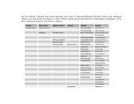
View the table below, statistical textbooks, and<br />
SEARCH the online help for “classification<br />
schemes”: examine several <strong>of</strong> the topics.<br />
METHOD WHEN TO USE NUMBER CLASSES<br />
Natural<br />
Breaks<br />
Equal<br />
Interval<br />
Quantile<br />
Standard<br />
Deviation<br />
Attributes are<br />
distributed<br />
unevenly across<br />
the overall range<br />
<strong>of</strong> values<br />
All classes should<br />
have the same<br />
range<br />
Attributes are<br />
distributed evenly<br />
distribution across<br />
the range <strong>of</strong><br />
values<br />
Show how much a<br />
feature’s attribute<br />
value varies from<br />
the mean<br />
Choose a number that<br />
best reflects the natural<br />
groups <strong>of</strong> attributes you<br />
want to show<br />
Choose a number that<br />
produces an easily<br />
understood interval (2,<br />
50, 1000, etc.) or, the<br />
number <strong>of</strong> classes that<br />
produces a map with<br />
your intended message<br />
Choose a number that<br />
makes sense for the<br />
purpose <strong>of</strong> your map<br />
Choose the interval size<br />
(1/3 to 1 std dev and<br />
ArcMap calculates the<br />
mean value and the<br />
standard deviations<br />
from the mean to use in<br />
creating class breaks<br />
For additional symbology tips/guidelines, see<br />
the companion slides at<br />
www.biology.ualberta.ca/facilities/gis/?Page=485<br />
ccn@ualberta.ca 20
<strong>GIS</strong> Project Issues December 2013<br />
Saving layer (*.lyr) files:<br />
You can save everything about the layer<br />
(symbology, labels, classification) in a layer file<br />
(*.lyr). This is very convenient because when<br />
the layer file gets added to another map<br />
document, it references the shapefile and tells<br />
ArcMap to draw it exactly as it was saved. Now<br />
whenever you wish to display this layer, add the<br />
*.lyr file instead the original data.<br />
49. Right click on Roads and click SAVE AS<br />
LAYER FILE<br />
50. Specify a directory location and name and<br />
click SAVE<br />
Repeat making *.lyr files for other layers you<br />
symbolized. Now whenever you wish to display<br />
this layer in a new map document, add the *.lyr<br />
file instead the original data.<br />
51. Choose <strong>IN</strong>SERT >>> NEW DATA FRAME<br />
52. Click the ADD DATA button and add some<br />
<strong>of</strong> these *.lyr files and their corresponding<br />
data sources; e.g. Roads.lyr and road.shp<br />
Now What?<br />
When you are finished working with your data,<br />
always securely store and make a backup <strong>of</strong><br />
your files. The example here has all data layers<br />
stored in a single main directory/folder: 0_<strong>GIS</strong>.<br />
The map document properties were set to store<br />
relative path names. You should copy the entire<br />
folder to another disk, server, or external drive.<br />
You may also zip the entire folder and email as<br />
an attachment.<br />
53. SAVE the map document and CLOSE when<br />
done<br />
54. Try out the instructions above on File<br />
Transfer Protocol (FTP)<br />
55. Use Windows Explorer to COPY to an<br />
external storage device<br />
ccn@ualberta.ca 21