PRACTICAL ACTIVITIES
PRACTICAL ACTIVITIES PRACTICAL ACTIVITIES
PRACTICAL ACTIVITIES A ‘Striking’ Demonstration of the Poisson Distribution Oxford, TEST Teaching 0141-982X © 26 3Practical Blackwell UK Activities Statistics Publishing, Ltd. 2004 KEYWORDS: Teaching; Intellectual excitement; Long-term learning; Poisson demonstration. Vincent Buonaccorsi and Amy Skibiel Juniata College, Huntingdon, Pennsylvania, USA. e-mail: buonaccorsi@juniata.edu Summary This article describes a simple classroom activity that helps students immediately visualize and understand the meaning and mathematical properties of the Poisson distribution. INTRODUCTION Striking interactive demonstrations add excitement to teaching and learning statistics (Sowey 2001), improve statistical intuition (Shaughnessy 1992) and may enhance long-term learning (Sowey 2001). Without illustration or first-hand experience, probability distributions may remain abstract theoretical constructs in an introductory statistics class. To give students experience in using the Poisson distribution, plot-sampling methods for plants or animals may be used to determine whether a distribution is random, clumped or uniform (e.g. Brower et al. 1997). However, such methods are typically time intensive, and may require a laboratory section or specialized equipment. Here we describe a simple interactive demonstration that was successfully used for two years in an undergraduate biostatistics lecture setting. The demonstration immediately and clearly illustrated the Poisson distribution, and a student survey (n = 7, self selection) indicated strong agreement that the activity had educational value and should be kept in future years. A Poisson distribution of split peas per sampling quadrat was generated as a student dropped a handful of split peas onto a grid that was projected on an overhead projector. Data analysis consisted of (1) tallying the observed frequencies of peas per quadrat, (2) calculating the mean number of peas per quadrat, (3) calculating the Poisson estimated probabilities for each outcome, (4) calculating the Poisson expected frequencies, (5) calculating and comparing the mean and variance of the distribution, (6) calculating the coefficient of dispersion (CD) and (7) evaluating the fit of observed and expected frequencies using a chi-square goodnessof-fit test. CONSTRUCTION OF GRID A 20 cm × 20 cm grid comprised of one hundred 2 cm 2 quadrats was drawn with a permanent marker on a transparency and taped to a 36 cm by 36 cm cardboard box lid (figure 1). The grid was placed directly over a 20 cm × 20 cm square cutout in the centre of the box lid to allow the grid to be visualized Fig 1. 8 • Teaching Statistics. Volume 27, Number 1, Spring 2005
- Page 2 and 3: on a screen using an overhead proje
<strong>PRACTICAL</strong> <strong>ACTIVITIES</strong><br />
A ‘Striking’ Demonstration of the Poisson Distribution<br />
Oxford, TEST Teaching 0141-982X © 26 3Practical Blackwell UK Activities Statistics Publishing, Ltd. 2004<br />
KEYWORDS:<br />
Teaching;<br />
Intellectual excitement;<br />
Long-term learning;<br />
Poisson demonstration.<br />
Vincent Buonaccorsi and Amy Skibiel<br />
Juniata College, Huntingdon, Pennsylvania, USA.<br />
e-mail: buonaccorsi@juniata.edu<br />
Summary<br />
This article describes a simple classroom activity<br />
that helps students immediately visualize and understand<br />
the meaning and mathematical properties of<br />
the Poisson distribution.<br />
INTRODUCTION <br />
Striking interactive demonstrations add excitement<br />
to teaching and learning statistics (Sowey<br />
2001), improve statistical intuition (Shaughnessy<br />
1992) and may enhance long-term learning (Sowey<br />
2001). Without illustration or first-hand experience,<br />
probability distributions may remain abstract<br />
theoretical constructs in an introductory statistics<br />
class. To give students experience in using the<br />
Poisson distribution, plot-sampling methods for<br />
plants or animals may be used to determine<br />
whether a distribution is random, clumped or<br />
uniform (e.g. Brower et al. 1997). However, such<br />
methods are typically time intensive, and may<br />
require a laboratory section or specialized equipment.<br />
Here we describe a simple interactive demonstration<br />
that was successfully used for two years in<br />
an undergraduate biostatistics lecture setting. The<br />
demonstration immediately and clearly illustrated<br />
the Poisson distribution, and a student survey<br />
(n = 7, self selection) indicated strong agreement<br />
that the activity had educational value and should<br />
be kept in future years.<br />
A Poisson distribution of split peas per sampling<br />
quadrat was generated as a student dropped a<br />
handful of split peas onto a grid that was projected<br />
on an overhead projector. Data analysis consisted<br />
of (1) tallying the observed frequencies of peas per<br />
quadrat, (2) calculating the mean number of peas<br />
per quadrat, (3) calculating the Poisson estimated<br />
probabilities for each outcome, (4) calculating the<br />
Poisson expected frequencies, (5) calculating and<br />
comparing the mean and variance of the distribution,<br />
(6) calculating the coefficient of dispersion<br />
(CD) and (7) evaluating the fit of observed and<br />
expected frequencies using a chi-square goodnessof-fit<br />
test.<br />
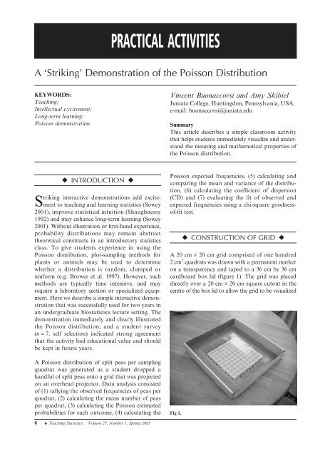
CONSTRUCTION OF GRID <br />
A 20 cm × 20 cm grid comprised of one hundred<br />
2 cm 2 quadrats was drawn with a permanent marker<br />
on a transparency and taped to a 36 cm by 36 cm<br />
cardboard box lid (figure 1). The grid was placed<br />
directly over a 20 cm × 20 cm square cutout in the<br />
centre of the box lid to allow the grid to be visualized<br />
Fig 1.<br />
8 • Teaching Statistics. Volume 27, Number 1, Spring 2005
on a screen using an overhead projector. The grid<br />
covered approximately one half of the lid area,<br />
allowing enough space between the transparency<br />
and lid edges to prevent split peas, dropped from<br />
a height of one foot, from hitting lid edges and<br />
rebounding onto the grid. The lid edges also prevented<br />
peas from falling onto the floor, facilitating<br />
clean-up.<br />
PROCEDURE <br />
At the beginning of the semester, each student in<br />
the class received a numbered syllabus. In class,<br />
a number was drawn using a random numbers<br />
table and the student with that number on his/her<br />
syllabus was selected. This student dropped 150<br />
pre-counted split peas from a height of one foot<br />
above the centre of the grid that had been placed<br />
on an overhead projector. Split peas were used in<br />
the experiment because they are small relative to<br />
quadrat size (maximum possible number of peas/<br />
quadrat is about 20) and they do not roll. Peas<br />
that landed on the border between quadrats were<br />
pushed into the quadrat containing the largest<br />
fraction of the pea area. If it was too difficult to<br />
determine which quadrat contained the largest<br />
fraction of the pea area, the pea was removed from<br />
the grid and not counted in the experiment.<br />
RESULTS AND DISCUSSION <br />
Results from the Fall 2002 semester are presented<br />
(table 1). Approximately half of the peas landed on<br />
the grid. In contrast to what one might expect in a<br />
uniform or clumped distribution, most quadrats<br />
had no peas, some quadrats had one pea, and a few<br />
quadrats had two or three peas (table 1). Estimated<br />
Poisson probabilities were calculated for each<br />
observation category, using the equation<br />
px ( ) =<br />
i<br />
i<br />
x e<br />
x !<br />
where the mean number of peas per quadrat, x<br />
(0.77), was calculated as the total number of peas<br />
observed (77) divided by the number of quadrats<br />
sampled (100), and x i refers to the number of peas<br />
per quadrat. To avoid confusion in calculation of<br />
the mean, it was emphasized that sample size in<br />
this case refers to the total number of units of space<br />
or time (i.e. quadrats), rather than the number of<br />
peas that fell onto the grid. The probability for the<br />
tail of the distribution was calculated as 1 − the sum<br />
of the previous probabilities. Poisson frequencies<br />
were then obtained by multiplying the sample size<br />
(100) by the estimated probabilities.<br />
The Poisson distribution is a probability distribution<br />
of the number of times a random event occurs.<br />
In this experiment the observed frequencies were<br />
close to the probabilities predicted by a Poisson<br />
distribution (table 1).<br />
The coefficient of dispersion (variance/mean)<br />
can be used to determine whether occurrences of<br />
an event are approximately random (CD ≈ 1),<br />
clumped (CD > 1), or uniform (CD < 1) (Sokal<br />
and Rohlf 1995). From a biological viewpoint,<br />
schooling organisms (for example skipjack tuna)<br />
may exhibit clustered distributions whereas territorial<br />
competitive organisms may exhibit uniform or<br />
repulsed distributions (for example sea anemones).<br />
In this experiment, the sample variance (0.68) was<br />
similar to the mean (0.77), yielding a CD of 0.89,<br />
and a reasonable fit of observed frequencies of peas<br />
per quadrat to a Poisson (random) distribution.<br />
However, without a statistical test it is difficult to<br />
interpret whether deviations from Poisson expectations<br />
are due to chance alone.<br />
To determine whether the deviation of observed<br />
frequencies from Poisson expected frequencies was<br />
unlikely to be due to chance alone, a chi-square<br />
x<br />
i<br />
−x<br />
Peas/quadrat<br />
Frequency<br />
(number of quadrats)<br />
Number of<br />
peas observed<br />
Poisson<br />
probabilities<br />
Poisson frequency<br />
(number of quadrats)<br />
0 45 0 0.463 46.3<br />
1 36 36 0.357 35.7<br />
2 16 32 0.137 13.7<br />
3 3 9 0.035 3.5<br />
≥4 0 0 0.008 0.8<br />
Σ = 100 Σ = 77<br />
Table 1. Observed frequencies of peas per quadrat, total number of peas observed per category, estimated Poisson probabilities<br />
and expected Poisson frequencies<br />
Teaching Statistics. Volume 27, Number 1, Spring 2005 • 9
Peas/quadrat<br />
Observed<br />
frequency<br />
Poisson<br />
expected frequency<br />
0 45 46.3<br />
1 36 35.7<br />
≥2 19 18.0<br />
Table 2. Observed and expected Poisson frequencies for each<br />
observation category<br />
goodness-of-fit test was performed. In this experiment,<br />
the observation category of ≥4 peas per<br />
quadrat was lumped with the 2 and 3 peas per<br />
quadrat categories, following the suggestion for<br />
chi-square analysis that no expected frequency<br />
can be less than five (e.g. Sokal and Rohlf 1995).<br />
A chi-square goodness-of-fit test did not detect<br />
a significant difference between observed pea<br />
frequencies and expected Poisson frequencies,<br />
suggesting that the peas followed a Poisson distribution<br />
(table 2, X 2 test statistic = 0.095, p = 0.76). In<br />
other words, the difference between observed and<br />
Poisson expected frequencies was small enough to<br />
be attributable to chance alone.<br />
The following assessment questions have been<br />
used for class discussion and examinations.<br />
1. If a piece of double-sided tape was placed on<br />
the grid, how would you expect it to affect the<br />
CD of the distribution of peas per quadrat?<br />
2. If the mean were 0.5 peas per quadrat, how<br />
many empty quadrats would you expect?<br />
3. How would you expect the mean, variance and<br />
CD of the distribution of peas per quadrat to<br />
change if we increased the number of peas<br />
dropped from 150 to 175, assuming the distribution<br />
is still Poisson?<br />
4. Suppose that every pea landed in a random<br />
fashion and stayed on the grid. How many peas<br />
would have to be dropped to ensure that not<br />
more than 1% of the quadrats remained empty<br />
(adapted from Hampton 1994)?<br />
Acknowledgements<br />
Special thanks to toddler Max Hosler for throwing<br />
a handful of split peas at VPB, Jeff Demarest for<br />
supporting this project, and Randy Bennett for<br />
useful discussion.<br />
References<br />
Brower, J.E., Zar, J.H. and von Ende, C.N.<br />
(1997). Field and Laboratory Methods for<br />
General Ecology. New York, NY: McGraw-<br />
Hill.<br />
Hampton, R.E. (1994). Introductory Biological<br />
Statistics. New York: McGraw-Hill.<br />
Shaughnessy, J.M. (1992). Research in probability<br />
and statistics: reflections and directions.<br />
In: D.A. Grouws (ed.), Handbook<br />
of Research on Mathematics Teaching and<br />
Learning, pp. 465–94. New York: Macmillan.<br />
Sokal, R.R. and Rohlf, F.J. (1995). Biometry.<br />
New York, NY: Freeman.<br />
Sowey, E.R. (2001). Striking demonstrations<br />
in teaching statistics. Journal of Statistics<br />
Education, 9(1).<br />
10 • Teaching Statistics. Volume 27, Number 1, Spring 2005


