Exercise 1 1a) Try help kaiserord to get started. Beware that the ...
Exercise 1 1a) Try help kaiserord to get started. Beware that the ...
Exercise 1 1a) Try help kaiserord to get started. Beware that the ...

Create successful ePaper yourself
Turn your PDF publications into a flip-book with our unique Google optimized e-Paper software.
Johannes J. Struijk, Signalbehandling, 2004, Lecture 8<br />
<strong>Exercise</strong> 1<br />
<strong>1a</strong>)<br />
<strong>Try</strong> <strong>help</strong> <strong>kaiserord</strong> <strong>to</strong> <strong>get</strong> <strong>started</strong>.<br />
<strong>Beware</strong> <strong>that</strong> <strong>the</strong> Kaiser window method only gives an approximate solution. You may<br />
have <strong>to</strong> increase N by 1 or 2 if <strong>the</strong> specifications are not perfectly met.<br />
The MatLab code:<br />
F = [20 30]; % First frequency band (pass) is 0-20, second band (s<strong>to</strong>p) is 30-50<br />
A = [1 0]; % defining <strong>the</strong> bands as pass and s<strong>to</strong>p respectively<br />
DEV = [0.11 0.01] % -1 dB and –40 dB, <strong>the</strong> FIR filter will use <strong>the</strong> smallest of <strong>the</strong><br />
two for both bands! This means <strong>that</strong> <strong>the</strong> pass band will be over dimensioned.<br />
Fs = 100; % sample frequency<br />
[N,wn,beta,type] = <strong>kaiserord</strong>(F,A,DEV,Fs);<br />
b = fir1(N,wn,type,kaiser(N+1,beta),’noscale’);<br />
1b)<br />
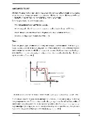
freqz(b,1);<br />
See figure below.<br />
Zooming in at ws=30/50=0.6 shows <strong>that</strong> <strong>the</strong> attenuation is a little more than 40 dB.<br />
Zooming in at wp=20/50=0.4 shows <strong>that</strong> <strong>the</strong> attenuation is much less than <strong>the</strong> allowed<br />
0.11.<br />
The filter thus easily meets <strong>the</strong> requirements.<br />
50<br />
Magnitude (dB)<br />
0<br />
-50<br />
-100<br />
0 0.1 0.2 0.3 0.4 0.5 0.6 0.7 0.8 0.9 1<br />
Normalized Frequency (×π rad/sample)<br />
0<br />
Phase (degrees)<br />
-500<br />
-1000<br />
-1500<br />
0 0.1 0.2 0.3 0.4 0.5 0.6 0.7 0.8 0.9 1<br />
Normalized Frequency (×π rad/sample)<br />
You can use <strong>the</strong> filter <strong>to</strong> filter <strong>the</strong> signal ekg by:<br />
y = filter(b,1,ekg);<br />
1c)<br />
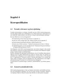
The type of filter can easily be obtained by looking at <strong>the</strong> impulse response:<br />
impz(b,1);
Johannes J. Struijk, Signalbehandling, 2004, Lecture 8<br />
0.6<br />
0.5<br />
0.4<br />
0.3<br />
0.2<br />
0.1<br />
0<br />
-0.1<br />
0 5 10 15 20<br />
The impulse response has an even symmetry and is defined for 0
Johannes J. Struijk, Signalbehandling, 2004, Lecture 8<br />
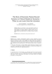
0.5<br />
0.4<br />
0.3<br />
0.2<br />
0.1<br />
0<br />
-0.1<br />
-0.2<br />
-0.3<br />
-0.4<br />
0 2 4 6 8 10 12 14<br />
The impulse response has even symmetry with 0
Johannes J. Struijk, Signalbehandling, 2004, Lecture 8<br />
0.5<br />
0.4<br />
0.3<br />
0.2<br />
0.1<br />
0<br />
-0.1<br />
-0.2<br />
-0.3<br />
-0.4<br />
0 5 10 15 20<br />
3b)<br />
Parks-McClellan<br />
Kaiser<br />
Filter order M = 14 M = 24<br />
S<strong>to</strong>pband ripple equiripple not equiripple<br />
Passband ripple equiripple not equiripple, much better<br />
than <strong>the</strong> specifications<br />
Remez (Parks-McClellan) thus meets <strong>the</strong> specifications with a much lower filter order<br />
than Kaiser.