Chapter 3 Quadratic Programming
Chapter 3 Quadratic Programming
Chapter 3 Quadratic Programming

You also want an ePaper? Increase the reach of your titles
YUMPU automatically turns print PDFs into web optimized ePapers that Google loves.
Optimization I; <strong>Chapter</strong> 3 56<br />
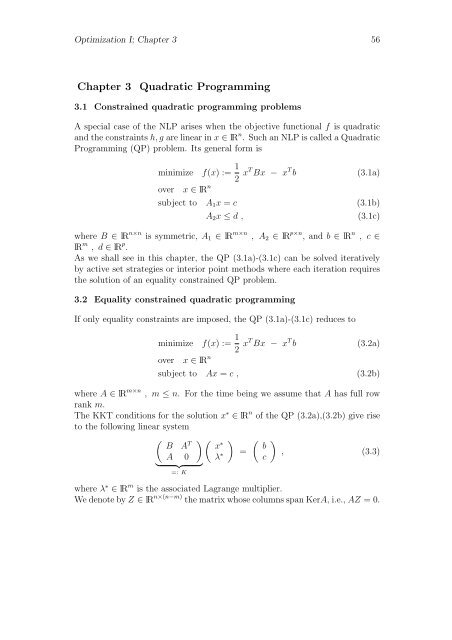
<strong>Chapter</strong> 3 <strong>Quadratic</strong> <strong>Programming</strong><br />
3.1 Constrained quadratic programming problems<br />
A special case of the NLP arises when the objective functional f is quadratic<br />
and the constraints h, g are linear in x ∈ lR n . Such an NLP is called a <strong>Quadratic</strong><br />
<strong>Programming</strong> (QP) problem. Its general form is<br />
minimize f(x) := 1 2 xT Bx − x T b (3.1a)<br />
over<br />
x ∈ lR n<br />
subject to A 1 x = c (3.1b)<br />
A 2 x ≤ d ,<br />
(3.1c)<br />
where B ∈ lR n×n is symmetric, A 1 ∈ lR m×n , A 2 ∈ lR p×n , and b ∈ lR n , c ∈<br />
lR m , d ∈ lR p .<br />
As we shall see in this chapter, the QP (3.1a)-(3.1c) can be solved iteratively<br />
by active set strategies or interior point methods where each iteration requires<br />
the solution of an equality constrained QP problem.<br />
3.2 Equality constrained quadratic programming<br />
If only equality constraints are imposed, the QP (3.1a)-(3.1c) reduces to<br />
minimize f(x) := 1 2 xT Bx − x T b (3.2a)<br />
over<br />
x ∈ lR n<br />
subject to Ax = c , (3.2b)<br />
where A ∈ lR m×n , m ≤ n. For the time being we assume that A has full row<br />
rank m.<br />
The KKT conditions for the solution x ∗ ∈ lR n of the QP (3.2a),(3.2b) give rise<br />
to the following linear system<br />
( B A<br />
T<br />
)<br />
}<br />
A 0<br />
{{ }<br />
=: K<br />
( x<br />
∗<br />
λ ∗ )<br />
=<br />
( b<br />
c<br />
)<br />
, (3.3)<br />
where λ ∗ ∈ lR m is the associated Lagrange multiplier.<br />
We denote by Z ∈ lR n×(n−m) the matrix whose columns span KerA, i.e., AZ = 0.
Optimization I; <strong>Chapter</strong> 3 57<br />
Definition 3.1<br />
KKT matrix and reduced Hessian<br />
The matrix K in (3.3) is called the KKT matrix and the matrix Z T BZ is<br />
referred to as the reduced Hessian.<br />
Lemma 3.2<br />
Existence and uniqueness<br />
Assume that A ∈ lR m×n has full row rank m ≤ n and that the reduced Hessian<br />
Z T BZ is positive definite. Then, the KKT matrix K is nonsingular. Hence,<br />
the KKT system (3.3) has a unique solution (x ∗ , λ ∗ ).<br />
Proof:<br />
The proof is left as an exercise.<br />
Under the conditions of the previous lemma, it follows that the second order<br />
sufficient optimality conditions are satisfied so that x ∗ is a strict local minimizer<br />
of the QP (3.2a),(3.2b). A direct argument shows that x ∗ is in fact a global<br />
minimizer.<br />
Theorem 3.3<br />
Global minimizer<br />
Let the assumptions of Lemma 3.2 be satisfied and let (x ∗ , λ ∗ ) be the unique<br />
solution of the KKT system (3.3). Then, x ∗ is the unique global solution of the<br />
QP (3.2a),(3.2b).<br />
Proof: Let x ∈ F be a feasible point, i.e., Ax = c, and p := x ∗ − x. Then,<br />
Ap = 0. Substituting x = x ∗ − p into the objective functional, we get<br />
f(x) = 1 2 (x∗ − p) T B(x ∗ − p) − (x ∗ − p) T b =<br />
= 1 2 pT Bp − p T Bx ∗ + p T b + f(x ∗ ) .<br />
Now, (3.3) implies Bx ∗ = b − A T λ ∗ . Observing Ap = 0, we have<br />
•<br />
whence<br />
p T Bx ∗<br />
= p T (b − A T λ ∗ ) = p T b − (Ap) T λ ∗ ,<br />
} {{ }<br />
= 0<br />
f(x) = 1 2 pT Bp + f(x ∗ ) .<br />
In view of p ∈ Ker A, we can write p = Zu , u ∈ lR n−m , and hence,<br />
f(x) = 1 2 uT Z T BZu + f(x ∗ ) .<br />
Since Z T BZ is positive definite, we deduce f(x) > f(x ∗ ). Consequently, x ∗ is<br />
the unique global minimizer of the QP (3.2a),(3.2b).<br />
•
Optimization I; <strong>Chapter</strong> 3 58<br />
3.3 Direct solution of the KKT system<br />
As far as the direct solution of the KKT system (3.3) is concerned, we distinguish<br />
between symmetric factorization and the range-space and null-space approach.<br />
3.3.1 Symmetric indefinite factorization<br />
A possible way to solve the KKT system (3.3) is to provide a symmetric factorization<br />
of the KKT matrix according to<br />
P T KP = LDL T , (3.4)<br />
where P is an appropriately chosen permutation matrix, L is lower triangular<br />
with diag(L) = I, and D is block diagonal.<br />
Based on (3.4), the KKT system (3.3) is solved as follows:<br />
( ) b<br />
solve Ly = P T , (3.5a)<br />
c<br />
solve Dŷ = y , (3.5b)<br />
solve L T ỹ = ŷ , (3.5c)<br />
( ) x<br />
∗<br />
set<br />
λ ∗ = P ỹ . (3.5d)<br />
3.3.2 Range-space approach<br />
The range-space approach applies, if B ∈ lR n×n is symmetric positive definite.<br />
Block Gauss elimination of the primal variable x ∗ leads to the Schur complement<br />
system<br />
AB −1 A T λ ∗ = AB −1 b − c (3.6)<br />
with the Schur complement S ∈ lR m×m given by S := AB −1 A T . The rangespace<br />
approach is particularly effective, if<br />
• B is well conditioned and easily invertible (e.g., B is diagonal or blockdiagonal),<br />
• B −1 is known explicitly (e.g., by means of a quasi-Newton updating formula),<br />
• the number m of equality constraints is small.
Optimization I; <strong>Chapter</strong> 3 59<br />
3.3.3 Null-space approach<br />
The null-space approach does not require regularity of B and thus has a wider<br />
range of applicability than the range-space approach.<br />
We assume that A ∈ lR m×n has full row rank m and that Z T BZ is positive<br />
definite, where Z ∈ lR n×(n−m) is the matrix whose columns span Ker A which<br />
can be computed by QR factorization (cf. <strong>Chapter</strong> 2.4).<br />
We partition the vector x ∗ according to<br />
x ∗ = Y w Y + Zw Z , (3.7)<br />
where Y ∈ lR n×m is such that [Y Z] ∈ lR n×n is nonsingular and w Y ∈ lR m , w Z ∈<br />
lR n−m .<br />
Substituting (3.7) into the second equation of (3.3), we obtain<br />
Ax ∗ = AY w Y + }{{} AZ w Z = c , (3.8)<br />
= 0<br />
i.e., Y w Y is a particular solution of Ax = c.<br />
Since A ∈ lR m×n has rank m and [Y Z] ∈ lR n×n is nonsingular, the product<br />
matrix A[Y Z] = [AY 0] ∈ lR m×m is nonsingular. Hence, w Y is well determined<br />
by (3.8).<br />
On the other hand, substituting (3.7) into the first equation of (3.3), we get<br />
BY w Y + BZw Z + A T λ ∗ = b .<br />
Multiplying by Z T and observing Z T A T = (AZ) T = 0 yields<br />
Z T BZw Z = Z T b − Z T BY w Y . (3.9)<br />
The reduced KKT system (3.9) can be solved by a Cholesky factorization of the<br />
reduced Hessian Z T BZ ∈ lR (n−m)×(n−m) . Once w Y and w Z have been computed<br />
as the solutions of (3.8) and (3.9), x ∗ is obtained according to (3.7).<br />
Finally, the Lagrange multiplier turns out to be the solution of the linear system<br />
arising from the multiplication of the first equation in (3.7) by Y T :<br />
(AY ) T λ ∗ = Y T b − Y T Bx ∗ . (3.10)<br />
3.4 Iterative solution of the KKT system<br />
If the direct solution of the KKT system (3.3) is computationally too costly,<br />
the alternative is to use an iterative method. An iterative solver can be applied<br />
either to the entire KKT system or, as in the range-space and null-space<br />
approach, use the special structure of the KKT matrix.
Optimization I; <strong>Chapter</strong> 3 60<br />
3.4.1 Krylov methods<br />
The KKT matrix K ∈ lR (n+m)×(n+m) is indefinite. In fact, if A has full row rank<br />
m, K has n positive and m negative eigenvalues. Therefore, for the iterative<br />
solution of (3.3) Krylov subspace methods like GMRES (Generalized Minimum<br />
RESidual) and QMR (Quasi Minimum Residual) are appropriate candidates.<br />
3.4.2 Transforming range-space iterations<br />
We assume B ∈ lR n×n to be symmetric positive definite and suppose that ˜B is<br />
some symmetric positive definite and easily invertible approximation of B such<br />
that ˜B −1 B ∼ I.<br />
We choose K L ∈ lR (n+m)×(n+m) as the lower triangular block matrix<br />
(<br />
)<br />
I 0<br />
K L =<br />
−1<br />
, (3.11)<br />
−A ˜B I<br />
which gives rise to the regular splitting<br />
( ) ( )<br />
˜B A<br />
T ˜B(I −<br />
K L K =<br />
−<br />
˜B−1 B) 0<br />
0 ˜S A(I −<br />
} {{ }<br />
˜B −1 , (3.12)<br />
B) 0<br />
} {{ }<br />
=: M 1 =: M 2 ∼ 0<br />
where ˜S ∈ lR m×m is given by<br />
We set<br />
˜S := − A ˜B −1 A T . (3.13)<br />
ψ := (x, λ) T , α := (b, c) T .<br />
Given an iterate ψ (0) ∈ lR n+m , we compute ψ (k) , k ∈ lN, by means of the<br />
transforming range-space iterations<br />
ψ (k+1) = ψ (k) + M1 −1 K L (α − Kψ (k) ) = (3.14)<br />
= (I − M1 −1 K L K)ψ (k) + M1 −1 K L α , k ≥ 0 .<br />
The transforming range-space iteration (3.14) will be implemented as follows:<br />
d (k)<br />
K L d (k)<br />
= (d (k)<br />
1 , d (k)<br />
2 ) T := α − Kψ (k) , (3.15a)<br />
= (d (k)<br />
1 , − A ˜B −1 d (k)<br />
1 + d (k)<br />
2 ) T , (3.15b)<br />
M 1 ϕ (k) = K L d (k) , (3.15c)<br />
ψ (k+1) = ψ (k) + ϕ (k) . (3.15d)
Optimization I; <strong>Chapter</strong> 3 61<br />
3.4.3 Transforming null-space iterations<br />
We assume that x ∈ lR n and λ ∈ R m admit the decomposition<br />
x = (x 1 , x 2 ) T , x 1 ∈ lR m 1<br />
, x 2 ∈ lR n−m 1<br />
, (3.16a)<br />
λ = (λ 1 , λ 2 ) T , λ 1 ∈ lR m 1<br />
, λ 2 ∈ lR m−m 1<br />
, (3.16b)<br />
and that A ∈ lR m×n and B ∈ lR n×n can be partitioned by means of<br />
( )<br />
( )<br />
A11 A<br />
A =<br />
12<br />
B11 B<br />
, B =<br />
12<br />
, (3.17)<br />
A 21 A 22 B 21 B 22<br />
where A 11 , B 11 ∈ lR m 1×m 1<br />
with nonsingular A 11 .<br />
Partitioning the right-hand side in (3.3) accordingly, the KKT system takes the<br />
form<br />
⎛<br />
⎜<br />
⎝<br />
B 11 B 12 | A T 11 A T 21<br />
B 21 B 22 | A T 12 A T 22<br />
−− −− | −− −−<br />
A 11 A 12 | 0 0<br />
A 21 A 22 | 0 0<br />
⎞ ⎛<br />
⎟ ⎜<br />
⎠ ⎝<br />
x ∗ 1<br />
x ∗ 2<br />
−<br />
λ ∗ 1<br />
λ ∗ 2<br />
⎞ ⎛<br />
⎟<br />
⎠ = ⎜<br />
⎝<br />
⎞<br />
b 1<br />
b 2<br />
−<br />
⎟<br />
c 1<br />
c 2<br />
⎠ . (3.18)<br />
We rearrange (3.18) by exchanging the second and third rows and columns<br />
⎛<br />
⎞ ⎛ ⎞ ⎛ ⎞<br />
B 11 A T 11 | B 12 A T 21 x ∗ 1 b 1<br />
A 11 0 | A 12 0<br />
λ ∗ 1<br />
⎜ −− −− | −− −−<br />
⎟ ⎜ −<br />
⎟<br />
⎝ B 21 A T 12 | B 22 A T ⎠ ⎝<br />
22 x ∗ ⎠ = c 1<br />
⎜ −<br />
⎟<br />
⎝<br />
2 b 2<br />
⎠ . (3.19)<br />
A 21 0 | A 22 0 λ ∗ 2 c 2<br />
Observing B 12 = B21, T in block form (3.19) can be written as follows<br />
( ) ( ) ( )<br />
A B<br />
T ψ<br />
∗<br />
1 α1<br />
B D ψ ∗ = , (3.20)<br />
2 α 2<br />
} {{ } } {{ } } {{ }<br />
=: K =: ψ ∗ =: α<br />
where ψi ∗ := (x ∗ i , λ ∗ i ) T , α i := (b i , c i ) T , 1 ≤ i ≤ 2.<br />
We note that block Gauss elimination in (3.20) leads to the Schur complement<br />
system<br />
( A B<br />
T<br />
0 S<br />
) ( ψ<br />
∗<br />
1<br />
ψ ∗ 2<br />
The Schur complement S is given by<br />
)<br />
=<br />
(<br />
)<br />
α 1<br />
α 2 − B⊣ −1 α 1<br />
. (3.21)<br />
S = D − BA −1 B T , (3.22)
Optimization I; <strong>Chapter</strong> 3 62<br />
where<br />
A −1 =<br />
( 0 A<br />
−1<br />
11<br />
A −T<br />
11 −A −T<br />
11 B 11 A −1<br />
11<br />
)<br />
. (3.23)<br />
We assume that Ã11 ∈ lR m 1×m 1<br />
is an easily invertible approximation of A 11 and<br />
define<br />
( )<br />
B11 Ã<br />
à =<br />
T 11<br />
. (3.24)<br />
à 11 0<br />
We remark that the inverse of à is given as in (3.23) with A −1<br />
11 , A −T<br />
11 replaced<br />
by Ã−1 11 and Ã−T 11 , respectively.<br />
We introduce the right transform<br />
( )<br />
I − Ã<br />
K R =<br />
−1 B T<br />
, (3.25)<br />
0 I<br />
which gives rise to the regular splitting<br />
( ) ( Ã 0 (I − A<br />
KK R =<br />
B<br />
} {{ ˜S<br />
Ã<br />
−<br />
−1 )Ã (−I + )<br />
AÃ−1 )B T<br />
, (3.26)<br />
0 0<br />
} } {{ }<br />
=: M 1 =: M 2 ∼ 0<br />
where<br />
˜S := D − BÃ−1 B T . (3.27)<br />
Given a start iterate ψ (0) = (ψ (0)<br />
1 , ψ (0)<br />
2 ) T , we solve the KKT system (3.20) by<br />
the transforming null-space iterations<br />
ψ (k+1) = ψ (k) + K R M1 −1 (α − Kψ (k) ) = (3.28)<br />
= (I − K R M1 −1 K)ψ (k) + K R M1 −1 α , k ≥ 0 .<br />
3.5 Active set strategies for convex QP problems<br />
3.5.1 Primal active set strategies<br />
We consider the constrained QP problem<br />
minimize f(x) := 1 2 xT Bx − x T b (3.29a)<br />
over x ∈ lR n<br />
subject to Cx = c (3.29b)<br />
Ax ≤ d ,<br />
(3.29c)
Optimization I; <strong>Chapter</strong> 3 63<br />
where B ∈ lR n×n is symmetric positive definite, C ∈ lR m×n , A ∈ lR p×n , and<br />
b ∈ lR n , c ∈ lR m , d ∈ lR p .<br />
We write the matrices A and C in the form<br />
A =<br />
⎡<br />
⎣<br />
⎤<br />
a 1<br />
· ⎦ , a i ∈ lR n , C =<br />
a p<br />
⎡<br />
⎣<br />
⎤<br />
c 1<br />
· ⎦ , c i ∈ lR n . (3.30)<br />
c m<br />
The inequality constraints (3.29c) can be equivalently stated as<br />
a T i x ≤ d i , 1 ≤ i ≤ m . (3.31)<br />
The primal active set strategy is an iterative procedure:<br />
Given a feasible iterate x (ν) , ν ≥ 0, we determine an active set<br />
I ac (x (ν) ) ⊂ {1, ..., p} (3.32)<br />
and consider the corresponding constraints as equality constraints, whereas the<br />
remaining inequality constraints are disregarded. Setting<br />
we find<br />
p = x (ν) − x , b (ν) = Bx (ν) − b , (3.33)<br />
f(x) = f(x (ν) − p) = 1 2 pT Bp − (b (ν) ) T p + g ,<br />
where g := 1 2 (x(ν) ) T Bx (ν) − b T x (ν) .<br />
The equality constrained QP problem to be solved at the (ν+1)-st iteration<br />
step is then:<br />
1<br />
minimize<br />
2 pT Bp − (b (ν) ) T p (3.34a)<br />
over p ∈ lR n<br />
subject to Cp = 0 (3.34b)<br />
a T i p = 0 , i ∈ I ac (x (ν) ) ,<br />
(3.34c)<br />
We denote the solution of (3.34a)-(3.34c) by p (ν) . The new iterate x (ν+1) is then<br />
obtained according to<br />
x (ν+1) = x (ν) − α ν p (ν) , α ν ∈ [0, 1] , (3.35)<br />
where α ν is chosen such that x (ν+1) stays feasible.<br />
In particular, for i ∈ I ac (x (ν) ) we have<br />
a T i x (ν+1) = a T i x (ν) − α ν a T i p (ν) = a T i x (ν) ≤ d i .
Optimization I; <strong>Chapter</strong> 3 64<br />
On the other hand, if a T i p (ν) ≥ 0 for some i /∈ I ac (x (ν) ), it follows that<br />
a T i x (ν+1) = a T i x (ν) − α ν a T i p (ν) ≤ a T i x (ν) ≤ d i .<br />
Finally, if a T i p (ν) < 0 for i /∈ I ac (x (ν) ), we have<br />
a T i x (ν+1) = a T i x (ν) − α ν a T i p (ν) ≤ d i ⇐⇒ α ν ≤ aT i x (ν) − d i<br />
a T i p(ν) .<br />
Consequently, in order to guarantee feasibility, we choose<br />
We define<br />
Clearly,<br />
a T i x (ν) − d i<br />
α ν := min (1, min<br />
) . (3.36)<br />
i/∈I ax (x (ν) ) a T i p(ν)<br />
a T i p(ν)
Optimization I; <strong>Chapter</strong> 3 65<br />
it is clear that x (ν) , λ (ν) , and µ (ν) satisfy the first KKT condition with respect<br />
to the original QP problem (3.29a)-(3.29c).<br />
Since x (ν) is feasible, the second and third KKT conditions also hold true.<br />
We check the fourth KKT condition in terms of the sign of the multiplier µ (ν) :<br />
If<br />
µ (ν)<br />
i ≥ 0 , i ∈ I ac (x (ν) ) ,<br />
the fourth KKT condition holds true. Consequently, x (ν) is a strict local minimum,<br />
since B is symmetric positive definite.<br />
On the other hand, if there exists j ∈ I ac (x (ν) ) such that<br />
µ (ν)<br />
j < 0 ,<br />
we remove that constraint from the active set. We show that this strategy<br />
produces a direction p in the subsequent iteration step that is feasible with<br />
respect to the dropped constraint:<br />
Theorem 3.4 Feasible and descent direction for active set strategy<br />
We assume that ˆx ∈ lR n satisfies the KKT conditions for the QP problem<br />
(3.34a)-(3.34c), i.e., in particular (3.39) holds true. Further, assume that the<br />
constraint gradients c i , 1 ≤ i ≤ m, a i , i ∈ I ac (ˆx) are linearly independent. Finally,<br />
suppose there is j ∈ I ac (ˆx) such that ˆµ j < 0.<br />
Let p is the solution of the QP problem<br />
1<br />
minimize<br />
2 pT Bp − ˆb T p (3.40a)<br />
over p ∈ lR n<br />
subject to Cp = 0 (3.40b)<br />
a T i p = 0 , i ∈ I ac (ˆx) \ {j} .<br />
where ˆb := Bˆx − b.<br />
Then, p is a feasible direction for the constraint j, i.e.,<br />
a T j p ≤ 0 .<br />
(3.40c)<br />
Moreover, if p satisfies the second order sufficient optimality conditions for<br />
(3.40a)-(3.40c), then a T j p < 0, i.e., p is a descent direction.<br />
Proof. Since p is a solution of the QP problem (3.40a)-(3.40c), there exist<br />
Lagrange multipliers ˜λ i , 1 ≤ i ≤ m, and ˜µ i , i ∈ I ac (ˆx), i ≠ j, such that<br />
Bp − ˆb<br />
m∑<br />
= − ˜λ i c i<br />
i=1<br />
−<br />
∑<br />
i∈I ac(ˆx),i≠j<br />
˜µ i a i . (3.41)
Optimization I; <strong>Chapter</strong> 3 66<br />
Let Z be the null space basis of the matrix<br />
[<br />
[ci ] T 1≤i≤m [a i ] T i∈I ac (ˆx),i≠j<br />
The second order necessary optimality conditions imply that<br />
Z T BZ<br />
is positive semidefinite. Since p has the form p = Zp Z for some vector p Z , we<br />
deduce<br />
p T Bp ≥ 0 .<br />
Since we have assumed that (3.39) holds true (with b (ν) , x (ν) , λ (ν)<br />
i , µ (ν)<br />
i replaced<br />
by ˆb, ˆx, ˆλ i , ˆµ i ), subtraction of (3.39) from (3.41) yields<br />
Bp = −<br />
m∑<br />
(˜λ i − ˆλ i )c i<br />
i=1<br />
−<br />
∑<br />
i∈I ac (ˆx),i≠j<br />
]<br />
.<br />
(˜µ i − ˆµ i )a i + ˆµ j a j . (3.42)<br />
Forming the inner product with p and observing c T i p = 0, 1 ≤ i ≤ m, and<br />
a T i p = 0, i ∈ I ac (ˆx), i ≠ j, we find<br />
p T Bp = ˆµ j a T j p . (3.43)<br />
Since ˆµ j < 0, we must have a T j p ≤ 0.<br />
If the second order sufficient optimality conditions are satisfied , it follows from<br />
(3.43) that<br />
a T j p = 0 ⇐⇒ p T Bp = p T ZZ T BZp Z = 0 ⇐⇒ p Z = 0 ,<br />
which implies p = 0. Due to the linear independence of the constraint gradients,<br />
then (3.42) gives us ˆµ j = 0, which is a contradiction. Hence, we must have<br />
p T Bp > 0, whence a T j p < 0.<br />
•<br />
Corollary 3.5<br />
Strictly decreasing objective functional<br />
Suppose that p (ν) ≠ 0 is a solution of the quadratic subprogram (3.34a)-(3.34c)<br />
and satisfies the second order sufficient optimality conditions. Then, the objective<br />
functional of the original QP problem is strictly decreasing along the<br />
direction p (ν) .<br />
Proof. Let us denote by Z the null space basis matrix associated with (3.34a)-<br />
(3.34c). Then Z T BZ is positive definite, and we find that p (ν) is the unique<br />
global minimizer of (3.34a)-(3.34c).<br />
On the other hand, p = 0 is also a feasible point for (3.34a)-(3.34c). Consequently,<br />
the value of the objective functional at p = 0 must be larger, i.e.,<br />
1<br />
2 (p(ν) ) T Bp (ν) − (b (ν) ) T p (ν) < 0 .
Optimization I; <strong>Chapter</strong> 3 67<br />
Since (p (ν) ) T Bp (ν) ≥ 0 and α ν ∈ [0, 1], we obtain<br />
It follows that<br />
1<br />
2 α ν(p (ν) ) T Bp (ν) − (b (ν) ) T p (ν) < 0 .<br />
1<br />
2 (x(ν) − α ν p (ν) ) T )B(x ν) − α ν p (ν) ) − b T (x (ν) + α ν p (ν) ) =<br />
= 1 2 (x(ν) ) T Bx (ν) − b T x (ν) + α ν<br />
[1<br />
2 α ν(p (ν) ) T Bp (ν) − (b (ν) ) T p (ν)] <<br />
< 1 2 (x(ν) ) T Bx (ν) − b T x (ν) .<br />
As far as the specification of the active set is concerned, after having computed<br />
the Lagrange multipliers λ (ν) , µ (ν) , if p (ν) = 0, usually the most negative<br />
multiplier µ (ν)<br />
i is removed from the active set. This leads us to the following<br />
algorithm:<br />
Primal active set strategy<br />
Step 1: Compute a feasible starting point x (0) and determine the set I ac (x (0) )<br />
of active inequality constraints.<br />
Step 2:<br />
Case 1:<br />
Case 2:<br />
For ν ≥ 0, proceed as follows:<br />
Compute p (ν) as the solution of (3.34a)-(3.34c).<br />
If p (ν) = 0, compute the multipliers λ (ν)<br />
i , 1 ≤ i ≤ m, µ (ν)<br />
i , i ∈ I ac (x (ν) )<br />
that satisfy (3.39).<br />
If µ (ν)<br />
i ≥ 0, i ∈ I ac (x (ν) ), then stop the algorithm.<br />
The solution is x ∗ = x (ν) .<br />
Otherwise, determine j ∈ I ac (x (ν) ) such that<br />
µ (ν)<br />
j = min µ (ν)<br />
i∈I ac(x (ν) i .<br />
)<br />
Set x (ν+1) = x (ν) and I ac (x (ν+1) ) := I ac (x (ν) ) \ {j}.<br />
If p (ν) ≠ 0, compute α ν and set<br />
x (ν+1) := x (ν) − α ν p (ν) .<br />
In case of blocking constraints, compute I ac (x (ν+1) ) according to (3.38).<br />
•<br />
There are several techniques to compute an initial feasible point x (0) ∈ F. A<br />
common one requires the knowledge of some approximation ˜x of a feasible point<br />
which should not be ”too infeasible”. It amounts to the solution of the following
Optimization I; <strong>Chapter</strong> 3 68<br />
linear programming problem:<br />
minimize e T z , (3.44a)<br />
over (x, z) ∈ lR n × lR m+p<br />
subject to c T i x + γ i z i = c i , 1 ≤ i ≤ m , (3.44b)<br />
a T i x − γ m+i z m+i ≤ d i , 1 ≤ i ≤ p , (3.44c)<br />
z ≥ 0 ,<br />
(3.44d)<br />
where<br />
e = (1, ..., 1) T , γ i =<br />
{ −sign(c<br />
T<br />
i ˜x − c i ) , 1 ≤ i ≤ m<br />
1 , m + 1 ≤ i ≤ m + p<br />
A feasible starting point for this linear problem is given by<br />
{<br />
x (0) = ˜x , z (0)<br />
|c<br />
i =<br />
T i ˜x − c i | , 1 ≤ i ≤ m<br />
max(a T i−m˜x − d i−m , 0) , m + 1 ≤ i ≤ m + p<br />
. (3.45)<br />
.(3.46)<br />
Obviously, the optimal value of the linear programming subproblem is zero, and<br />
any solution provides a feasible point for the original one.<br />
Another technique introduces a measure of infeasibility in the objective functional<br />
in terms of a penalty parameter β > 0:<br />
1<br />
minimize<br />
2 xT Bx − x T b + βt , (3.47a)<br />
over (x, t) ∈ lR n × lR<br />
subject to c T i x − c i ≤ t , 1 ≤ i ≤ m , (3.47b)<br />
− (c T i x − c i ) ≤ t , 1 ≤ i ≤ m ,<br />
a T i x − d i ≤ t , 1 ≤ i ≤ p ,<br />
t ≥ 0 .<br />
(3.47c)<br />
(3.47d)<br />
(3.47e)<br />
For sufficiently large penalty parameter β > 0, the solution of (3.47a)-(3.47e) is<br />
(x, 0) with x solving the original quadratic programming problem.<br />
3.5.2 Primal-dual active set strategies<br />
We consider a primal-dual active set strategy which does not require feasibility<br />
of the iterates. It is based on a Moreau-Yosida type approximation of the<br />
indicator function of the convex set of inequality constraints<br />
K := {v ∈ lR p | v i ≤ 0 , 1 ≤ i ≤ p} . (3.48)<br />
The indicator function I K : K → lR of K is given by<br />
{<br />
0 , v ∈ K<br />
I K (v) :=<br />
+∞ , v /∈ K . (3.49)
Optimization I; <strong>Chapter</strong> 3 69<br />
The complementarity conditions<br />
can be equivalently stated as<br />
a T i x ∗ − d i ≤ 0 , µ ∗ i ≥ 0 ,<br />
µ ∗ i (a T i x ∗ − d i ) = 0 , 1 ≤ i ≤ p<br />
µ ∗ ∈ ∂I K (v ∗ ) , v ∗ i := a T i x ∗ − d i , 1 ≤ i ≤ p , (3.50)<br />
where ∂I K denotes the subdifferential of the indicator function I K as given by<br />
µ ∈ ∂I K (v) ⇐⇒ I K (v) + µ T (w − v) ≤ I K (w) , w ∈ lR p . (3.51)<br />
Using the generalized Moreau-Yosida approximation of the indicator function<br />
I K , (3.50) can be replaced by the computationally more feasible condition<br />
µ ∗ = σ [ v ∗ + σ −1 µ ∗ − P K (v ∗ + σ −1 µ ∗ ) ] , (3.52)<br />
where σ is an appropriately chosen positive constant and P K denotes the projection<br />
onto K as given by<br />
P K (w) :=<br />
{<br />
wi , w i < 0<br />
0 , w i ≥ 0<br />
, 1 ≤ i ≤ p .<br />
Note that (3.52) can be equivalently written as<br />
µ ∗ i = σ max ( 0, a T i x ∗ − d i + µ∗ )<br />
i . (3.53)<br />
σ<br />
Now, given startiterates x (0) , λ (0) , µ (0) , the primal-dual active set strategy proceeds<br />
as follows: For ν ≥ 1 we determine the set I ac (x (ν) ) of active constraints<br />
according to<br />
We define<br />
and set<br />
I ac (x (ν) ) := {1 ≤ i ≤ p | a T i x (ν) − d i + µ(ν) i<br />
σ<br />
> 0} . (3.54)<br />
I in (x (ν) ) := {1, ..., p} \ I ac (x (ν) ) (3.55)<br />
p (ν) := card I ac (x (ν) ) , (3.56)<br />
µ (ν+1)<br />
i := 0 , i ∈ I in (x (ν) ) . (3.57)<br />
We compute (x (ν+1) , λ (ν+1) , ˜µ (ν+1) ) ∈ lR n × lR m × lR p(ν)<br />
as the solution of the<br />
KKT system associated with the equality constrained quadratic programming
Optimization I; <strong>Chapter</strong> 3 70<br />
problem<br />
minimize Q(x) := 1 2 xT Bx − x T b (3.58a)<br />
over<br />
x ∈ lR n<br />
subject to c T i x = c i , 1 ≤ i ≤ m , (3.58b)<br />
a T i x = d i , i ∈ I ac (x (ν) ) .<br />
(3.58c)<br />
Since feasibility is not required, any startiterate (x (0) , λ (0) , µ (0) ) can be chosen.<br />
The following results show that we can expect convergence of the primal-dual<br />
active set strategy, provided the matrix B is symmetric positive definite.<br />
Theorem 3.3<br />
Reduction of the objective functional<br />
Assume B ∈ lR n×n to be symmetric, positive definite and refer to ‖ · ‖ E :=<br />
((·) T B(·)) 1/2 as the associated energy norm. Let x (ν) , ν ≥ 0, be the iterates<br />
generated by the primal-dual active set strategy. Then, for Q(x) := 1 2 xT Bx−x T b<br />
and ν ≥ 1 there holds<br />
Q(x (ν) ) − Q(x (ν−1) ) = (3.59)<br />
= − 1 2 ‖x(ν) − x (ν−1) ‖ 2 E − ∑<br />
µ (ν)<br />
i (d i − a T i x (ν−1) ) ≤ 0 .<br />
i∈I ac(x (ν)<br />
i/∈I ac(x (ν−1) )<br />
Proof.<br />
Observing the KKT conditions for (3.58a)-(3.58c), we obtain<br />
Q(x (ν) ) − Q(x (ν−1) ) =<br />
= − 1 2 ‖x(ν) − x (ν−1) ‖ 2 E + (x (ν) − x (ν−1) ) T (Bx (ν) − b) =<br />
= − 1 ∑<br />
2 ‖x(ν) − x (ν−1) ‖ 2 E − µ (ν)<br />
i a T i (x (ν) − x (ν−1) ) .<br />
i∈I ac (x (ν) )<br />
For i ∈ I ac (x (ν) ) we have a T i x (ν) = d i , whereas a T i x (ν−1) = d i for i ∈ I ac (x (ν−1) ).<br />
we thus get<br />
Q(x (ν) ) − Q(x (ν−1) ) =<br />
= − 1 2 ‖x(ν) − x (ν−1) ‖ 2 E −<br />
∑<br />
i∈I ac(x (ν) )<br />
i/∈I ac (x (ν−1) )<br />
µ (ν)<br />
i (d i − a T i x (ν−1) ) .<br />
But µ (ν)<br />
i ≥ 0, i ∈ I ac (x (ν) ) and a T i x (ν−1) ≤ d i , i /∈ I ac (x (ν−1) ) which gives the<br />
assertion.<br />
•<br />
Corollary 3.4<br />
Convergence of a subsequence to a local minimum
Optimization I; <strong>Chapter</strong> 3 71<br />
Let x (ν) , ν ≥ 0, be the iterates generated by the primal-dual active set strategy.<br />
Then, there exist a subsequence lN ′ ⊂ lN and x ∗ ∈ lR n such that x (ν) → x ∗ , ν →<br />
∞, ν ∈ lN ′ . Moreover, x ∗ is a local minimizer of (3.29a)-(3.29c).<br />
Proof. The sequence (x (ν) ) lN is bounded, since otherwise we would have<br />
Q(x (ν) ) → +∞ as ν → ∞ in contrast to the result of the previous theorem.<br />
Consequently, there exist a subsequence lN ′ ⊂ lN and x ∗ ∈ lR n such<br />
that x (ν) → x ∗ , ν → ∞, ν ∈ lN ′ . Passing to the limit in the KKT system for<br />
(3.58a)-(3.58c) shows that x ∗ is a local minimizer.<br />
•<br />
The following result gives an a priori estimate in the energy norm.<br />
Theorem 3.5<br />
A priori error estimate in the energy norm<br />
Let x (ν) , ν ≥ 0, be the iterates generated by the primal-dual active set strategy<br />
and lN ′ ⊂ lN such that x (ν) → x ∗ , ν → ∞, ν ∈ lN ′ . Then, there holds<br />
∑<br />
‖x (ν) − x ∗ ‖ 2 E ≤ 2 µ ∗ i (d i − a T i x (ν) ) . (3.60)<br />
i∈I ac (x ∗ )<br />
i/∈I ac (x (ν) )<br />
Proof.<br />
The proof is left as an exercise.<br />
3.6 Interior-point methods<br />
Interior-point methods are iterative schemes where the iterates approximate a<br />
local minimum from inside the feasible set. For ease of exposition, we restrict<br />
ourselves to inequality constrained quadratic programming problems of the form<br />
minimize Q(x) := 1 2 xT Bx − x T b (3.61a)<br />
over<br />
x ∈ lR n<br />
subject to Ax ≤ d, (3.61b)<br />
where B ∈ lR n×n is symmetric, positive semidefinite, A = [a i ] 1≤i≤p ∈ lR p×n , b ∈<br />
lR n , and d ∈ lR p .<br />
We already know from <strong>Chapter</strong> 2 that the KKT conditions for (3.61a)-(3.61b)<br />
can be stated as follows:<br />
If x ∗ ∈ lR n is a solution of (3.61a)-(3.61b), there exists a multiplier µ ∗ ∈ lR p<br />
such that<br />
Bx ∗ + A T µ ∗ − b = 0 , (3.62a)<br />
Ax ∗ − d ≤ 0 , (3.62b)<br />
µ ∗ i (Ax ∗ − d) i = 0 , 1 ≤ i ≤ p , (3.62c)<br />
µ ∗ i ≥ 0 , 1 ≤ i ≤ p . (3.62d)
Optimization I; <strong>Chapter</strong> 3 72<br />
By introducing the slack variable z := d − Ax, the above conditions can be<br />
equivalently formulated as follows<br />
Bx ∗ + A T µ ∗ − b = 0 , (3.63a)<br />
Ax ∗ + z ∗ − d = 0 , (3.63b)<br />
µ ∗ i z i = 0 , 1 ≤ i ≤ p , (3.63c)<br />
z ∗ i , µ ∗ i ≥ 0 , 1 ≤ i ≤ p . (3.63d)<br />
We can rewrite (3.63a)-(3.63d) as a constrained system of nonlinear equations.<br />
We define the nonlinear map<br />
⎡<br />
⎤<br />
Bx + A T µ − b<br />
F (x, µ, z) = ⎣ Ax + z − d<br />
ZD µ e<br />
⎦ , z, µ ≥ 0 , (3.64)<br />
where<br />
Z := diag(z 1 , ..., z p ) , D µ := diag(µ 1 , ..., µ p ) , e := (1, ..., 1) T .<br />
Given a feasible iterate (x, µ, z), we introduce a duality measure according to<br />
Definition 3.6<br />
κ := 1 p<br />
Central path<br />
p∑<br />
i=1<br />
z i µ i = zT µ<br />
p<br />
. (3.65)<br />
The set of points (x τ , µ τ , z τ ) , τ > 0, satisfying<br />
F (x τ , µ τ , z τ ) =<br />
⎡<br />
⎣<br />
0<br />
0<br />
τe<br />
⎤<br />
⎦ , z τ , µ τ > 0 (3.66)<br />
is called the central path.<br />
The idea is to apply Newton’s method to (3.64) to compute (x σκ , µ σκ , z σκ ) on<br />
the central path, where σ ∈ [0, 1] is a parameter chosen by the algorithm. The<br />
Newton increments (∆x, ∆z, ∆µ) are the solution of the linear system<br />
where<br />
⎛<br />
⎝<br />
⎞<br />
B A T 0<br />
A 0 I ⎠<br />
0 Z D µ<br />
⎛<br />
⎝<br />
∆x<br />
∆µ<br />
∆z<br />
⎞<br />
⎠ =<br />
⎛<br />
⎝<br />
−r b<br />
−r d<br />
−ZD µ e + σκe<br />
r b := Bx + A T µ − b , r d := Ax + z − d .<br />
The new iterate (x, µ, z) is then determined by means of<br />
⎞<br />
⎠ , (3.67)<br />
(x, µ, z) = (x, µ, z) + α (∆x, ∆µ, ∆z) (3.68)
Optimization I; <strong>Chapter</strong> 3 73<br />
with α chosen such that (x, µ, z) stays feasible.<br />
Since D µ is a nonsingular diagonal matrix, the increment ∆z in the slack variable<br />
can be easily eliminated resulting in<br />
( B A<br />
T<br />
A<br />
−D −1<br />
µ Z<br />
where g := −ZD µ e + σκe.<br />
) ( ∆x<br />
∆µ<br />
)<br />
=<br />
(<br />
−r b<br />
−r d − D −1<br />
µ g<br />
)<br />
, (3.69)
Optimization I; <strong>Chapter</strong> 3 74<br />
3.7 Logarithmic barrier functions<br />
We consider the inequality constrained quadratic programming problem (3.62a)-<br />
(3.62b). Algorithms based on barrier functions are iterative methods where the<br />
iterates are forced to stay within the interior<br />
F int := { x ∈ lR n | a T i x − c i < 0 , 1 ≤ i ≤ p } . (3.70)<br />
Barrier functions have the following properties:<br />
• They are infinite outside F int .<br />
• They are smooth within F int .<br />
• They approach ∞ as x approaches the boundary of F int .<br />
Definition 3.7<br />
Logarithmic barrier function<br />
For the quadratic programming problem (3.62a)-(3.62b) the objective functionals<br />
B (β) (x) := Q(x) − β<br />
p∑<br />
log(d i − a T i x) , β > 0 (3.71)<br />
i=1<br />
are called logarithmic barrier functions. The parameter β is referred to as the<br />
barrier parameter.<br />
Theorem 3.8<br />
Properties of the logarithmic barrier function<br />
Assume that the set S of solutions of (3.62a)-(3.62b) is nonempty and bounded<br />
and that the interior F int of the feasible set is nonempty. Let {β k } lN be a<br />
decreasing sequence of barrier parameters with β k → 0 as k → ∞. Then there<br />
holds:<br />
(i) For any β > 0 the logarithmic barrier function B (β) (x) is convex in F Int<br />
and attains a minimizer x(β) on F int . Any local minimizer x(β) is also a global<br />
minimizer of B (β) (x).<br />
(ii) If {x(β k )} lN is a sequence of minimizers, then there exists lN ′ ⊂ lN such<br />
that x(β k ) → x ∗ ∈ S, k ∈ lN ′ .<br />
(iii) If Q ∗ is the optimal value of the objective functional Q in (3.62a)-(3.62b),<br />
then for any sequence {x(β k )} lN of minimizers there holds<br />
Q(x(β k )) → Q ∗ , B (β k) (x(β k )) → Q ∗ as k → ∞ .<br />
Proof. We refer to M.H. Wright; Interior methods for constrained optimization.<br />
Acta Numerica, 341-407, 1992.<br />
•
Optimization I; <strong>Chapter</strong> 3 75<br />
We will have a closer look at the relationship between a minimizer of B (β) (x)<br />
and a point (x, µ) satisfying the KKT conditions for (3.62a)-(3.62b).<br />
If x(β) is a minimizer of B (β) (x), we obviously have<br />
∇ x B (β) (x(β)) = ∇ x Q(x(β)) +<br />
p∑<br />
i=1<br />
β<br />
d i − a T i x(β) a i = 0 . (3.72)<br />
Definition 3.9<br />
Perturbed complementarity<br />
The vector z (β) ∈ lR p with components<br />
z (β)<br />
i :=<br />
β<br />
d i − a T i x(β) , 1 ≤ i ≤ p (3.73)<br />
is called perturbed or approximate complementarity.<br />
The reason for the above definition will become obvious shortly.<br />
Indeed, in terms of the perturbed complementarity, (3.72) can be equivalently<br />
stated as<br />
∇ x Q(x(β)) +<br />
p∑<br />
i=1<br />
z (β)<br />
i a i = 0 . (3.74)<br />
We have to compare (3.74) with the first of the KKT conditions for (3.62a)-<br />
(3.62b) which is given by<br />
∇ x L(x, µ) = ∇ x Q(x) +<br />
p∑<br />
µ i a i = 0 . (3.75)<br />
i=1<br />
Obviously, (3.75) looks very much the same as (3.74).<br />
The other KKT conditions are as follows:<br />
a T i x − d i ≤ 0 , 1 ≤ i ≤ p , (3.76a)<br />
µ i ≥ 0 , 1 ≤ i ≤ p , (3.76b)<br />
µ i (a T i x − d i ) = 0 , 1 ≤ i ≤ p . (3.76c)<br />
Apparently, (3.76a) and (3.76b) are satisfied by x = x(β) and µ = z (β) .<br />
However, (3.76c) does not hold true, since it follows readily from (3.73) that<br />
z (β)<br />
i (d i − a T i x(β)) = β > 0 , 1 ≤ i ≤ p . (3.77)<br />
On the other hand, as β → 0 a minimizer x(β) and the associated z (β) come<br />
closer and closer to satisfying (3.76c). This is reason why z (β) is called perturbed<br />
(approximate) complementarity.
Optimization I; <strong>Chapter</strong> 3 76<br />
Theorem 3.10 Further properties of the logarithmic barrier function<br />
Assume that F int ≠ ∅ and that x ∗ is a local solution of (3.62a)-(3.62b) with<br />
multiplier µ ∗ such that the KKT conditions are satisfied.<br />
Suppose further that the LICQ, strict complementarity, and the second order<br />
sufficient optimality conditions fold true at (x ∗ , µ ∗ ). Then there holds:<br />
(i) For sufficiently small β > 0 there exists a strict local minimizer x(β) of<br />
B (β) (x) such that the function x(β) is continuously differentiable in some neighborhood<br />
of x ∗ and x(β) → x ∗ as β → 0.<br />
(ii) For the perturbed complementarity z (β) there holds:<br />
z (β) → µ ∗ as β → 0 . (3.78)<br />
(iii) For sufficiently small β > 0, the Hessian ∇ xx B (β) (x) is positive definite.<br />
Proof. We refer to M.H. Wright; Interior methods for constrained optimization.<br />
Acta Numerica, 341-407, 1992.<br />
•