Rotation and Animation Using Quaternions

Chapter 23
Rotation and Animation
Using Quaternions
The previous chapter used complex analysis to further the study of minimal
surfaces. Many applications of complex numbers to geometry can be generalized
to the quaternions, an extended system in which the “imaginary part” of any
number is a vector in R 3 . Although beyond the scope of this book, there is
an extensive theory of surfaces defined by “quaternionic-holomorphic” curves
[BFLPU]. Other uses include the visualization of fractals by means of iterated
maps of quaternions extending the usual complex theory [DaKaSa, Wm2].
In this chapter, we describe the fundamental role that quaternions play in
describing rotations of 3-dimensional space. It is a topic familiar to pure mathematicians
(through the topology of Lie groups), but one that has recently
assumed great popularity because of its use in computer graphics and video
games. As a consequence, there is little in the chapter’s text that cannot be
found on the internet and elsewhere, though Notebook 23 contains a number of
original animations based on the theory, hence the chapter’s title. 1
Applications are not restricted to merely viewing rotations; indeed many
graphics interfaces already permit one to rotate a graphics object at the touch
of a mouse. The purpose of this chapter is instead to help understand and
develop the theory. For example, new surfaces can be constructed by rotating
lines and curves in a nonstandard way, as in Figures 23.1 and 23.9.
During the course of the chapter, we give several descriptions of the group
SO(3) of rotations in R 3 . All are based on representing a rotation by some sort of
vector, and the fact that a rotation is uniquely specified by three parameters. In
the first such description, in Section 23.1, an element x of R 3 is converted (via the
1 Added in proof: For a more extensive treatment of some of the topics in this chapter, the
editors recommend the book by A.J. Hanson “Visualizing Quaternions,” Elsevier, 2006.
767

768 CHAPTER 23. ROTATION USING QUATERNIONS
vector cross product) into a skew-symmetric matrix A, and then exponentiated.
This gives rise to a neat expression for a rotation of a given angle about a given
axis, namely Theorem 23.4, whose proof is completed using quaternions.
After describing the basic operations on quaternions in Section 23.2, we
define the celebrated mapping from the group U of unit quaternions to the
group SO(3) of rotations in R 3 . This has a built-in ambiguity whereby plus and
minus a quaternion describe the same rotation, and some of the more interesting
graphics generated by Notebook 23 show tell-tale signs of this phenomenon, also
present in complex analysis. The construction converts circles into figure eight
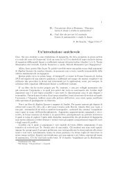
curves and generates self-intersecting surfaces like that in Figure 23.1, which
occur in the theory of Riemann surfaces [AhSa]. It all relates to the topological
picture of SO(3) as a closed “ball” in R 3 for which antipodal points of the
boundary are identified, as explained in Section 23.4.
Figure 23.1: A ruled surface generated by a rotation curve
Rotation curves, the subject of Section 23.5, are simply curves whose trace
lies in SO(3), rather than in R 3 . In practical terms, one can think of such a
curve as a “static fairground ride” in which the rider is strapped inside a sphere
which rotates about its center, with varying axis, and the parameter t is time.
One can also associate a rotation curve to a more dynamic rollercoaster-type
ride using the Frenet frame construction of Chapter 7. Section 23.7 briefly
discusses this and other topics. In the intervening Section 23.6, we explain how
Euler angles are used to decompose any rotation in space into the product of
rotations about coordinate axes.
There is a sense in which this chapter is a bridge between past and future
topics. The linear algebra reaches back to the start of the book, while Section
23.5 relates to homotopy and the theory of space curves in Chapters 6 and
7. On the other hand, the study of rotations and quaternions provides simple
examples of differentiable manifolds and related techniques that we shall meet
in the next chapter.

23.1. ORTHOGONAL MATRICES 769
23.1 Orthogonal Matrices
As explained at the outset in Section 1.1, one can represent a linear mapping
R n → R m by a matrix of size m × n. In this chapter, we shall be mainly
concerned with the case m = n = 3, but to begin with we impose only the
restriction m = n. This being the case, one can compose two linear mappings
A, B to make a third, denoted A ◦ B, defined by
(23.1)
(A ◦ B)(v) = A(B(v)), v ∈ R n .
If one regards A, B as matrices rather than mappings, then it is obvious from
(23.1) that their composition A ◦ B corresponds to the matrix product AB.
One only has to remember that it is actually B (or, more generally, the second
factor) that is applied first to a column vector in R n .
By its very definition, composition of mappings A, B, C : R n → R n satisfies
the associative law
(23.2)
A ◦ (B ◦ C) = (A ◦ B) ◦ C,
which forms part of the definition of a group (see page 131). The same is
of course true of matrix multiplication, and in Section 5.1 we defined various
groups by imposing restrictions on the linear transformations or matrices under
consideration. In this chapter, the emphasis will be on matrices, and we begin
with
Definition 23.1. An n × n matrix A is said to be orthogonal if
(23.3)
A T A = I n ,
where I n is the identity matrix of order n.
Recall that A T denotes the transpose of A, obtained by swapping its rows and
columns. Equation (23.3) therefore asserts that the columns of A form an
orthonormal basis of R n . For this reason, it would be more logical to speak of
an “orthonormal” matrix, though one never does.
Let O(n) denote the set of all orthogonal n × n matrices. Provided we
represent a linear transformation with respect to a fixed orthonormal basis,
O(n) coincides with the group orthogonal(R n ), via equation (5.2). The fact that
O(n) is a group can be seen directly by observing that if A, B ∈ O(n), then
(AB) T (AB) = B T A T AB = B T I n B = I n .
Moreover, the inverse of an orthogonal martrix is given by
A −1 = A T ,

770 CHAPTER 23. ROTATION USING QUATERNIONS
from which it follows that AA T = I n , or that the rows of A also form an
orthonormal basis.
Lemma 5.2 tells us that the determinant of any orthogonal matrix is either
1 or −1. Since det(AB) = (detA)(det B), it follows that the set
SO(n) = {A ∈ O(n) | detA = 1}
is a subgroup of O(n); that is, a group in its own right with the same operation of
matrix multiplication. The letter S stands for “special,” and SO(n) corresponds
to the group of orientation-preserving orthogonal transformations, or rotations,
as they were called on page 128.
We now specialize to the case n = 3 for which there is already a clear notion
of “rotation,” meaning a transformation leaving fixed the points on some straight
line axis, and rotating any other point in a plane perpendicular to the axis. An
example of such a rotation is the transformation represented by the matrix
⎛
⎞
(23.4)
R θ
=
⎜
⎝
cosθ − sin θ 0
sinθ cosθ 0
0 0 1
where 0 θ < 2π. This mapping leaves fixed the z-axis, but acts as a rotation
by an angle θ counterclockwise in the xy-plane.
The following well-known result implies that any element of SO(3) is equivalent
to some R θ
after a change of orthonormal basis.
Lemma 23.2. Given a 3 × 3 matrix A ∈ SO(3), there exists P ∈ SO(3) and
θ ∈ [0, 2π) such that
P −1 AP = R θ
.
Proof. The first step is to show that 1 is an eigenvalue of A. This is true
because
det(A − I 3 ) = det(A − AA T ) = det ( A(I 3 − A) T)
⎟
⎠ ,
= (detA)det ( (I 3 − A) T)
= − det(A − I 3 )
is zero. Since A − I 3 is singular, there exists a nonzero column vector w such
that Aw = w, and it is this eigenvector that determines the axis of rotation.
Extend the unit vector w 3 = w/‖w‖ to an orthonormal basis {w 1 ,w 2 ,w 3 } such
that w 1 × w 2 = w 3 . Being a positively oriented orthogonal transformation, A
must restrict to a rotation in the plane generated by w 1 ,w 2 , and there exists θ
such that ⎧
⎨ Aw 1 = w 1 cosθ + w 2 sinθ
(23.5)
⎩ Aw 2 = −w 1 sinθ + w 2 cosθ.

23.1. ORTHOGONAL MATRICES 771
Now let P denote the invertible matrix whose columns are the vectors w 1 ,w 2 ,w 3 .
By definition of matrix multiplication, the columns of AP are Aw 1 , Aw 2 , Aw 3 ,
and (23.5) now implies that AP = PR θ
. The result follows.
Lemma 23.2 can be expressed by saying that A is conjugate to R θ
in the
group SO(n). The two rotations are equivalent, if we are willing to change our
frame of reference by pointing the z-axis in the direction of the eigenvector w.
Combining (23.6) with equation (13.18) on page 398 gives
(23.6)
tr A = tr(PR θ
P −1 ) = tr(R θ
) = 2 cosθ + 1.
This means that the unsigned angle ±θ can conveniently be recovered from the
matrix A. To see how to recover the axis of rotation, see Exercise 4.
Later in this chapter, we shall be considering curves in the group SO(3).
Such a curve is a mapping γ: (a, b) → R 3,3 where (a, b) ⊆ R and R 3,3 is the
space of 3 × 3 matrices, and the problem is to find conditions that ensure that
the image of γ lies in SO(3). One method is to use a power series
(23.7)
γ(t) = I + A 1 t + A 2 t 2 + · · ·
where I = I 3 , and seek appropriate conditions on the coefficients. For example,
to determine A 1 , we need only consider the terms up to order one, and set
I = γ(t)γ(t) T = (I + A 1 t + · · ·)(I + A 1 t + · · ·) T
= I + (A 1 + A T 1 )t + · · ·
It follows that A 1 must be a skew-symmetric matrix, meaning A 1 T = −A 1 .
Having made the crucial step, it is in fact possible to solve (23.7) using the
concept of exponentiation. The exponential of a square matrix A, written e A or
exp A, is defined by the usual infinite sum
(23.8)
expA =
∞∑
k=0
1
k! Ak ,
with the convention that A 0 = I. This operation is well known to share some
of the usual properties of exponentiation of real numbers. In particular, (23.8)
converges, and if A, B are two square matrixes for which AB = BA then
exp(A + B) = (expA)(exp B).
If 0 denotes the zero matrix then obviously exp(0) = I. Thus,
exp(−A) = (expA) −1 ,
and the matrix (23.8) is always invertible.

772 CHAPTER 23. ROTATION USING QUATERNIONS
Any property valid for the powers of a matrix will extend to the operation of
exponentiation. For example, (A n ) T = (A T ) n for all n 0, and so exp(A T ) =
(exp A) T . A more interesting formula is
(23.9)
det(exp A) = exp(tr A).
This is immediate if A is diagonal with entries λ 1 , . . . , λ n , for then e A is diagonal
with entries e λ1 , . . .e λn , and (23.9) becomes the identity
n∏
e λi = e λ1+···+λn .
i=1
Having seen this, the validity of (23.9) can easily be extended to the case in
which A is diagonalizable (over the complex numbers). For then there exists
a complex invertible matrix P and a complex diagonal matrix D for which
A = PDP −1 , and
exp A = exp(PDP −1 ) =
=
∞∑
k=0
∞∑
k=0
1
k! (PDP −1 ) k
1
k! PDk P −1 = P(exp D)P −1
The result (23.9) now follows from the properties (13.18) already used for (23.6).
It is a general principle that, to prove a matrix equation like (23.9) (in
which both sides are continuous matrix functions), it suffices to assume that A is
diagonalizable. This is because an arbitrary square matrix can be approximated
by a sequence of diagonalizable matrices (for example, ones that have distinct
complex eigenvalues). In this way (23.9) follows in general; see [Warner] for a
fuller discussion of the exponentiation of matrices. The same principle can be
used to prove the Cayley–Hamilton Theorem (mentioned on page 402), namely
that any n × n matrix A satisfies its characteristic polynomial
c A (x) = det(xI n − A).
This theorem implies that the nth power A n is always some linear combination of
I n , A, A 2 , . . . , A n−1 . The same is therefore true of expA, and a vivid illustration
of this fact is provided by Theorem 23.4 below.
Lemma 23.3. If A is a n ×n skew-symmetric matrix, then exp A is an orthogonal
matrix with determinant 1.
Proof.
We have
exp(A T A) = exp(A T )exp A = exp(−A)exp A = (exp A) −1 exp A = I n .
Given that tr A = 0, the statement about det A = 1 follows from (13.18).

23.1. ORTHOGONAL MATRICES 773
The importance of this lemma can be assessed by the fact that it is related to
at least two topics studied in later chapters. 2
Any skew-symmetric 3×3 matrix is uniquely determined by a column vector
⎛ ⎞
x
⎜ ⎟
x = ⎝ y ⎠ ∈ R 3
z
by means of the formula
(23.10)
A[x] =
⎛
⎜
⎝
⎞
0 −z y
⎟
z 0 −x ⎠.
−y x 0
We need not have used coordinates, since (23.10) is equivalent to stating that
(23.11)
A[x]w = x × w
for all w ∈ R 3 . To understand this, consider
⎛ ⎞ ⎛ ⎞ ⎛ ⎞
1 0 0
⎜ ⎟ ⎜ ⎟ ⎜ ⎟
(23.12) e 1 = ⎝ 0⎠ , e 2 = ⎝ 1⎠ , e 3 = ⎝ 0⎠ ,
0 0 1
and observe that the ith row of A[x] is (the transpose of) the vector cross
product e i × x. Thus, the ith entry of the column vector A[x]w equals
(e i × x) · w = e i · (x × w),
explaining the appearance of the cross product of x with w.
The next result is a basic example for the mathematical theory of Lie groups
[DuKo], and is also well known in the context of computer vision [Faug].
Theorem 23.4.
(23.13)
(i) Let x be a nonzero vector in R 3 and set l = ‖x‖. Then
exp A[x] = I + sin l 1 − cosl
A[x] +
l l 2 A[x] 2 .
(ii) any nonidentity P ∈ SO(3) can be written in this form; indeed (23.13)
represents a rotation with axis parallel to x and angle l.
We choose to postpone the proof of (ii), which demonstrates the simplicity with
which rotations can be represented via linear algebra. It is accomplished by
Corollary 23.14.
2 The set of skew-symmetric n × n matrices forms what is called a Lie algebra when one
defines [A, B] = AB − BA (see Exercise 5 and page 832). There exists a means of exponentiating
any finite-dimensional Lie algebra to obtain a Lie group, thus generalizing Lemma 23.3
[Warner]. There is a more general notion of exponentiation in Riemannian geometry, whereby
the tangent space of a surface acts to model the surface itself (see page 885).

774 CHAPTER 23. ROTATION USING QUATERNIONS
Proof of (i). Let l = ‖x‖, and set x 1 = x/l. Choose a unit vector x 2 orthogonal
to x and let x 3 = x 1 × x 2 . With respect to the basis {x 1 ,x 2 ,x 3 }, the linear
transformation (23.11) associated to A[x] has matrix
⎛ ⎞
(23.14)
⎜
⎝
0 0 0
0 0 −l
0 l 0
There is a similarity with (23.4), explained by the fact that (23.14) equals A[le 1 ],
and A[x] acts as l times the operator J in the plane generated by x 2 and x 3 .
Both A[le 1 ] and A[x] have eigenvalues 0, il, −il. Indeed, A[le 1 ] = PDP −1
where ⎛ ⎞ ⎛ ⎞
P =
⎜
⎝
1 0 0
0 i 1
0 1 i
The matrix D satisfies the equation
⎟
⎠, D =
⎟
⎠.
⎜
⎝
0 0 0
0 il 0
0 0 −il
e x = 1 + sin l
l x + 1 − cosl
l 2 x 2
(with D in place of x and I 3 in place of the first 1) because each of its diagonal
entries does. The same equation is satisfied by A[x] because
exp(PDP −1 ) = P(exp D)P −1
⎟
⎠ .
= I 3 + sinl
l PDP −1 + 1 − cosl
l 2 (PDP −1 ) 2 .
1
0.8
0.6
0.4
0.2
0.5 1 1.5 2 2.5 3
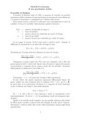
Figure 23.2: The functions sin l
l
and 1 − cosl
l 2
Figure 23.2 plots the functions occurring in (23.13) over the range 0 l π
that will interest us in Section 23.4. Both tend to a limit as l → 0, so we may
allow x = 0 in (23.13), as this is consistent with the formula exp0 = I.

23.2. QUATERNION ALGEBRA 775
We shall return to the theory underlying Theorem 23.4 after the introduction
of quaternions.
23.2 Quaternion Algebra
At one level, a quaternion is merely a vector with four components — that is an
element of 4-space — and we explore this aspect first. By analogy to complex
numbers, one denotes an individual quaternion by
(23.15)
q = a + bi + cj + dk, a, b, c, d ∈ R,
and the set of quaternions by H. Since q is determined by the vector (a, b, c, d),
the set H can be identified with R 4 as a vector space. But the real beauty of H
derives from the special way in which its elements can be multiplied.
The multiplication of quaternions is based on the “fundamental formula”
i 2 = j 2 = k 2 = ijk = −1,
that Hamilton 3 carved into Brougham bridge in 1843. It satisfies the associative
rule (analogous to (23.2) without the ◦ ), which asserts that there is no ambiguity
in computing a product of three or more quaternions written in a fixed
order (this is Corollary 23.6 overleaf). For example,
−i = j 2 i = jji = j(ji) = j(−k) = −jk.
Indeed, it is frequently convenient to regard i,j,k as equal to the respective
vectors e 1 ,e 2 ,e 3 in (23.12). Their multiplication is then derived from the vector
cross product in R 3 .
Now that we have defined quaternion multiplication, one can appreciate that
the four coordinates a, b, c, d on the right-hand side of (23.15) are not equivalent.
Indeed, R 4 is split up into R and R 3 , and we can distinguish the real part
and the imaginary part
Req = a,
Imq = bi + cj + dk
of any quaternion. Unlike for complex numbers (in which the imaginary part of
z = x + iy is the real number y), the imaginary part of q is effectively a vector
in R 3 . One says that q is an imaginary quaternion if Req = 0.
We shall often write
(23.16)
q = a + v,
with the understanding that v = Imq ∈ R 3 .
3 See page 191.

776 CHAPTER 23. ROTATION USING QUATERNIONS
Lemma 23.5. If q 1 = a 1 + v 1 and q 2 = a 2 + v 2 , then
(23.17)
Re(q 1 q 2 ) = a 1 a 2 − v 1 · v 2 ,
Im(q 1 q 2 ) = a 1 v 2 + a 2 v 1 + v 1 × v 2 .
In particular, if q 1 = v 1 and q 2 = v 2 are imaginary quaternions, then
(23.18)
Proof.
q 1 q 2 = −v 1 · v 2 + v 1 × v 2 .
This is just a matter of expanding brackets:
q 1 q 2 = (a 1 + v 1 )(a 2 + v 2 )
= (a 1 a 2 − v 1 · v 2 ) + (a 1 v 2 + a 2 v 1 + v 1 × v 2 ).
The last statement follows from setting a 1 = 0 = a 2 .
The next result is verified in Notebook 23.
Corollary 23.6. Multiplication of quaternions is associative:
for all q 1 ,q 2 ,q 3 ∈ H.
(q 1 q 2 )q 3 = q 1 (q 2 q 3 ),
Of course, quaternion multiplication is not commutative, by its very definition
(but see Exercise 2).
The following will help us emphasize similarities between H and C.
Definition 23.7. Let q = a + bi + cj + dk = a + v ∈ H.
(i) The modulus or norm of q, written |q|, is given by
|q| 2 = a 2 + b 2 + c 2 + d 2 = a 2 + ‖v‖ 2 .
Moreover, q is called a unit quaternion if |q| = 1.
(ii) The conjugate of q, written q, is given by
q = a − bi − cj − dk = a − v.
Thus, the norm of q is simply its norm as a vector in R 4 , as defined on page 3.
Because of the analogy with complex numbers (and anticipating Lemma 23.8),
we indicate the norm with a single vertical line, rather than two. For consistency,
we shall also indicate the norm of a vector v ∈ R 3 by |v|, rather than ‖v‖,
because in this chapter we shall usually be thinking of such a vector as the
imaginary quaternion q = 0 + v.

23.2. QUATERNION ALGEBRA 777
The conjugate of a quaternion q is formed by reversing the sign of its imaginary
component. We shall use the expression Im H to indicate the space
{q ∈ H | q = −q}
of imaginary quaternions. It is effectively R 3 , but using the definitions above, we
can multiply two elements of Im H according to the rule (23.18). In particular,
if q = v is an imaginary quaternion, then
(23.19)
q 2 = v 2 = −v · v = −|v| 2
is a real number.
The key properties underlying Definition 23.7 are encapsulated in
Lemma 23.8. Let q,q 1 ,q 2 ∈ H. Then
(i) qq = |q| 2 ;
(ii) q 1 q 2 = q 2 q 1 ;
(iii) |q 1 q 2 | = |q 1 ||q 2 |.
Proof. Part (i) follows from (23.19), given that (a + v)(a − v) = a 2 − v 2 .
Part (ii) is an immediate consequence of equation (23.17), and the fact that
−v 1 × v 2 = v 2 × v 1 . Given (i),
|q 1 q 2 | 2 = q 1 q 2 q 1 q 2
= q 1 q 2 q 2 q 1 = q 1 |q 2 | 2 q 1 = |q 1 | 2 |q 2 | 2 .
Part (i) of this lemma has an important consequence. It exhibits explicitly the
inverse of a nonzero quaternion, namely
q −1 = 1 q, q ≠ 0.
|q|
This means that H is a division ring or skew­field, an algebraic structure with
all the properties of a field except commutativity [Her, CoSm].
At this point, the multiplication rules allow one to regard a complex number
as a quaternion for which c = d = 0. However, this is to miss the point, since
we could have equally well chosen j or k to play the role of the symbol i = √ −1
used to define complex numbers. Indeed, if v ∈ Im H is any fixed unit imaginary
quaternion, we can identify the real 2-dimensional subspace
(23.20)
〈 1, v 〉 = {a + bv | a, b ∈ R}
with C by means of the mapping
a + ib ↦→ a + bv.

778 CHAPTER 23. ROTATION USING QUATERNIONS
The multiplications (of C on the one hand and Im H on the other) are consistent,
because
(a 1 + b 1 v)(a 2 + b 2 v) = a 1 a 2 + (a 1 b 2 + b 1 a 2 )v + b 1 b 2 v 2
= (a 1 a 2 − b 1 b 2 ) + (a 1 b 2 + b 1 a 2 )v.
The set of unit imaginary quaternions is parametrized by the unit sphere S 2 (1);
in conclusion, there is a whole sphere’s worth of complex planes incorporated
into H! This multiple way in which H extends C is what is understood by the
term “hypercomplex geometry” when applied in relation to the quaternions.
Writing out Lemma 23.8(iii) (squared) in full gives the identity
(23.21)
(a 1 2 + b 1 2 + c 1 2 + d 1 2 )(a 2 2 + b 2 2 + c 2 2 + d 2 2 ) = a 3 2 + b 3 2 + c 3 2 + d 3 2 ,
where (copying from Notebook 23),
a 3 = a 1 a 2 − b 1 b 2 − c 1 c 2 − d 1 d 2 ,
b 3 = a 2 b 1 + a 1 b 2 − c 2 d 1 + c 1 d 2 ,
c 3 = a 2 c 1 + a 1 c 2 + b 2 d 1 − b 1 d 2 ,
d 3 = −b 2 c 1 + b 1 c 2 + a 2 d 1 + a 1 d 2 .
Now consider what happens when the components of q 1 and q 2 are all integers.
We see that the product of two sums of four squared integers is itself a sum of
four squared integers. This fact is the crucial first step in proving the following
result of Lagrange.
Theorem 23.9. Any positive integer n can be written as the sum
(23.22)
n = a 2 + b 2 + c 2 + d 2 ,
a, b, c, d ∈ N
of four squares of nonnegative integers.
In the light of (23.21), it is sufficient to prove the result when n is a prime
number, and we refer the reader to any standard text on elementary number
theory, such as [Baker].
The representation (23.22) is in general far from unique. For example, it
is verified in Notebook 23 that if n = 100 then the solutions (a, b, c, d) with
a b c d are
(5, 5, 5, 5), (7, 5, 5, 1), (7, 7, 1, 1), (8, 4, 4, 2), (8, 6, 0, 0), (9, 3, 3, 1), (10, 0, 0, 0).
Three of them are implicit in the quaternionic factorization
(1 + i + j + k)(3 − 4j) = 7 + 7i − j − k.

23.3. UNIT QUATERNIONS 779
23.3 Unit Quaternions and Rotations
We have seen (Corollary 23.6) that quaternions obey the associative rule. The
set H is not itself a group because the quaternion 0 has no multiplicative inverse,
though the set H \ {0} is a group under multiplication. So is the set
U = {q ∈ H | |q| = 1}
of unit quaternions. This follows from Lemma 23.8 since if q 1 ,q 2 ∈ U then
|q 1 q 2 | = |q 1 ||q 2 | = 1,
and U is closed under products. Also, if q ∈ U then
q −1 = q ∈ U ,
showing that U is closed under taking inverses, and the rules on page 131 are
satisfied. Readers who are not familiar with U may nonetheless be acquainted
with its finite subgroup Q 8 of eight elements (see Exercise 3).
Since a unit quaternion has the form
q = a + bi + cj + dk, with a 2 + b 2 + c 2 + d 2 = 1,
U can be identified with the set
{
(a, b, c, d) ∈ R 4 : a 2 + b 2 + c 2 + d 2 = 1 } .
(23.23)
This is none other than the hypersphere S 3 (1), consisting of all the 4-vectors a
unit distance from the origin (see similar definitions on pages 236 and 662).
The aim of this section is to show that U is intimately related to the group
SO(3) of rotations in R 3 . The starting point is
Lemma 23.10. Let q ∈ U . If w ∈ Im H then qwq is an imaginary quaternion
with the same norm as w. The resulting mapping
(23.24)
is an orthogonal transformation of R 3 .
w ↦→ qwq
Proof. By hypothesis, w = −w and w 2 = −|w| 2 . Let p = qwq. The property
of conjugation implies that
p = q w q = q(−w)q = −p.
It follows that p is also an imaginary quaternion; we compute
(23.25)
|p| 2 = pp = (qwq)(−qwq)
= q(−w 2 )q
= q|w| 2 q = |w| 2 .
The mapping w ↦→ p is certainly linear, and the last statement now follows
from the proof of Theorem 5.6 on page 132.

780 CHAPTER 23. ROTATION USING QUATERNIONS
We denote the transformation (23.24) by R[q]. Thus, if q = a + v ∈ U ,
then
R[q]w = (a + v)w(a − v)
(23.26)
= a 2 w + a(vw − wv) − vwv, w ∈ Im H.
The consequences of this calculation are pursued in the following key result in
the subject.
Theorem 23.11. Let q be a unit quaternion. Then R[q] represents a counterclockwise
rotation by the angle 2 arccos(Req), measured between 0 and 2π, with
axis pointing in the direction of Imq.
The qualification counterclockwise is to be interpreted when one looks downwards
from a “mast” pointing in the direction of Imq onto the perpendicular
plane of rotation. This is equivalent to the “right-hand corkscrew rule.”
Proof. Write v = Imq and q = a +v ∈ U . There is a unique number θ, with
0 θ 2π such that a = cos(θ/2), and so |v| = sin(θ/2) 0.
If v = 0 then q = ±1 and θ is 0 or 2π, which gives rise to the identity rotation,
and accords with the statement of the theorem. Hence, we may assume that
|v| ≠ 0. Observe too that equation (23.26) implies that
(23.27)
R[q]v = a 2 v + |v| 2 v = v.
Next, choose a unit imaginary quaternion w 1 perpendicular to v in Im H = R 3 .
Then w 1 · v = 0 and vw 1 = −w 1 v = v × w 1 . If we set
w 3 = 1
|v| v, w 2 = w 3 w 1 ,
then {w 1 ,w 2 ,w 3 } is an orthonormal basis of R 3 with w 1 ×w 2 = w 3 . Moreover,
using (23.26),
(23.28)
Similarly,
(23.29)
R[q]w 1 = w 1 cos 2 θ
2 + 2vw 1 cos θ 2 − w 1 sin 2 θ
2
= w 1 cosθ + w 2 sin θ.
R[q]w 2 = w 2 cos 2 θ
2 + 2vw 2 cos θ 2 − w 2 sin 2 θ
2
= w 2 cosθ − w 1 sin θ,
exactly as in (23.5). Equations (23.27), (23.28), (23.29) assert that the linear
transformation R[q] has matrix (23.4) relative to the orthonormal basis
{w 1 ,w 2 ,w 3 }, and is the rotation stated in the theorem.

23.3. UNIT QUATERNIONS 781
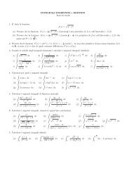
Note that both q and −q determine the same transformation; this is related
to the appearance of half-angles θ/2. Computationally, it is now an easy matter
to use quaternions to model rotations, such as the one that Figure 23.3 attempts
to represent:
Figure 23.3: A rotation of the sine surface by R[ 1 √
2
+ 1 2 j + 1 2 k]
The mapping
(23.30)
U −→ SO(3)
q ↦→ R[q]
satisfies the important property
(23.31)
R[q 1 q 2 ] = R[q 1 ] ◦ R[q 2 ].
This follows from its definition (23.24), since R[q 1 q 2 ] is the transformation
w ↦→ (q 1 q 2 )w(q 1 q 2 ) = q 1 (q 2 wq 2 )q 1 .
Equation (23.31) characterizes what is called a group homomorphism, a mapping
from one group to another that preserves the respective multiplication rules.
(For this topic, we recommend [Her, chapter 2].)
At this stage, we choose to write R[q] explicitly as a 3×3 orthogonal matrix.
Referring to Lemma 23.2, this matrix is obtained by conjugating (23.4) by the
orthogonal matrix whose columns are the orthonormal triple w 1 ,w 2 ,w 3 . The
result is well known and is computed in Notebook 23:

782 CHAPTER 23. ROTATION USING QUATERNIONS
Proposition 23.12. Let q = (a, b, c, d) be a unit quaternion. Then the rotation
R[q] has matrix
⎛
⎞
a 2 + b 2 − c 2 − d 2 2bc − 2ad 2ac + 2bd
⎜
⎝ 2bc + 2ad a 2 − b 2 + c 2 − d 2 ⎟
(23.32)
2cd − 2ab ⎠ .
2bd − 2ac 2ab + 2cd a 2 − b 2 − c 2 + d 2
In Notebook 23, we also verify directly that this matrix has determinant 1, even
though this fact is a consequence of the proof of Theorem 23.11. It also follows
from (23.26) and a continuity argument, as detR[q] cannot jump from 1 to −1.
It is tempting to say that (23.32) is completely determined by the imaginary
part Imq = (b, c, d) by defining
a = √ 1 − b 2 − c 2 − d 2 .
This is not quite true, because Req may be negative, and changing the overall
sign of q to adjust for this has the effect of reversing the sign of v and the angle
of rotation. Nevertheless, there is a very natural way of converting a 3-vector
into a rotation, and we describe this in the next section.
As an application of Theorem 23.11, consider the composition of two rotations
R[q 1 ], R[q 2 ] about axes v 1 ,v 2 with respective angles θ 1 , θ 2 . The combined
rotation (23.31) is easiest to identify in the case in which the vectors v 1 and v 2
are orthogonal:
Corollary 23.13. If v 1 · v 2 = 0, the composition R[q 1 q 2 ] is a rotation through
an angle θ with
and parallel to the axis
cos θ 2 = cosθ1 2 cosθ2 2 ,
sin θ1
2 cosθ2 2 i + cosθ1 2 sinθ2 2 j + sinθ1 2 sinθ2 2 k.
Proof. Without loss of generality, we may assume that v 1 ,v 2 are parallel to
the coordinate axes x, y. Then
q 1 = a 1 + b 1 i, q 2 = a 2 + b 2 j,
where a i = cos(θ i /2) and b i = sin(θ i /2). Thus,
q 1 q 2 = a 1 a 2 + b 1 a 2 i + a 1 b 2 j + b 1 b 2 k,
and we can obtain the required formulas, bearing in mind that q 1 q 2 is again a
unit quaternion.

23.4. IMAGINARY QUATERNIONS 783
23.4 Imaginary Quaternions and Rotations
The secret of using vectors to achieve rotations relies on the following fact,
which (only) at first sight appears to have nothing to do with quaternions. Any
rotation can be represented by a vector x in R 3 with |x| π, by means of the
following rule:
the axis of rotation is in the direction given by x, and the angle of
rotation is |x| radians counterclockwise.
The representation above is almost unique, but there is an inevitable ambiguity,
this time only if |x| = π. (Recall that, in this chapter, |x| denotes the usual
Euclidean norm ‖x‖.) For in this case, both x and −x represent the same
rotation by π radians or 180 o . This is because a rotation of θ counterclockwise
about x is the same thing as a rotation of −θ or 2π − θ counterclockwise about
−x, and the two coincide if θ = π.
The description above incorporates a significant fact. To explain it, we first
define the closed ball
(23.33)
B 3 (π) = {x ∈ R 3 | |x| π},
consisting of the sphere S 2 (π) of radius π, together with all its interior points.
We are therefore saying that the set SO(3) of rotations can be thought of as the
set B 3 (π) in which antipodal points on the boundary sphere S 2 (π) are identified.
For if |x| = π, then x and −x are different points in B 3 (π) that define the same
rotation. The idea is that a bookworm living inside the ball that tunnels to the
boundary does not get outside the sphere, but re-emerges at the point inside
diametrically opposite the point it left.
It is a consequence of the description above that the set SO(3) of rotations
forms a topological space without boundary. Mathematically, the sort of operation
that has been performed on B 3 (π) to obtain SO(3) is a higher-dimensional
analogue of the type of identifications carried out in Section 11.2. The argument
after Figure 11.16 on page 346 shows that the disk B 2 (π) in R 2 with points of its
boundary circle S 1 (1) identified gives rise to the cross cap surface. The latter is
a realization of the real projective plane RP 2 , which parametrizes straight lines
passing through the origin in R 3 . The same argument can be repeated to see
that the set SO(3) is topologically the real projective 3-space RP 3 parametrizing
lines through the origin in R 4 ; see Exercise 12.
To understand the link with quaternions, we need to represent analytically
the rotation defined by the vector x. We can do this quickly using the machinery
of the previous section. Let l = |x| denote the required angle of rotation, this
time with 0 < l π. Set
a = cos l (
2 0, v = sin
2) l x (23.34)
l .

784 CHAPTER 23. ROTATION USING QUATERNIONS
Then q = a+v is a unit quaternion, whose imaginary part v has norm sin(l/2).
Theorem 23.11 implies that R[q] is the required rotation. Recalling the notation
(23.10), we can use this to establish
Corollary 23.14. Let x ∈ B 3 (π). The matrix of the rotation R[q] (with axis x
and counterclockwise angle |x|) equals exp A[x].
This result is effectively Theorem 23.4(ii), whose proof we now give.
Proof.
Having fixed x, we use (23.34), and temporarily abbreviate
A = A[v] = sin(l/2) A[x].
l
Bearing in mind the form of equation (23.13), we shall express A 2 using quaternion
multiplication. Assume first that w is perpendicular to v. Then
2A 2 w = 2A(v × w) = v × (2v × w)
(23.35)
= v × (vw − wv)
= 1 (
)
v(vw − wv) − (vw − wv)v
2
= −vwv − |v| 2 w.
Since vw − wv = 2vw and a 2 + |v| 2 = 1, we may re-write (23.26) as
R[q]w = w + 2aAw + 2A 2 w.
This relation also holds when w is parallel to v because of (23.27). In conclusion,
as expected.
R[q] = I 3 + 2 cos l 2 A + 2A2
= I 3 + sinl A[x] + 1 − cosl
l l 2 A[x] 2 ,
It follows that
SO(3) = {expA[x] | |x| π},
so that the composition exp ◦A maps the closed ball B 3 (π) onto SO(3).
The descriptions we have seen make it easy to model rotations, a careful
choice of which can be used to view the details of a surface. Figure 23.4 is a
single frame of an animation from Notebook 23 of a truncated view of the sine
surface, designed to reveal its inners (the axis of rotation is visible). Lines of
self-intersections meet in a more complicated singularity at the origin.

23.5. ROTATION CURVES 785
Figure 23.4: Viewing singularities of the sine surface
23.5 Rotation Curves
The theory of the preceding section taught us to associate to any vector x
in the ball B 3 (π) a rotation in space, and to represent this rotation by the
orthogonal matrix expA[x]. In practice, this is best calculated using the formula
of Theorem 23.4, which we now know arises from the unit quaternion
(23.36)
q = cos(l/2) + sin(l/2) x, l = |x| π,
l
defined by (23.34). The only ambiguity occurs when |x| = π for then ±x give
rise to the same unit quaternion q.
Let c j denote the j th column of the matrix (23.32) representing (23.36). It
is the image of the j th basis element (from the list (23.12)) under the rotation.
Since a 2 + b 2 + c 2 + d 2 = 1, we have
⎛
⎞ ⎛ ⎞
−2c 2 − 2d 2 + 1 1
⎜
⎟ ⎜ ⎟
c 1 = ⎝ 2bc + 2ad ⎠ = R[q] ⎝ 0⎠ .
2bd − 2ac 0
The fact that R[q] is a rotation translates into the identity
(23.37)
c 1 × c 2 = c 3 .

786 CHAPTER 23. ROTATION USING QUATERNIONS
In particular, it means that R[q] is completely determined by the first two
columns c 1 ,c 2 .
We can now work backwards, and attempt to construct (23.32), R[q] and
ultimately x itself from the columns of (23.32). If we start from the first column,
the only restriction is that it be a unit vector, so
c 1 ∈ S 2 (1).
However, having fixed c 1 , the next column c 2 must be chosen perpendicular to
c 1 . This having been done, c 3 is completely determined by (23.37).
Let M = S 2 (1). If u ∈ M, then the orthogonal complement
u ⊥ = {w ∈ R 3 | u · w = 0}
can be identified with the tangent space M u . In general, the set
{(u,w) | u ∈ M, w ∈ M u }
is called the tangent bundle of the surface M, and is discussed in a more general
setting in the next chapter (within Section 24.5). But for the moment, it leads
to yet another description of the set SO(3).
Proposition 23.15. The set SO(3) is in bijective correspondence with the unit
tangent bundle
{(u,w) | u,w ∈ S 2 (1), u · w = 0}
of the unit sphere.
Note the symmetry between u and w in this definition.
Proposition 23.15 is relevant to the next topic. At the start of this book,
on page 5, we defined a curve in R n , and in Chapters 7 we specialized to the
case n = 3. We are now in a position to adapt this to the case in which R 3 is
replaced by SO(3).
Definition 23.16. A rotation curve is a mapping γ : [a, b] → SO(3) of the form
γ(t) = exp A[α(t)],
where α: [a, b] → R 3 is a parametrized curve whose image lies in B 3 (π). The
rotation curve is closed if γ(a) = γ(b).
We begin with two basic examples of such curves.
(i) Fix a unit vector u, and set
α(t) = tu, −π t π.
Then γ(t) = exp A[tu] is a rotation, by an angle t, about a fixed axis
parallel to u. The curve α is a diameter of B 3 (π), but γ is closed since
expA[−πu] = expA[πu].

23.5. ROTATION CURVES 787
(ii) Fix an orthonormal pair u 1 ,u 2 of vectors, and set
β(t) =
(
u 1 cos t 2 + u 2 sin t )
π, −π t π.
2
The trace of β is half of a great circle lying on the boundary S 2 (π) of
B 3 (π), and every element δ(t) = expA[β(t)] is a rotation of 180 o . The
rotation curve δ is again closed since β(π) = πu 2 = −β(−π).
These two examples are almost identical, though this fact is partially hidden
by our preference for imaginary quaternions; matters become clearer when we
revert to unit quaternions. In case (i), the associated unit quaternion is
(23.38)
q(t) = cos t 2 + u sin t 2 ,
whereas for (ii), β(t) is itself a unit imaginary quaternion. Indeed, β(t) has the
same form as (23.38) with u 1 ,u 2 in place of 1,u; if we choose u = u 1 u 2 , then
β(t) = u 1 q(θ).
This means that
δ(t) = R[u 1 ]γ(t),
and the two rotation curves differ by the fixed 180 o rotation R[u 1 ]. In technical
language, left translation within the group U converts a diameter of B 3 (π) into
half a great circle.
Surprisingly complicated examples can be obtained by starting from a curve
whose trace lies in the intersection of B 3 (π) with a plane through the origin.
Using standard coordinates in R 3 , consider the ellipse
(23.39)
α[a, b](t) = ( 0, a cost, b sint ) π, −π t π,
where a, b are fixed positive numbers such that a 2 cos 2 t + b 2 sin 2 t 1 for all t.
Let γ(t) = exp A[α[a, b](t)]; both α[a, b] and γ are closed curves. To describe
γ, it suffices to specify the first two columns γ(t)e 1 and γ(t)e 2 in accordance
with the discussion leading to Proposition 23.15. As t varies, these generate two
curves lying on S 2 (π).
This example is animated in Notebook 23 and illustrated in Figure 23.5. One
can imagine a rigid body with two perpendicular arms that are constrained to
follow the respective spherical curves. In the frame shown, the rotation is about
to pass through a “vertex” in which one column achieves an extreme value, and
the second passes through the chicane in the figure eight.

788 CHAPTER 23. ROTATION USING QUATERNIONS
Figure 23.5: A rotation curve specified by its columns
Figure 23.6 concerns the case of (23.39) in which a = b and
γ[a](t) = exp(A[α[a, a]]), 0 t 2π.
From example (ii) above, γ[1] represents a rotation curve corresponding to
revolving two turns (4π radians or 720 o ) around a fixed axis. At the other
extreme, γ[0] is the “identity curve,” whose trace consists of the single point
I 3 ∈ SO(3). Figure 23.6 displays the intermediate curves γ[1−a] with a = n/17
and 1 n 16. In the first frame, the straightforward 720 o rotation has been
deformed slightly to γ[16/17] so that the axis begins to “wobble.” By the time
we get down to γ[4/17], represented by the first frame in the last row, a rigid
body subject to this family of rotations will merely rock slowly about an axis
lullaby-fashion (imagine Figure 23.5 with the more tranquil background).
The family
a ↦→ γ[1 − a], 0 a 1
is a continuous deformation from the “two turns curve” γ[1] to the identity
γ[0]. In the language of Section 6.3, it is a homotopy between γ[1] and γ[0].
There are other ways of demonstrating the existence of such a homotopy, such
as the so-called Dirac scissors trick (see [Pen, §11.3]). There exists no such
homotopy if we begin with the closed rotation curve γ[1] defined for 0 t π,
which corresponds to a single revolution. This fact is expressed by saying that
the topological space SO(3), which we have mentioned is equivalent to RP 3 ,
is not simply­connected — there exist closed curves that cannot be deformed

23.6. EULER ANGLES 789
to a point. It is however the case that the “double” of any closed curve can
always be deformed to a point. These facts are explained in introductory texts
to algebraic topology, such as [Arm].
Figure 23.6: A homotopy of rotation curves γ[ n 17 ]
23.6 Euler Angles
The traditional way to specify a rotation is to break it up into the composition
of three rotations about the three Cartesian axes. In practice, this is the method
used in fairground machinery, or in a gyroscope to align a navigation system.
In order to provide a vivid explanation of Euler angles, we define them
in relation to an aircraft taking off from runway 27L at Heathrow airport in
London, on its way to Paris. Imagine first a Cartesian frame of reference F 0
fixed in the center of the runway, with the x-axis due east, y-axis due north

790 CHAPTER 23. ROTATION USING QUATERNIONS
(which just happens to be perpendicular to the runway), and z (for “zenith”)
vertically upwards. As the aircraft passes by on its take-off run, its own frame
of reference F 1 (with x pointing to the nose and y to the port or left wing) is
obtained from F 0 by means of a rotation of 180 o about the z-axis, to give the
correct heading of 270 o . After takeoff, the aircraft climbs at a constant angle or
elevation of 20 o ; mathematically this is achieved by rotating F 1 by −20 o about
its y-axis, and produces a new frame of reference F 2 . At a height of 2000 feet,
the aircraft banks left, by rolling −30 o about its nose-tail or x-axis, temporarily
achieving the frame of reference F 3 .
z
x
Θ
Φ
Ψ
y
Figure 23.7: A sequence of rotations about axes z y x
To sum up, F 3 has been obtained from F 0 by means of a sequence of rotations
through
(23.40) ψ = 180 o , θ = −20 o , φ = −30 o
about the z-, y-, x-axes respectively (our notation is similar to that of [Kuipers,
4.4]). The triple (ψ, θ φ) comprises the Euler angles of the single rotation P
needed to move F 0 to F 3 , and can be regarded as yet another way of representing
a rotation by a 3-vector (albeit one whose three components are angles).

23.6. EULER ANGLES 791
To be more precise, we can interpret each frame F i as the orthonormal triple
of vectors defining the frame’s axes, and translate all the frames to a common
origin. In this way, F 3 is obtained from F 0 by the composition
of rotations, where
R[a 3 + b 3 i] ◦ R[a 2 + b 2 j] ◦ R[a 1 + b 1 k]
a 3 = cos φ 2 , a 2 = cos θ 2 , a 1 = cos ψ 2 .
One can easily compute P using Corollary 23.13.
The definition of the Euler angles depends on the sequence of axes chosen to
perform the respective three rotations. The above choice z y x (meaning
first z then y then x) is illustrated in Figure 23.7 but with a different choice of
angles (ψ = −2π/3, θ = −π/3, φ = +π/4 in radians). At each step the new
axes are shortened to help identify them, but the figure is best seen on screen
in color. One can attempt to use any other sequence to obtain a given rotation,
such as x y x, though it is useless if the same axis appears next to itself in
the sequence. It follows that there is a total of 3 ·2·2 = 12 choices for the triple,
but essentially only two types: those in which the three axes are different and
those in which the first and third coincide. As it happens, the standard rotation
package within Mathematica uses the sequence z x z (see Notebook 23).
Euler’s theorem states that any element in SO(3) can be decomposed as
the composition of three rotations about mutually orthogonal axes, in either
of the above ways we care to choose. Using the theory from Section 23.3, it
amounts to the following factorization result for unit quaternions. First, recall
the notation (23.20), and consider the circle
(23.41)
U v = {a + bv | a 2 + b 2 = 1}
formed by intersecting the subspace 〈 1, v 〉 with U .
Theorem 23.17. Let q ∈ U . Then there exist
(i) q 1 ∈ U i , q 2 ∈ U j , q 3 ∈ U k such that q = q 3 q 2 q 1 ;
(ii) p 1 ∈ U i , p 2 ∈ U j , p 3 ∈ U i such that q = p 3 p 2 p 1 .
We omit the proof, referring the reader to [Kuipers, chapter 8]. A first step
consists in the characterization of those quaternions that can be represented in
the form q 1 q 2 where q 1 ∈ U i and q 2 ∈ U j (see Exercise 8). To explain the
nature of the problem, we prove instead the following simpler result.
Lemma 23.18. Given v ∈ Im H, there exist a, b, c ∈ R such that
Im[(a + i)(b + j)(c + k)] = v.

792 CHAPTER 23. ROTATION USING QUATERNIONS
Proof.
(23.42)
Writing v = ri + sj + tk and expanding, we need to solve the system
⎧
⎪⎨ a + bc = r,
−b + ac = s,
⎪⎩
c + ab = t,
that does not quite have cyclic symmetry. Eliminating b, we obtain
{
a(1 + c 2 ) = cs + r,
Eliminating c gives the quintic equation
c(1 + a 2 ) = as + t.
a 5 − ra 4 + 2a 3 + (st − 2r)a 2 + (t 2 − s 2 + 1)a − r − st = 0,
which has at least one real root a. The last two equations in (23.42) are then
linear and can be solved for b and c.
There are well-documented disadvantages of the use of Euler angles to describe
rotations. Not only do they depend very much on the choice of axis
sequence, but are subject to an analog of gimbal lock of an inertial guidance
system. Fear of gimbal lock was the bane of mission control during the Apollo
moon landing and other space flights. One manifestation of the difficulty is
that when an Euler angle approaches π/2, its cosine approaches 0, and it is
impossible for a computer to perform division by cosθ. Mechanically, one can
partly understand the problem by supposing that our aircraft is able (quickly
after takeoff) to climb vertically, so that θ has become −90 o in (23.40). In these
circumstances, the aircraft’s heading has been “lost,” the third rotation could
have been achieved by changing the direction of the runway, and ψ, φ are no
longer independent parameters.
The advantage of our earlier description of rotations based on imaginary
quaternions is that the mapping B 3 (π) → SO(3) defined by
ρ(x) = exp A[x] = R[q]
is regular in the sense that the partial derivatives ρ x , ρ y , ρ z are always linearly
independent (as 3×3 matrices, or elements of R 9 ), in the spirit of Definition 19.16
on page 606. This is not true of the mapping σ: R → SO(3) defined by
σ(ψ, θ, φ) = F 3 ,
where R = [0, 2π] × [−π/2, π/2] × [−π, π] is the usual domain of definition for
the Euler angles. Indeed, we verify in Notebook 23 that the set
{
σ
(ψ, π ) ∣ } ∣∣
2 , φ ψ, φ ∈ R
is a curve and not a surface in SO(3).

23.7. FURTHER TOPICS 793
23.7 Further Topics
We conclude this chapter with some more applications. The first two link to
the themes of Chapters 7 and 15 respectively.
Frenet Frames Revisited
We can associate to each point of a space curve α: (a, b) → R 3 a rotation matrix
F(t) as follows. The parameter t need not be arc length. The columns of F(t)
are the unit tangent, normal and binormal vectors T(t),N(t),B(t) at the point
α(t). These are mutually orthogonal and by definition,
B(t) = T(t) × N(t).
It follows that F(t) lies in SO(3), and represents the rotation necessary to
transform the standard frame of reference {e 1 ,e 2 ,e 3 } to F(t), in analogy to the
aeronautical example of the previous section.
The assignment of the unit tangent vector T(t), thought of as a point on
S 2 (1), to α(t) is a type of Gauss map for the curve, although it could be argued
that using N(t) in place of T(t) is closer to the Gauss definition for surfaces.
The fact is that we may as well associate the whole Frenet frame F(t) to a point
α(t) where κ(t) ≠ 0. The resulting assignment
(23.43)
t ↦→ α(t) ↦→ F(t),
ultimately mapping the trace of α to SO(3), is an example of a “higher order”
Gauss map, of the sort that is much studied in current research.
The composition (23.43) describes a rotation curve. The latter may be closed
even if α is not, and the best illustration of this phenomenon is the helix
helix[a, b, c](t) = ( a cost, b sint, ct )
(see Section 7.3), which is circular if a = b. Since
helix[a, b, c](t + 2π) = helix[a, b, c](t) + (0, 0, 2πc),
it follows that F(t + 2π) = F(0), and
F: [0, 2π] −→ SO(3)
is a closed rotation curve.
A more subtle example is the cubic curve
(23.44)
twicubic(t) = (t, t 2 , t 3 )
introduced on page 202. When |t| is very large, we may ignore t and t 2 in comparison
to t 3 , and the curve approximates the vertical straight line t ↦→ (0, 0, t 3 )

794 CHAPTER 23. ROTATION USING QUATERNIONS
for which T(t) = (0, 0, 1) independently of t (be it positive or negative). On
the other hand, the curvature κ[twicubic] computed on page 205 never vanishes.
Thus, it is always possible to define N and B, and one verifies that
(23.45)
lim N(t) = (0, −1, 0),
t→±∞
lim B(t) = (1, 0, 0)
t→±∞
(see Exercise 10). As a consequence, adjoining the single point
⎛
⎜
⎝
0 0 1
0 −1 0
1 0 0
makes F(t) into a smooth closed curve in SO(3). What is really going on here
is that (23.44) can be extended to a mapping RP 1 → RP 3 in the context of
projective geometry (see Exercise 12), and F too has values in RP 3 .
Figure 23.8 shows the situation for Viviani’s curve, which is somewhat of
a special case, as the original curve already lies on the sphere. It displays the
traces of T and B (the latter with cusps), in the style of previous figures. Despite
first appearances, the unit tangent vector
⎞
⎟
⎠
(23.46)
T(t) =
√
2
(
√ sin t, cost, cos t )
3 + cost 2
is not itself the intersection of the sphere with a circular cylinder (see Exercise 9).
Figure 23.8: The moving Frenet frame on Viviani’s curve

23.7. FURTHER TOPICS 795
It is tempting to think that any curve γ : (a, b) → SO(3) arises as the Frenet
frame F(t) of a suitable space curve β: (a, b) → R 3 . The Frenet formulas, in
the version of Theorem 7.13 on page 203, show that this is not however the
case, since T ′ (t) must be parallel to the second column N(t) of γ(t). Thus, the
rotation curve
F : (a, b) → SO(3)
defined by the Frenet frame of β is completely determined by the unit tangent
mapping T: (a, b) → S 2 (1). This provides a significant constraint on the
trace of F, which is best understood using the description of SO(3) given by
Proposition 23.15.
Generalized Surfaces of Revolution
On page 471 we mentioned Darboux’s point of view, whereby a surface of revolution
is viewed as the surface swept out by the one-parameter group of motions
corresponding to rotation about a fixed axis. This motivated the definition of
generalized helicoid, for which a similar interpretation holds. Now that we have
developed machinery to describe a general rotation curve
γ : (a, b) → SO(3),
we could equally well apply this to a given space curve β: (c, d) → R 3 , so as to
obtain the chart
x(u, v) = γ(u)β(v).
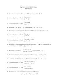
Figure 23.9: A surface generated by applying a rotation curve to a helix

796 CHAPTER 23. ROTATION USING QUATERNIONS
A natural question is what happens when γ is one of the ellipses (23.39).
Figure 23.1 was obtained by taking
9
γ(u) = exp A[(0,
10 cosu, 27
100
sin u)]
in the notation of (23.10), and β to be the straight line
β(v) = (v, 0, 0).
Figure 23.9 applies a similar rotation curve to the space curve
β(v) = ( cos5v, sin 5v, 10v ) .
Rotations in R 4
The astute reader may question the extent to which quaternions are essential for
an analysis of the rotation group. While it is true that Theorem 23.4 provided
the main computational power of the chapter, one should not underestimate
the mathematical significance of Theorem 23.11, particularly in extending the
theory to R n . To finish, we merely state a generalization of Lemma 23.10.
Lemma 23.19. Let q 1 ,q 2 ∈ U . If p ∈ H then q 1 pq 2 is a quaternion with the
same norm as p. The resulting mapping
(23.47)
p ↦→ q 1 pq 2
is an orthogonal transformation of R 4 and determines a matrix in SO(4).
Proof.
It suffices to modify the step (23.25) for the previous proof to work.
This leads to a description of SO(4) based on U × U . Further to (23.30),
there is an associated homomorphism of groups
U × U −→ SO(4).
Exactly two elements of U × U (namely, (q 1 ,q 2 ) and (−q 1 , −q 2 )) map to the
same rotation of R 4 . Elements of the type (q,q) really do map to SO(3), in the
sense that they leave fixed the direction generated by 1 ∈ H, in the same way
that (23.4) is effectively a rotation of R 2 rather than R 3 .
The ability to describe a rotation by two separate elements q 1 ,q 2 is a special
feature of the group of rotations in four dimensions. This led in the 1970s to a
fuller understanding by mathematicians of gauge theories in theoretical physics,
a resurgence of interest in quaternions [Atiyah], and unforeseen developments
in pure mathematics.

23.8. EXERCISES 797
23.8 Exercises
1. Prove that the matrix A = A[x] satisfies
(a) A 3 = −‖x‖ 2 A.
(b) A 2 = xx T − ‖x‖ 2 I 3 .
2. Let p,q ∈ H. Under what conditions on p and q is it true that pq = qp?
3. Show that the eight elements
1, −1, i, j, k, −i, −j, −k
form a group under quaternion multiplication.
4. Let P ∈ SO(3), P 2 ≠ I 3 . Show that P represents a rotation about an axis
parallel to the vector x, where A[x] = P − P T .
5. Prove that if X, Y are skew-symmetric n×n matrices then so is XY −Y X.
Now suppose that n = 3 and that X =A[x], Y =A[y]. Use (23.11) to verify
that
XY − Y X = A[x × y],
and relate this fact to the Jacobi identity (24.46) on page 832.
(
α
6. Let A =
γ
)
β
be a complex 2 ×2 matrix satisfying A T A = I 2 , where
δ
A is the matrix obtained from A by complex-conjugating its four elements
and I 2 is the identity. Show that the complex number detA = αδ − βγ
has modulus one, and that if detA = 1 then γ = −β and δ = α.
7. Prove that the set of matrices
{(
α
SU(2) =
−β
) ∣∣∣∣
β
|α| 2 + |β| 2 = 1}
α
arising from the previous question is a group under matrix multiplication.
By writing each complex entry in real and imaginary parts, show that its
elements are in bijective correspondence with those of the group U of unit
quaternions.
8. Show that a unit quaternion
q = a + bi + cj + dk
can be written as a product q = q 1 q 2 with q 1 ∈ U i and q 2 ∈ U j if and
only if ad − bc = 0. See (23.41) for the notation.

798 CHAPTER 23. ROTATION USING QUATERNIONS
M 9. Plot the projection of the curve (23.46) on the xy-plane, and verify that
it is not a circle. Find analogous expressions for the normal and binormal
vectors to Viviani’s curve.
M 10. Verify the limits (23.45), and plot the rotation curve F(t) for a twisted
cubic.
M 11. Let β: (a, b) → R 3 be a curve with speed v = v(t) whose Frenet frame
defines γ : (a, b) → SO(3). Use Theorem 7.13 to show that
where x(t) = (−τ(t), 0, κ(t))v.
γ ′ (t) = γ(t)A[x(t)],
12. Define an equivalence relation ∼ on S n (1) ⊂ R n+1 by writing a ∼ b if and
only if a = ±b. The resulting quotient space is called real projective space
of dimension n and denoted by RP n . The case n = 2 was the subject of
Section 11.5. Define p: S n (1) ↦→ RP n by p(a) = {a, −a}. Deduce from
Theorem 23.11 that there is a bijective correspondence between SO(3)
and RP 3 .