j - Dipartimento di Matematica - Politecnico di Torino

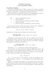
hard copy ISSN 1974-3041
on-line ISSN 1974-305X
La Matematica
e le sue Applicazioni
n. 11, 2010
A mathematical procedure for the evolution of future
landscape scenarios
F. Gobattoni, G. Lauro, A. Leone, R. Monaco, R. Pelorosso
Quaderni del
Dipartimento di Matematica
Politecnico di Torino
Corso Duca degli Abruzzi, 24 – 10129 Torino – Italia

Edizioni C.L.U.T. - Torino
Corso Duca degli Abruzzi, 24
10129 Torino
Tel. 011 564 79 80 - Fax. 011 54 21 92
La Matematica e le sue Applicazioni
hard copy ISSN 1974-3041
on-line ISSN 1974-305X
Direttore: Claudio Canuto
Comitato editoriale: N. Bellomo, C. Canuto, G. Casnati, M. Gasparini, R. Monaco,
G. Monegato, L. Pandolfi, G. Pistone, S. Salamon, E. Serra, A. Tabacco
Esemplare fuori commercio
accettato nel mese di Ottobre 2010

A mathematical procedure for the evolution of future landscape scenarios.
Authors: F. Gobattoni 1 , G. Lauro 2 , A. Leone 1 , R. Monaco 3 , R. Pelorosso 1
1 Department of Environment and Forestry, University of Tuscia, Viterbo (Italy)
2 Architecture Faculty, Second University of Naples, 81031 Aversa, (Italy)
3 Department of Mathematics, Politecnico di Torino, Torino (Italy)
Corresponding author: f.gobattoni@unitus.it
Introduction
Since the European Landscape Convention aims to encourage all European countries to define their
landscape quality objectives, a new frame of mind in management and planning of territory is
nowadays required as a point of reference for territorial government, entities and authorities, so as
to advance towards conservation and protection of landscapes providing positive impact on the
quality of life of population. Moreover, planning efficiently at the landscape scale needs a crosssector
cooperation and people involvement with planners and communities working closely in
achieving positive landscape change understanding and in characterizing the relations between
nature and society, which will integrate landscapes and their dynamics. (C. Petit et al., 2008).
The methodologies for successful landscape and environmental planning have been severely
challenged when classical concepts and models such as economic and socioeconomic development,
ecosystems preservation and sustainability have been questioned (J. E. Vermaat et al., 2005). The
actual challenge is to build transparent and flexible decision-making tools to be used in
environmental planning and to embrace a broad range of stakeholders needs together with
landscape management requirements.
Landscape-scale geographical information provides an ideal framework for developing spatial
strategies and to implement simulation models to support landscape planning identifying
opportunities for change and anticipating and comparing the results of planning decisions. Model
outputs can be used to elaborate thematic maps and visualizations of landscape scenarios as an
effective and direct way of communicating results and opportunities.
In this framework, landscapes can be defined as spatially extended heterogenous complex systems
organized hierarchically into structural arrangements determined by nonlinear interactions among
their components through flows of energy and materials (we shall use the overall term "bio-energy"
as introduced by Ingegnoli, 2002 ). Human activity has, also, strongly modified recent landscape by
means of land use and land cover changes and consuming of natural resources (Pelorosso et al.,
2009). Alterations of natural equilibriums has pointed out several consequences on landscape
capacity to furnish goods and service (Willemen et al, 2008) as biodiversity conservation
(Tscharntke et al., 2005) and regulation of water regimes (Lindborg et al., 2008).
Environmental available energy has been pointed out as a key factor in the explanation of many
ecological processes and theories (metabolic and species energy theory, biodiversity conservation)
recurring to different indeces (e.g. Net Primary Productivity, NNP, Actual Evapotraspiration, AET,
Potential Evapotraspiration, PET) (Hurlbert and Jetz, 2010; Currie, 1991; Carrara et al. 2010;
Brown at al., 2004). A more complete measure of available energy, so-called Biological Territorial
Capacity (BTC), was proposed by Ingegnoli (2002) considering a synthetic function of vegetation
metabolism. As the importance of energy exchange, although it is rare for a landscape to be in any
form of equilibrium and the landscape equilibrium concept is not yet clear (Perry, 2002; Turner et
al., 1993; Bracken and Wainwright, 2006), it’s interesting to focus on which hypothetical energetic
equilibrium state is going to be realized and the effects of human decisions on that equilibrium.
Most of mathematical models are strictly related to air dispersion, hydrology and hydrodynamics,
water quality, ground water quality, erosion and sedimentation, and so on, just taking into account
each aspect of the environmental system separately and without looking directly at landscape as a

unique system and without understanding its intrinsic evolution mechanisms. All decision making
involves an implicit (if not explicit) use of models, since the decision maker invariably has a causal
relationship in mind when he makes a decision. So mathematical models able to explain the
landscape evolution and to compare the effects of future scenarios on its evolution and equilibrium
in time, are really needed not also to understand environmental system mechanism and behaviour
but above all to better plan strategies for natural resources conservation management and landscape
preservation.
The environment is here considered as composed by several Landscape Units (LU) delimited by
natural and/or anthropic barriers. An integrated GIS (Geographic Information System)-based
approach was developed (G. Lauro, R. Monaco, 2008) combining an ecological graph model for the
analysis of the relationship between spatial pattern and ecological fluxes and a mathematical model,
based on a system of two nonlinear differential equations. These equations are mainly based on a
balance law between a logistic growth of bio-energy and its reduction due to limiting factors
coming from environmental constraints. The energy exchange among them will be more or less
strong depending on the degree of permeability of the barriers which can obstruct the energy
passage from each LU to the other.
A GIS-based mathematical model, based on the ecological graph and on the cited two differential
equations, is presented and discussed here. A study case in Central Italy is introduced and discussed
here just to show the importance of a such mathematical procedure to figure out planning strategies
and environmental conservation and management actions with the support of rigorous methods able
to fix and compare the effects of anthropic decisions on landscape.
Study area description
The study area (Fig. 1) for the model development, is Traponzo River catchment; Traponzo River is
located in the northern part of Lazio Region and its watershed covers part of nine municipalities,
lying completely in the Province of Viterbo.
This stream originates in Monti Cimini relief and flows into Marta river so that Traponzo
catchment, as a sub-basin of Marta river, has a total area of 475 Km 2 , with a mean elevation of 526
m a.s.l. and a maximum of 979 m a.s.l.. The climate of this area is quite Mediterranean with a mean
annual temperature of about 15°C and a mean annual precipitation of about 970 mm. The total area
covered by urban sprawl is about 2.23 km 2 that is about 10% of the total urban area.
Land cover class Area (km 2 ) %
Urban 21.02 4.4
Forest 126.36 26.6
Non irrigated crops 203.04 42.8
Pasture 22.01 4.6
Orchards 88.17 18.6
Irrigated crops 2.49 0.5
Hedges 11.77 2.5
Water bodies 0.02 0
Total area 474.89 100
Table 1.

Fig.1. Study area

Model description and methodologies
Gathering all the available information on the climatic, topographic, land cover, geological and
pedological characteristics describing our study area, a GIS dataset has been created not only to
represent the watershed but also to identify and derive the LU structure. Taking into account urban
areas distribution, primary and secondary roads network, soil features and elevation and weighting
them through the application of Saaty matrix, a standard heuristic methodology has been fixed to
split the study area into well defined LU. A number of 46 LU has been derived for this study area
and an ecological graph for representing the energy flows between them has been elaborated taking
into account the Biological Territorial Capacity (BTC) proposed by Ingegnoli (2002). The
ecological graph, at first introduced by Fabbri (2003), has been applied here to quantify and
correlate the energy production from a landscape unit as a flow of energy to its neighbours
according to the permeability of the boundaries.
The study area GIS dataset also allow to set up all the parameters needed to run the mathematical
model structured as follows.
It consists in two ordinary differential equations, of evolution in time, of the following two state
variables, M(t) and V(t) :
1) M(t), the mean value of the biological energy of the whole system, t being the time, given by
m
1
M ( t)
= ∑ M j
, M j = (1 + Kj)Bj (1), (2)
m
j=
1
where Bj is an index measuring the BTC of the j LU, that is the magnitude representing the energy
(Mcal/m 2 /year) that system needs to dissipate in order to maintain its equilibrium state and its
organizational level, and where the parameter Kj depends on several properties related to unit’s
composition. In particular, in this paper we shall consider that it depends on 5 features and it is
given by
F P D C E
K = ( K + K + K + K + K ) / 5
(3)
j
where
j
j
j
j
j
F
K
j
takes into account the shape of the patch borders,
P
K
j
their permeability,
D
K
j
the bio-
C
E
diversity of the LU. The last two parameters K
j
and K
j
are related, respectively, to the relative
humidity of the soil and to the sun exposition of the LU, and are introduced for the first time in this
paper. We recall that all these parameters are defined in such a way that K ∈ [0; 1].
For the computation of the parameters
Conversely
K
C
j
w1
A
=
h
j
C
K
j
and
+ w
A
j
2
A
s
j
F
K
j
,
P
K
j
and
E
K
j
are defined by the following formulae:
, K
where the w k are suitable weights,
E
j
SWE W
3
Aj
+ w4
Aj
+
j
D
K
j
, see Finotto et al. (2010).
NE
w
w5
Aj
= (4), (5)
A
Aj
is the total area of the j LU, and
j
h s
A
j
, A
j
,
SWE
A
j
,
W
A
j
,
are the fractions of soil surfaces characterized by humidity, sub-humidity, south-west-east, west and
north-west exposition.
Moreover:
M = , B max { B }
max
2B max
max
= (6), (7)
j=
1,...., m
j
NE
A
j

in other words M max is the maximum value of biological energy that the environment under
consideration can exhibit according to the maximum value of bio-potentiality expressed by the m
different LU. These last definitions lead to fix the bio-potentiality index as
B
b T
= (8)
B max
which, thus, turns out to be confined in the range [0; 1].
2) V (t), the fraction of the total territory’s surface occupied by areas characterized by high values
of Bj ( high values correspond, for example, to wooden areas).
The proposed equations read :
' ⎡ M ( t)
⎤
M ( t)
= cM ( t)
⎢1
− − k[ 1 −V
( t)
] M ( t),
M
⎥
(9)
⎣ max ⎦
[ 1 −V
( t)
] h U V ( ),
V ' ( t)
= bTV
( t)
−
0 0
t
(10)
They read as a balance law between a logistic growth of bio-energy M (t) and its reduction due to
limiting factors coming from environmental constraints expressed by the coefficients c, k, b T , h,
Uo.
Having already given the definition of b T , we now proceed to deal with the other parameters.
c∈ [0; 1] is the connectivity index which is a function of the energy fluxes F ij between each pair of
confining LU, namely
S S
Mi
+ M
j
Fij
=
2
Lij
⋅ ⋅ p
P + P
i
j
(11)
L ij being the length of the boundary between the i and j LU; P i and P j being their perimeters, while
p is the permeability index of such a boundary. Moreover k is the ratio between the sum of the
perimeters of the impermeable barriers and the perimeter of the whole environment. h is another
environment impact parameter defined as the ratio between the sum of the edified areas perimeter
(both compact and spread) and the total perimeter P of the whole environment. Finally U 0 ∈ [0; 1]
is the ratio between the surface of the edified areas and the total area S of the system. U 0 will be
computed as the weighted average:
U
0
w6U
c
+ w7U
s
= (12)
S
where U c and U s are the surface fractions of compact and spread edified areas, and w 6 , w 7 suitable
weights. Note that conversely to the other parameters of the model, k and h may assume values
greater than one (Finotto et al., 2010).
In order to get a detailed evolution of the environment, one can integrate the equations (9-10) from
suitable initial data M(0) and V(0) which can be recovered by the ecological graph. The model
provide these scenarios corresponding to the following four equilibrium solutions of the differential
equation system:

(1)
(1)
(a) M = 0 ; V = 0
(2)
(b) M = 0 ;
( 2) bT
− hU
0
V
=
b
T
(c)
(d)
M
M
M
max
( c k)
(3)
= , V = 0
c
( 3) −
(4)
=
M
max
[ c − k( 1 −V
)]
c
e
,
b
=
hU
b
( 4) T
−
0
V
T
As it can be easily understood the first equilibrium is quite negative since it prevents an
environment where production and diffusion of biological energy is negligible and no areas of high
ecological quality are present. The second scenario is that of a territory strongly fragmented where
diffusion of biological energy between the LU is again negligible but some area of high quality
vegetation is still present. The third equilibrium corresponds to a territory characterized by some
production and diffusion of bio-energy but low vegetation quality. Finally the last scenario is that
more favourable since strong production and diffusion of biological energy between the LU allows
to guarantee an ecological settlement of high level of bio-potentiality. The stability analysis (Finotto
et al., 2010) has shown that the above equilibrium solutions can be obtained, respectively, when the
model parameters satisfy the following inequalities:
c < k and b T
< hU
0
(I)
khU
0
> cb T
and b T
> hU
0
(II)
c > k and b T
< hU
0
(III)
khU
0
> cb T
and b T
> hU
0
(IV)
The ecological graph representation together with the solutions of the mathematical procedure can
be derived through a NetLogo model application that give us an easy tool to model the equilibrium
states of landscape evolution starting from the initial, actual conditions as described by the
ecological graph itself (Gobattoni F. et al., 2010).
Results and discussion
As an assessment of the ecological behaviour for an environment, the ecological graph assigns a
node dimension proportional to the available energy and a link between LU with a dimension
proportional to the flux of energy. The energy exchange among them will be more or less strong
depending on the degree of permeability of the barriers which can obstruct the energy passage from
each LU to the other.

Fig. 2 Ecological graph representation for the study area.

Applying the proposed LU identification methodology and deriving all the required parameters
needed to set up the mathematical model, this summarizing table can be obtained:
Total area (km 2 ) 475
High bio-potentiality area (km 2 ) 124
V 0 0.26
b T 0.1606
M max (Mcal/m 2 /year) 2.3 E+08
B max (Mcal/m 2 /year) 1.5 E+08
U 0 0.02
h 1.96
k 0.75
c 0.0374
V e 0.72
M e 0
Table 2.
The values in Table 2, have been entered in NetLogo model elaborating the proposed differential
system. In particular, b
T
, h, U
0
, M max , k and c seems to satisfy the inequality (II) so that the
equilibrium corresponding to he second scenario turns out to be stable and the system evolves
asymptotically to this equilibrium state. The system tends to keep areas with high value of biopotentiality
but they are isolated in landscape pattern and the fluxes of bio-energy between them
seem to be limited. As a consequence, the dynamic evolution of this environmental system shows a
trend toward a good production of bio-energy but with a limited diffusion of it, and, then, with
limited fluxes between LU. A low connectivity index (Table 2), discloses to this equilibrium state
as a solution of the differential equations system, since the lack of connectivity prejudices the
energy exchange between LU even containing high BTC values areas. The landscape fragmentation
provoked by a large urban sprawl phenomenon and by the rich and structured roads network is
reflected on the confined and obstructed energy fluxes between LU. The need of opportune
planning strategies and actions to reduce fragmentation favouring the energy fluxes between
ecosystems and preserving biodiversity, has to be underlined since the actual landscape pattern for
the study area shows a low response in terms of connectivity and energy fluxes.
Conclusions
If the ecological graph is a powerful tool to represent connections efficiency between LU and to
identify high ecological values areas to be protected and compromised ones limiting energy fluxes,
on the other side a mathematical model evaluating the potential effectiveness of natural resources
on the long term, is essential to assess the diachronic evolution of landscape as a unique system.
An integrated approach combining the ecological graph and the mathematical model, allows to face
the great challenge of planning and management under sustainable environmental and economical
conditions since it can represent a powerful decision system support to compare effects and impacts
of alternative scenarios and actions (evaluation of new roads and urban development plans).
Not only for a description of the available energy at LU scale but also as a tool for evaluating the
equilibrium trend in landscape evolution, this mathematical and GIS interfaced method can help in
understanding environment response and dynamic change in time to correctly manage and preserve
natural resources and ecosystems.

References
Bracken L. J and Wainwright J. 2006. Geomorphological equilibrium: myth and metaphor? Trans
Inst Br Geogr, 31:167–178.
Brown J. H., Gillooly J. F., Allen A. P., Savage V. M., West G. B. 2004. Toward a Metabolic
Theory of Ecology. Ecology, 85(4):1771-1789.
Carrara R. and Vàzquez D. P. 2010. The species energy theory: a role for energy variability.
Ecography 000: 000000 doi: 10.1111/j.1600-0587.2009.05756.x.
Currie D. J. 1991. Energy and large-scale patterns of Animal- and Plant-Species Richness. The
American Naturalist, 137:27-49.
Fabbri P., Paesaggio, Pianificazione, Sostenibilità, Alinea Editrice, Firenze 2003. Principi
Ecologici per la Progettazione del Paesaggio, Franco Angeli, Milano 2007.
Finotto F., Monaco R., Servente G., Un modello per la valutazione della produzione e della
diffusività di energia biologica in un sistema ambientale, to be printed on Scienze Regionali (Ital. J.
of Regional Sci.), 2010.
Forman R. T. T. 1995. Land Mosaics. The ecology of landscape and regions. Cambridge:
Cambridge Press.
Gobattoni F., Lauro G., Leone A., Monaco R., Pelorosso R., 2010. A simulation method for the
stability analysis of landscape scenarios by using a NetLogo application in GIS environment. EGU
Conference, 3-7 May, Vienna, Austria.
Hurlbert A. H. and Jetz W. 2010. More than “More Individuals”: The Non-equivalence of Area and
Energy in the Scaling of Species Richness. Am Nat 2010. Vol. 176, pp. 000–000 DOI:
10.1086/650723.
Ingegnoli V. 2002. Landscape Ecology: A Widening Foundation. New York-Berlin: Springer-
Verlag.
Ingegnoli V., Forman R.F., 2002. Landscape Ecology: A Widening Foundation, Springer-Werlag,
New York.
Lauro G., Lisi M., Monaco R., 2008. Bifurcation analysis of a dynamical model for an ecological
system. La Matematica e le sue Applicazioni, n. 15. on-line ISSN 1974-305X.
Naveh Z., Liebermann A. 1984. Landscape ecology: theory and application. Springer-Werlag, New
York.
Pelorosso R., Leone A., Boccia L. 2009. Land cover and land use change in the Italian central
Apennines: A comparison of assessment methods. Applied Geography 29:35–48.
Perry L.W., 2002. Landscape, space and equilibrium: shifting viewpoints. Progress in Physical
Geography, 26 (3):339-359.
Petit C.et al., 2008. Landscape Analysis and Visualisation-Spatial Models for Natural Resources
and Planning. Springer,
Tscharntke T., Klein A. M., Kruess A., Steffan-Dewenter I.and Thies C. 2005. Landscape
perspectives on agricultural intensification and biodiversity – ecosystem service management.
Ecology Letters, 8 (8):857-874.
Turner M. G., Romme W. H., Gardnerl R. H., O’Neill R. V. and Kratz T. K. 1993. A revised
concept of landscape equilibrium: Disturbance and stability on scaled landscapes. Landscape
Ecology, 8(3):213-227.
Turner M.G., Gardner R.H., 1990. Quantitative methods in Landscape Ecology. Springer-Werlag,
New York.
Vermaat, J.E., Eppink, F., Van den Bergh, J.C.J.M., Barendregt, A. & Van Belle, J. 2005. Matching
of scales in spatial economic and ecological analysis. Ecol. Econ., 52, 229-237.
Willemen L., Verburg P.H., Hein L., Van Mensvoort M. E. F. (2008). Spatial characterization of
landscape functions. Landscape and Urban Planning, 88:34-43.