Addition of Angular Momenta
Addition of Angular Momenta
Addition of Angular Momenta

Create successful ePaper yourself
Turn your PDF publications into a flip-book with our unique Google optimized e-Paper software.
<strong>Addition</strong> <strong>of</strong> <strong>Angular</strong> <strong>Momenta</strong><br />
What we have so far considered to be an ’exact’ solution for the many electron problem,<br />
should really be called ’exact non-relativistic’ solution. A relativistic treatment is needed<br />
to properly introduce spin and a relativistic term in the Hamiltonian then also appears,<br />
the so-called spin-orbit coupling. While this is a rather small correction for most atoms,<br />
especially the smaller ones, it is important to be aware <strong>of</strong> this. Most importantly, it means<br />
that the total orbital angular momentum and the total spin are no longer constants <strong>of</strong> the<br />
motion, i.e. conserved quantities that can be used to characterize the system. This is an<br />
example <strong>of</strong> the problem <strong>of</strong> ’adding angular momenta’ in quantum mechanics.<br />
Constants <strong>of</strong> the Motion<br />
It is particularly valuable to know any property <strong>of</strong> the system that does not change<br />
with time. Such properties are called ’constants <strong>of</strong> the motion’. One example is the total<br />
energy. For a closed system, the total energy is a constant. The angular momentum <strong>of</strong><br />
a rotating, classical object is another example. In a system <strong>of</strong> two or more interacting<br />
objects, it is the total angular momentum that is conserved. As mentioned above, for an<br />
electron in an atoms, one needs to add the angular momentum due to the motion <strong>of</strong> the<br />
electron around the nucleus <strong>of</strong> the atom and the angular momentum due to the spin <strong>of</strong> the<br />
electron to get the total angular momentum, which is conserved. Identifying such constants<br />
<strong>of</strong> the motion is important whether one is dealing with classical mechanics or quantum<br />
mechanics. In quantum mechanics it is, furthermore, useful to work with eigenfunctions <strong>of</strong><br />
operators that correspond to constants <strong>of</strong> the motion. Such operators commute with the<br />
Hamiltonian as can be seen from the following calculation.<br />
The expectation value <strong>of</strong> an arbitrary operator Ω has time dependence:<br />
d<br />
dt < ψ∣ ∣<br />
∣ Ω∣ψ> d < ψ| =<br />
dt<br />
where d|ψ><br />
and<br />
dt<br />
d < ψ|<br />
dt<br />
= 1<br />
i¯h H∣ ∣ ψ><br />
= 1<br />
−i¯h < ψ∣ ∣ H.<br />
Ω ∣ ∣ ψ> + < ψ dΩ<br />
∣<br />
∣ ψ> + < ψ∣Ω d|ψ><br />
dt<br />
dt<br />
When the operator, Ω, itself is not explicitly time dependent, the middle term vanishes,<br />
dΩ/dt = 0. Then<br />
d<br />
dt < ψ∣ ∣<br />
∣ Ω∣ψ>= i<br />
¯h < ψ∣ ∣<br />
∣ HΩ − ΩH∣ψ> .<br />
The observable < ψ|Ω|ψ> is, therefore, a constant <strong>of</strong> the motion if [H, Ω] = 0.<br />
As an example, the orbital angular momentum L ⃗ <strong>of</strong> an electron in a spherically symmetric<br />
potential (such as an electron interacting with a heavy nucleus) satisfies [H, L] ⃗ = 0<br />
and, therefore, is a constant <strong>of</strong> the motion. It is natural to use the eigenfunctions <strong>of</strong> L, ⃗<br />
the spherical harmonics Yl m (θ, φ), to represent the (θ, φ) dependence. The r dependence<br />
separates and we are left with solving a one-dimensional problem. Recall the discussion <strong>of</strong><br />
the hydrogen-like atoms.<br />
23
When two angular momenta are present and when there is an interaction between<br />
them, then each one separately will not be a constant <strong>of</strong> the motion. It is then advantageous<br />
to define a new vector, the total angular momentum, which in the absence <strong>of</strong> external<br />
perturbations, is a constant <strong>of</strong> the motion. Following is a discussion <strong>of</strong> two simple but<br />
important examples that illustrate this.<br />
Example 1: Two particles interacting via spherically symmetric potential (for example<br />
the two electrons in a He atom).<br />
The Hamiltonian is<br />
H = H 1 + H 2 + v<br />
where<br />
H 1 = − ¯h2<br />
2m ∇2 1 + V (r 1)<br />
H 2 = − ¯h2<br />
2m ∇2 2 + V (r 2)<br />
v = v(r 12 ) = v(|⃗r 2 − ⃗r 1 |).<br />
We are assuming that each particle is in a force field with spherical symmetry,<br />
V (r 1 ) = V (|⃗r 1 |) and V (r 2 ) = V (|⃗r 2 |).<br />
Therefore, the orbital angular momentum and the Hamiltonian for each particle commute<br />
[L 1 , H 1 ] = [L 2 , H 2 ] = 0.<br />
We also have<br />
[L 1 , H 2 ] = [L 2 , H 1 ] = 0<br />
(L 1 and H 2 act on different variables, and similarly L 2 and H 1 ). Therefore, the individual<br />
angular momenta L 1 and L 2 would be constants <strong>of</strong> the motion, i.e. [L 1 , H] = [L 2 , H] = 0,<br />
if the interaction v(r 12 ) were absent.<br />
Even when the interaction, v, is present, a combination <strong>of</strong> ⃗ L 1 and ⃗ L 2 can be found<br />
that is a constant <strong>of</strong> the motion as long as v only depends on the scalar distance between<br />
the particles<br />
r 12 = |⃗r 1 − ⃗r 2 | = √ (x 1 − x 2 ) 2 + (y 1 − y 2 ) 2 + (z 1 − z 2 ) 2 .<br />
Find: [L 1z , H]:<br />
Using the definition <strong>of</strong> L 1z<br />
L 1z = ¯h i (x ∂ ∂<br />
1 − y 1 )<br />
∂y 1 ∂x 1<br />
24
and the product rule for differentiation gives<br />
[L 1z , H] ψ(⃗r 1 ,⃗r 2 ) = [L 1z , v] ψ = L 1z vψ − vL 1z ψ<br />
= ¯h (<br />
)<br />
∂(vψ) ∂(vψ)<br />
x 1 − y 1 − v¯h (<br />
)<br />
∂ψ ∂ψ<br />
x 1 − y 1<br />
i ∂y 1 ∂x 1 i ∂y 1 ∂x 1<br />
= ¯h (<br />
∂v<br />
x 1 ψ + x 1 v ∂ψ ∂v<br />
− y 1 ψ − y 1 v ∂ψ − x 1 v ∂ψ + y 1 v ∂ψ )<br />
i ∂y 1 ∂y 1 ∂x 1 ∂x 1 ∂y 1 ∂x 1<br />
= ¯h (<br />
)<br />
∂v ∂v<br />
x 1 − y 1 ψ(⃗r 1 ,⃗r 2 )<br />
i ∂y 1 ∂x 1<br />
= ¯h (<br />
)<br />
y 1 − y 2<br />
x 1 v ′ x 1 − x 2<br />
(r 12 ) − y 1 v ′ (r 12 ) ψ(⃗r 1 ,⃗r 2 )<br />
i r 12 r 12<br />
= ¯h i (y 1x 2 − x 1 y 2 ) v′ (r 12 )<br />
ψ(⃗r 1 ,⃗r 2 ).<br />
r 12<br />
The derivatives <strong>of</strong> v can be found using the chain rule<br />
∂v(r 12 )<br />
∂y 1<br />
= ∂r 12<br />
∂y 1<br />
∂v(r 12 )<br />
∂r 12<br />
= y 1 − y 2<br />
r 12<br />
v ′ (r 12 )<br />
with v ′ denoting the derivative <strong>of</strong> the potential function v(α) with respect to the argument<br />
α. Therefore, in operator form,<br />
[<br />
L1z , H ] = ¯h i (Y 1X 2 − X 1 Y 2 ) v′ (r 12 )<br />
r 12<br />
≠ 0.<br />
When the interaction v(r 12 ) is present, L 1z is no longer a constant <strong>of</strong> the motion. Similarly,<br />
[<br />
L2z , H ] = ¯h i (Y 2X 1 − X 2 Y 1 ) v′ (r 12 )<br />
r 12<br />
.<br />
However, if the two results are added together to obtain a commutator for L 1z + L 2z<br />
[<br />
L1z + L 2z , H ] = ¯h v(r 12 )<br />
(Y 1 X 2 − X 1 Y 2 + Y 2 X 1 − X 2 Y 1 )<br />
i r 12<br />
= 0.<br />
The sum L 1z + L 2z is a constant <strong>of</strong> the motion. Similarly we could show that L 1y + L 2y<br />
and L 1x + L 2x are also constants <strong>of</strong> the motion. Therefore, we can define a new vector<br />
⃗L ≡ ⃗ L 1 + ⃗ L 2 which is a constant <strong>of</strong> the motion. The commutation relations for the<br />
25
components <strong>of</strong> this new vector are<br />
[L x , L y ] = [L 1x + L 2x , L 1y + L 2y ]<br />
and, similarly,<br />
= [L 1x , L 1y ] + [L 1x , L 2y ] + [L 2x , L 1y ] + [L 2x , L 2y ]<br />
= i¯h L 1z + i¯h L 2z<br />
= i¯h L z<br />
[L y , L z ] = i¯h L x<br />
and<br />
[L z , L x ] = i¯h L y .<br />
So, by definition, ⃗ L is an angular momentum. It is the total angular momentum. If the two<br />
particles start out in an eigenstate <strong>of</strong> ⃗ L, they will remain in that state unless the system<br />
is perturbed. The problem <strong>of</strong> ’adding angular momenta’ involves finding those states in<br />
terms <strong>of</strong> the eigenstates <strong>of</strong> ⃗ L 1 and ⃗ L 2 .<br />
In classical mechanics the situation is analogous. Total angular momentum <strong>of</strong> two<br />
interacting particles is constant but not the angular momentum <strong>of</strong> each particle separately<br />
if the two interact. But, we usually do not have the problem <strong>of</strong> basis set transformations<br />
in classical mechanics.<br />
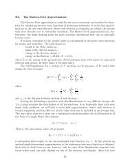
Example 2: A particle with spin moving in a central potential v(r) in the presence <strong>of</strong><br />
spin-orbit coupling.<br />
First <strong>of</strong> all, if the Hamiltonian is simply<br />
H = − ¯h2<br />
2m ∇2 + v(r)<br />
then [ ⃗ L, H] = 0 and [ ⃗ S, H] = 0. That is, the two angular momenta are separately constants<br />
<strong>of</strong> the motion if the Hamiltonian does not couple ⃗ L and ⃗ S.<br />
But in relativistic quantum mechanics the spin and orbital angular momenta turn out<br />
to be interacting, or, equivalently, they are coupled together. The interaction is called<br />
spin-orbit coupling and has the form<br />
⃗L · ⃗S = L x S x + L y S y + L z S z .<br />
In the electronic states <strong>of</strong> atoms, this leads to the various terms and term symbols which<br />
are a more rigorous description <strong>of</strong> the state <strong>of</strong> the atom than electron configuration. The<br />
electron configuration does not take into account spin-orbit coupling. It turns out that<br />
the coupling strength is a function <strong>of</strong> the distance to the origin, ζ(r). Thus, the full<br />
Hamiltonian including spin-orbit coupling can be written as<br />
H = − ¯h2<br />
2m ∇2 + v(r) + ζ(r) ⃗ L · ⃗S.<br />
26
Due to the spin-orbit coupling the orbital angular momentum ⃗ L is no longer a constant<br />
<strong>of</strong> the motion. The commutator for the z component, for example, is<br />
[L z , H] = ζ [L z , L x S x + L y S y + L z S z ]<br />
= ζ (S x [L z , L x ] + S y [L z , L y ] + S z [L z , L z ])<br />
= ζ (S x i¯hL y + S y (−i¯hL x ))<br />
= ζ i¯h(S x L y − S y L x )<br />
≠ 0<br />
Similarly, the spin ⃗ S is no longer a constant <strong>of</strong> the motion.<br />
[S z , H] = ζ i¯h(L x S y − L y S x )<br />
≠ 0.<br />
However, the z-component <strong>of</strong> the sum <strong>of</strong> the two angular momentum vectors, ⃗ L z + ⃗ S z ,<br />
is a constant <strong>of</strong> the motion as can be seen by adding the two commutators above,<br />
[L z + S z , H] = 0.<br />
Similar calculation can be done for the x and y components. Therefore, the total angular<br />
momentum ⃗ J ≡ ⃗ L + ⃗ S is a constant <strong>of</strong> the motion. Again, we can easily show that ⃗ J<br />
satisfies the commutation relations that define an angular momentum vector<br />
[J x , J y ] = i¯hJ z , etc.<br />
The Hamiltonians in examples 1 and 2 are common. Working with the eigenstates <strong>of</strong><br />
the total angular momentum rather than the eigenstates <strong>of</strong> the individual angular momenta<br />
greatly simplifies calculations is such cases. The problem <strong>of</strong> ‘addition <strong>of</strong> angular momenta’<br />
therefore involves more than just addition <strong>of</strong> two vectors, we need to find the eigenstates <strong>of</strong><br />
the total angular momentum and express them in terms <strong>of</strong> the already known eigenstates<br />
<strong>of</strong> the individual angular momenta.<br />
Definition <strong>of</strong> Clebsch-Gordan coefficients:<br />
The general problem can be stated in the following way: Given two angular momenta<br />
L ⃗ and S ⃗ (not necessarily orbital and spin angular momenta, here L ⃗ and S ⃗ are<br />
used as general symbols for any two angular momenta) and their eigenkets |lm l > and<br />
|sm s >, a complete set <strong>of</strong> eigenkets for the combined system can be constructed by direct<br />
multiplication<br />
|lsm l m s >≡ |lm l > ⊗|sm s > .<br />
This is a complete set and forms a basis but these kets do not correspond to a constant<br />
<strong>of</strong> the motion. Instead, one would like to transform to a new set <strong>of</strong> kets |jm > that<br />
27
correspond to eigenstates <strong>of</strong> J 2 , J z , L 2 and S 2 where the total angular momentum is<br />
defined as ⃗ J ≡ ⃗ L + ⃗ S. That is, the new kets should satisfy<br />
J 2 |jm>= j(j + 1)¯h 2 |jm><br />
J z |jm>= m¯h|jm><br />
L 2 |jm>= l(l + 1)¯h 2 |jm><br />
and<br />
S 2 |jm>= s(s + 1)¯h 2 |jm> .<br />
The new vectors can be constructed from the direct product basis<br />
|jm>=<br />
l∑<br />
s∑<br />
m l =−l m s =−s<br />
a lsml m s ;jm|lsm l m s ><br />
and the problem reduces to finding the linear combination coefficients a lsml m s ;jm =<<br />
lsm l m s |jm> which are called Clebsch-Gordan coefficients. They have been tabulated in<br />
may books and are also preprogrammed in various mathematical s<strong>of</strong>tware packages.<br />
Solution for Two Spin 1/2 Particles:<br />
The general method for finding eigenstates <strong>of</strong> the total angular momentum is a bit<br />
involved and it is worthwhile to illustrate the essence <strong>of</strong> the problem in the simple but<br />
important case <strong>of</strong> two spin 1 angular momenta. Here a straight forward application <strong>of</strong><br />
2<br />
linear algebra will do the job. Later, this same problem will be solved using the general<br />
method, and finally the general solution will be presented.<br />
The total spin angular momentum is S ⃗ ≡ S ⃗ 1 + S ⃗ 2 . We want to find a set <strong>of</strong> states<br />
|sm > such that S ⃗2 |sm >= s(s + 1)¯h 2 |sm > and S z |sm >= m¯h|sm >. We will express<br />
them as linear combinations <strong>of</strong> the direct products <strong>of</strong> eigenstates <strong>of</strong> S ⃗ 1 and eigenstates <strong>of</strong><br />
⃗S 2 :<br />
|sm>= a | + +> + b | + −> + c | − +> + d | − −> .<br />
The direct product states satisfy<br />
S 1z | + +> = ¯h 2 | + +><br />
S 1z | + −> = ¯h 2 | + −><br />
S 1z | − +> = −¯h 2 | − +><br />
S 1z | − −> = −¯h 2 | − −><br />
28
and similar relationships for S 2z . The length <strong>of</strong> the two spin vectors is necessarily the same<br />
S 2 1| ± ±> = S 2 2| ± ±> = 3¯h2<br />
4 | ± ±> .<br />
Using the direct product states as basis (in the same order as above), the state |sm><br />
can be expressed in vector notation as<br />
⎛ ⎞<br />
a<br />
⎜ b ⎟<br />
|sm>= ⎝ ⎠.<br />
c<br />
d<br />
First, we will find 4x4 matrices representing the operators S 2 and S z and then by<br />
diagonalizing, get the eigenvectors |sm>.<br />
Matrix for S z :<br />
We need to evaluate all the matrix elements <strong>of</strong> S z in this basis.<br />
⎛<br />
⎞<br />
< + + |S z | + +> < + + |S z | + −> < + + |S z | − +> < + + |S z | − −><br />
⎜ < + − |S<br />
S z =<br />
z | + +> < + − |S z | + −> . . . . . . ⎟<br />
⎝<br />
⎠ .<br />
< − + |S z | + +> . . . . . . . . .<br />
< − − |S z | + +> . . . . . . < − − |S z | − −><br />
First, applying the operator to | + + ><br />
the first column is<br />
S z | + +>= S 1z | + +> +S 2z | + +>=<br />
< + + |S z | + +> = ¯h<br />
< + − |S z | + +> = 0<br />
< − + |S z | + +> = 0<br />
< − − |S z | + +> = 0.<br />
The second and third columns only have zeros because<br />
(¯h<br />
S z | + −> =<br />
2 − ¯h | + −>= 0<br />
2)<br />
and<br />
S z | − +> =<br />
(<br />
−¯h 2 + ¯h )<br />
2<br />
(¯h<br />
2 + ¯h 2)<br />
| + +>= ¯h| + +><br />
| − +>= 0.<br />
The fourth column has one non-zero element just like the first column,<br />
(<br />
S z | − −> = −¯h 2 − ¯h )<br />
| − −>= −¯h | − −> .<br />
2<br />
29
The full matrix is<br />
⎛ ⎞<br />
¯h 0 0 0<br />
⎜ 0 0 0 0 ⎟<br />
S z = ⎝ ⎠ .<br />
0 0 0 0<br />
0 0 0 −¯h<br />
This is already diagonal, i.e., the basis vectors | ± ±> are eigenvectors <strong>of</strong> S z . Any linear<br />
combination that only mixes the | + −> and | − +> vectors will also be an eigenvector.<br />
Matrix for S 2 :<br />
By definition <strong>of</strong> the total angular momentum, we have<br />
S 2 = ⃗ S · ⃗S = ( ⃗ S 1 + ⃗ S 2 ) · ( ⃗ S 1 + ⃗ S 2 ) = S 2 1 + S2 2 + 2⃗ S 1 · ⃗S 2 .<br />
The action <strong>of</strong> the S 2 1 and S 2 2 operators can be readily evaluated but we need a convenient<br />
expression for ⃗ S 1 · ⃗S 2 so that the action <strong>of</strong> this operator on the direct basis functions can<br />
be evaluated. Written in terms <strong>of</strong> the Cartesian components<br />
⃗S 1 · ⃗S 2 = S 1x S 2x + S 1y S 2y + S 1z S 2z<br />
The action <strong>of</strong> the last term, S 1z S 2z , on the direct product states can easily be evaluated, but<br />
the first two terms involving the x and y components are not as straight forward because<br />
the direct product states are not eigenstates <strong>of</strong> those operators. Since we have chosen to<br />
know the projection <strong>of</strong> the spin on the z-axis, the projection onto the y− and x−axes is<br />
not known. It is convenient here to make use <strong>of</strong> the raising and lowering operators for<br />
angular momentum to rewrite S 1x and S 1y as<br />
S 1x = 1 2 (S 1+ + S 1− )<br />
S 1y = 1 2i (S 1+ − S 1− )<br />
and similarly for the S 2x and S 2y operators. Using this, the ⃗ S 1 · ⃗S 2 operator can be written<br />
as<br />
⃗S 1 · ⃗S 2 == 1 2 (S 1+S 2− + S 1− S 2+ ) + S 1z S 2z .<br />
First find the matrix representation for the S 1z S 2z part:<br />
(¯h<br />
S 1z S 2z | + +> =<br />
2<br />
S 1z S 2z | + −> =<br />
S 1z S 2z | − +> =<br />
S 1z S 2z | − −> =<br />
) ) 2 (¯h<br />
(¯h<br />
| + +>= | + +><br />
2)<br />
2<br />
(¯h<br />
2)(<br />
−¯h )<br />
) 2 (¯h<br />
| + −>= − | + −><br />
2<br />
2<br />
(<br />
−¯h ) 2 )(¯h<br />
(¯h<br />
| − +>= − | − +><br />
2 2)<br />
2<br />
(<br />
−¯h )(<br />
−¯h ) ) 2 (¯h<br />
| − −>= | − −> .<br />
2 2 2<br />
30
Left multiplying with each <strong>of</strong> the basis vectors gives a diagonal matrix<br />
⎛<br />
⎞<br />
) 1 0 0 0<br />
2 (¯h ⎜ 0 −1 0 0 ⎟<br />
S 1z S 2z = ⎝<br />
⎠ .<br />
2 0 0 −1 0<br />
0 0 0 1<br />
Then, find the matrix representation <strong>of</strong> the (S 1+ S 2− +S 1− S 2+ ) part: The first column<br />
only has zeros, since<br />
(S 1+ S 2− + S 1− S 2+ ) | + +> = S 1+ S 2− | + +> +S 1− S 2+ | + +><br />
= ¯hS 1+ | + −> + 0<br />
= 0 .<br />
Similarly, the fourth column only has zeros,<br />
(S 1+ S 2− + S 1− S 2+ ) | − −> = 0 .<br />
However the second and third column have one non-zero element<br />
(S 1+ S 2− + S 1− S 2+ ) | + −> = S 1+ S 2− | + −> +S 1− S 2+ | + −><br />
and<br />
= 0 + ¯hS 1− | + +><br />
= ¯h 2 | − +><br />
(S 1+ S 2− + S 1− S 2+ ) | − +> = S 1+ S 2− | − +> +S 1− S 2+ | − +><br />
= ¯hS 1+ | − −> +0<br />
= ¯h 2 | + −> .<br />
Left multiplying with each <strong>of</strong> the basis vectors gives the matrix<br />
The S 2 1 and S2 2<br />
⎛ ⎞<br />
0 0 0 0<br />
⎜ 0 0 ¯h 2 0⎟<br />
S 1+ S 2− + S 1− S 2+ = ⎝<br />
0 ¯h 2 ⎠<br />
0 0<br />
0 0 0 0<br />
matrices are simple:<br />
⎛ ⎞<br />
1 0 0 0<br />
S1 2 = S2 2 = 3 ⎜0 1 0 0⎟<br />
4¯h2 ⎝ ⎠ .<br />
0 0 1 0<br />
0 0 0 1<br />
Adding the various contributions finally gives:<br />
⎛ ⎞<br />
2 0 0 0<br />
S 2 = ¯h 2 ⎜0 1 1 0⎟<br />
⎝ ⎠ .<br />
0 1 1 0<br />
0 0 0 2<br />
31
We need to find linear combinations <strong>of</strong> the | ± ±> that make both the S z and the S 2<br />
matrices diagonal. We will diagonalize the S 2 matrix and find that the eigenvectors heppen<br />
to be also eigenvectors <strong>of</strong> S z . Let |sm > denote the eigenvectors and define λ ≡ s(s + 1).<br />
Then S 2 |sm> −λ¯h 2 |sm>= 0, or in matrix form<br />
⎛<br />
¯h 2 ⎜<br />
⎝<br />
2 − λ 0 0 0<br />
0 1 − λ 1 0<br />
0 1 1 − λ 0<br />
0 0 0 2 − λ<br />
This has non-trivial solutions (i.e. (abcd) ≠ 0) when<br />
det<br />
⎛<br />
⎜<br />
⎝<br />
⎞<br />
⎟<br />
⎠<br />
⎛<br />
⎜<br />
⎝<br />
a<br />
b<br />
c<br />
d<br />
⎞<br />
⎟<br />
⎠ = 0 .<br />
⎞<br />
2 − λ 0 0 0<br />
0 1 − λ 1 0 ⎟<br />
⎠ = 0.<br />
0 1 1 − λ 0<br />
0 0 0 2 − λ<br />
Expanding the determinant gives<br />
(2 − λ) 2 det<br />
( )<br />
1 − λ 1<br />
= 0<br />
1 1 − λ<br />
(2 − λ) 2 ((1 − λ) 2 − 1) = 0.<br />
This is a fourth order equation for λ, with four roots. From the first factor we get twice<br />
the solution λ = 2 which gives s = 1. From the second factor we get 1 − 2λ + λ 2 − 1 = 0,<br />
i.e., λ = 0 meaning s = 0 and λ = 2 meaning s = 1 once more. So s has two possible<br />
values: 0 which is non-degenerate, and 1 which is threefold degenerate.<br />
Find the corresponding eigenvectors:<br />
For s = 0: (λ = 0)<br />
⎛ ⎞ ⎛<br />
2 0 0 0<br />
⎜ 0 1 1 0⎟<br />
⎜<br />
⎝ ⎠ ⎝<br />
0 1 1 0<br />
0 0 0 2<br />
This gives a = 0, d = 0 and b + c = 0, i.e., b = −c.<br />
Normalized, the eigenvector is<br />
⎛<br />
1 ⎜<br />
√ ⎝ 2<br />
0<br />
1<br />
−1<br />
0<br />
⎞<br />
a<br />
b<br />
c<br />
d<br />
⎞<br />
⎟<br />
⎠ = 0.<br />
⎟<br />
⎠ = √ 1 (| + −> − | − +>).<br />
2<br />
Since only the | + − > and | − + > states get mixed here, this new vector remains an<br />
eigenvector <strong>of</strong> S z . This nondegenerate eigenstate is called the singlet.<br />
For s = 1: (λ = 2)<br />
32
⎛<br />
0 0 0 0<br />
⎜ 0 −1 1 0<br />
⎝<br />
0 1 −1 0<br />
0 0 0 (2 − 2)<br />
⎞<br />
⎟<br />
⎠<br />
⎛<br />
⎜<br />
⎝<br />
a<br />
b<br />
c<br />
d<br />
⎞<br />
⎟<br />
⎠ = 0.<br />
This gives b − c = 0.<br />
Since this is a threefold degenerate eigenvalue, we need three linearly independent<br />
eigenvectors. Given that there is no constraint on a, we can easily generate one normalized<br />
eigenvector by taking a = 1 and b = c = d = 0. This is simply the |++> state. Similarly,<br />
we can take d = 1 and a = d = c = 0. This is the | − −> state. For the third eigenvector,<br />
we must have a = 0 and b = 0 since it must be linearly independent <strong>of</strong> the first two. We<br />
are then left with the condition b = c, and the normalized vector is 1 √<br />
2<br />
(|+−> +| −+>).<br />
Again, since only the | + −> and | − +> states get mixed here, this is vector is also an<br />
eigenvector <strong>of</strong> S z . This triply degenerate eigenvalue is called the triplet.<br />
Summary:<br />
The solutions are the states |sm> with the following values for the quantum numbers<br />
and expansions in the direct product basis vectors:<br />
The singlet state, s = 0 has m = 0 and is |00>= √ 1<br />
2<br />
(| + −> −| − +>).<br />
The triplet state, s = 1 has<br />
m = 1 |11> = | + +><br />
m = 0 |10> = √ 1 (| + −> + | − +>)<br />
2<br />
m = −1 |1 − 1> = | − −> .<br />
These four vectors form a basis and are simultaneously eigenvectors <strong>of</strong> both S 2 and<br />
S z (as well as S 2 1 and S2 2 ).<br />
Time Evolution <strong>of</strong> Coupled Spin 1/2 Particles: (CDL F X )<br />
To illustrate the significance <strong>of</strong> the preceding result, consider two spin 1 2<br />
are coupled by the interaction aS ⃗ 1 · ⃗S 2 , i.e., the Hamiltonian is:<br />
H = H 1 + H 2 + a ⃗ S 1 · ⃗S 2 .<br />
particles that<br />
The direct product states | ± ±> are eigenstates <strong>of</strong> the independent particle Hamiltonian<br />
H 0 = H 1 + H 2 . However, when the interaction W is turned on, those are no longer<br />
eigenstates. Therefore, even if the state <strong>of</strong> the system is, for example, as | + −> at time<br />
t = 0, the orientations <strong>of</strong> the spins will have reversed some time later and the system can<br />
be described as | − +>. This can be illustrated with a simple calculation.<br />
The time independent, stationary states are the eigenstates <strong>of</strong> the total angular momentum<br />
|sm>= |00>, |11>, |10> and |1 − 1>. In order to express the time evolution <strong>of</strong><br />
33
an arbitrary state, we need the energies <strong>of</strong> the stationary states. We need to evaluate the<br />
coupling term which can be rewritten as<br />
W = a ⃗ S 1 · ⃗S 2 = a 2<br />
[<br />
S 2 − S1 2 − S2] 2 a =<br />
[S 2 − 3 ]<br />
2 2¯h2<br />
Since there are two possible values for s, s = 0 and s = 1, there are two distinct energy<br />
levels:<br />
W |00>= a [0 − 3 ]<br />
2 2¯h2 |00>= − 3a 4 ¯h2 |00>≡ E − |00><br />
and<br />
W |1m>= a 2<br />
[2¯h 2 − 3 ]<br />
2¯h2 = a 4¯h2 |1m>≡ E + |1m> .<br />
The higher energy level, E + = a¯h 2 /4, is threefold degenerate while the lower level E − =<br />
−3a¯h 2 /4, is non-degenerate.<br />
Lets assume that initially, at t = 0, the state is<br />
|ψ> (0) = | + −> .<br />
From the previous result, we can see that this can be rewritten in terms <strong>of</strong> the stationary<br />
states as<br />
1<br />
√<br />
2<br />
(|10> + |00>) .<br />
At a later time t the state is<br />
|ψ> (t) = √ 1<br />
]<br />
[e −ia¯ht/4 |10> + e i3a¯ht/4 |00> .<br />
2<br />
34
In particular, at time t = π/a¯h we have<br />
[<br />
]<br />
|ψ> (π/a¯h) = e −iπ/4 |10> + e i3π/4 |00><br />
= 1 √<br />
2<br />
e −iπ/4 [|10> +e iπ |00>]<br />
= 1 √<br />
2<br />
e −iπ/4 [|10> −|00>]<br />
= e −iπ/4 | − +><br />
i.e., the spins have reversed their orientation from the initial state at t = 0.<br />
General Method:<br />
The direct diagonalization used above to solve the problem involving two spin 1 2 particles<br />
does not lend itself well to generalizations. The solution for adding any two angular<br />
momentum vectors can be expressed more explicitly by using another, somewhat more involved<br />
procedure. This procedure makes use <strong>of</strong> the fact that the total angular momentum<br />
satisfies the general properties <strong>of</strong> angular momenta, in particular the restrictions on the<br />
possible values <strong>of</strong> the quantum numbers s and m. It is most simply illustrated by solving<br />
again the addition <strong>of</strong> two angular momenta with s 1 = s 2 = 1 2 .<br />
Example: Again, do two spin 1 2 particles.<br />
As we saw in the previous solution to this problem, the vectors |++>, |+−>, |−+><br />
and | − −> (the direct product vectors) are already eigenstates <strong>of</strong> S z . The eigenvalues are<br />
m = m 1 + m 2 . Here m can be −1, 0 and 1, with 0 being tw<strong>of</strong>old degenerate.<br />
In forming the linear combinations<br />
|sm>= a | + +> + b | + −> + c | − +> + d | − −><br />
we must not mix states with unequal m, otherwise the resulting vector will not be eigenvector<br />
<strong>of</strong> S z . This means we can only mix | + −> and | − +>. The possible values <strong>of</strong> m<br />
35
are therefore the same as the values <strong>of</strong> m 1 + m 2 . Letting m 1 and m 2 run over all possible<br />
values, the value <strong>of</strong> m 1 + m 2 is 1 once, −1 once and 0 twice.<br />
No value <strong>of</strong> m is larger than 1. Since we know that m will take any value in the<br />
range −s ≤ m ≤ s, this means we cannot have s larger than 1. The value m 1 + m 2 = 1<br />
does appear once, so we must have one total angular momentum state with m = 1. This<br />
means states with s = 1 exist with |11> being one <strong>of</strong> them. The expansion <strong>of</strong> this state<br />
in the direct product basis is easy to find since only one <strong>of</strong> those has m 1 + m 2 = 1,<br />
a = 1, b = c = d = 0. Therefore, |11>= |++>. Again, using the fact that m will take all<br />
values in the range −s ≤ m ≤ s, we must have two other states corresponding to s = 1,<br />
namely |10> and |1 −1 >. We can obtain both <strong>of</strong> these by applying the lowering operator<br />
S − to |11>. From the general properties <strong>of</strong> angular momenta we get:<br />
S − |11>= ¯h √ 1(1 + 1) − 1(1 − 1) |10>= ¯h √ 2 |10> .<br />
Equivalently, applying the lowering operator in the direct product representation gives<br />
S − |11>= (S 1− + S 2− | + +>= ¯h (| − +> + | + −>).<br />
Subtracting the two equations gives the m = 0 state<br />
|10>= 1 √<br />
2<br />
(| − +> + | + −>).<br />
Applying S − again gives the m = −1 state:<br />
S − |10>= ¯h √ 1(1 + 1) − 0(0 − 1) |1 − 1>= ¯h √ 2 |1 − 1><br />
Equivalently, using the direct product basis<br />
S − |10> = (S 1− + S 2− )<br />
1<br />
√<br />
2<br />
(| − +> + | + −>)<br />
= ¯h √<br />
2<br />
(| − −> + | − −>) = ¯h √ 2 | − −> .<br />
Subtracting the two equations, we have<br />
|1 − 1> = | − −> .<br />
There is only one more state to be found (the total must be four) and the only one <strong>of</strong><br />
the possible values <strong>of</strong> m not accounted for is the second occurance <strong>of</strong> m 1 + m 2 = 0 = m.<br />
This state must have s = 0 and is therefore the |00 > state. Expressed in terms <strong>of</strong> the<br />
direct product basis, only the m = 0 states, namely | + −> and | − +>, can be involved.<br />
Say<br />
|00> = α | + −> + β | − +> .<br />
36
Choosing |00> to be normalized < 00|00>= 1 = |α| 2 + |β| 2 . Furthermore, this state must<br />
be orthogonal to the other states |11>, |10>, and |1 − 1>. In particular, |00> must be<br />
orthogonal to the other m = 0 state<br />
< 00|10> = 0<br />
= 1 √<br />
2<br />
(α ∗ β ∗ )<br />
(<br />
1<br />
1)<br />
Therefore α = −β and<br />
|00>= 1 √<br />
2<br />
(| + −> −| − +>).<br />
The General Solution: J ⃗ ≡ L ⃗ + S ⃗<br />
Given the direct product basis |lsm l m s >, the task is to find eigenvectors <strong>of</strong> J 2 ,J z ,L 2<br />
and S 2 denoted |jm> as linear combinations:<br />
|jm>= ∑ m l<br />
∑<br />
m s<br />
a lsml m s ;jm|lsm l m s > .<br />
Since the new states are eigenvectors <strong>of</strong> L 2 and S 2 with given eigenvalues l and s, the<br />
linear compbination can only involve direct product vectors with those values <strong>of</strong> l and<br />
s. The total number <strong>of</strong> states is (2l + 1)(2s + 1). The direct product states |lsm l m s ><br />
are already eigenvectors <strong>of</strong> J z with eigenvalues m = m l + m s where −l ≤ m l ≤ l and<br />
−s ≤ m s ≤ s. Therefore, m can take the values (l + s), (l + s − 1), . . ., −(l + s).<br />
Example: l = 2 and s = 1<br />
No value <strong>of</strong> m is larger than l + s. Therefore, we cannot have j larger than l + s. We<br />
have one state with m = l + s and since we can only mix states with equal m, that state<br />
must be<br />
j = l + s , m = l + s :<br />
37
| l + s<br />
}{{}<br />
j<br />
l + s<br />
}{{}<br />
m<br />
>= |l s l<br />
}{{}<br />
m l<br />
}{{}<br />
s > .<br />
m s<br />
The choice <strong>of</strong> phase is arbitrary here. This choice, taking the Clebsch-Gordan coefficient<br />
to be real and positive, will ensure that all the coefficients are real.<br />
By applying the lowering operator we can generate 2(l+s)+1 states with j = l+s,<br />
|l+s l+s−1> = J − |l s l s> .<br />
By repeated application <strong>of</strong> J − we finally get to the m = −(l + s) state.<br />
Since the total number <strong>of</strong> states is (2l+ 1)(2s+1), we still have to find (2l+1)(2s+<br />
1)−(2(l+s)+1) more. The states that are left have a maximum m value <strong>of</strong> m = l+s−1<br />
(since the m = l + s state has already been determined). Therefore, we must have states<br />
with j = l + s − 1. We can find the j = l + s − 1, m = l + s − 1 state by taking a<br />
linear combination <strong>of</strong> the two direct product states that have m = l+s−1. Choosing this<br />
state to be normalized and orthogonal to the j = l + s, m = l + s − 1 state determines<br />
the expansion coefficients. Then we can apply J − repeatedly to generate the full set <strong>of</strong><br />
2(l + s − 1) + 1 states corresponding to j = l + s − 1, and so on.<br />
What is the smallest value <strong>of</strong> j? Just counting the number <strong>of</strong> states, which must be<br />
the same in the direct product basis as in the total angular momentum basis, gives an<br />
equation that can be solved to give the minimum j value, denoted here as j 0<br />
∑l+s<br />
j=j 0<br />
(2j + 1) = (2l + 1)(2s + 1)<br />
(l + s)(l + s + 1) − (j 0 − 1)j 0 + l + s − (j 0 − 1) = 4ls + 2l + 2s + 1<br />
j 2 0 = l2 − 2ls + s 2 = (l − s) 2 .<br />
Therefore the minimum value for j is j 0 = |l − s|.<br />
The final result is that j can take the values (l + s), (l + s − 1), . . ., |l − s|. This<br />
means that j must be such that a triangle can be formed with sides l, s, j. Therefore, this<br />
limitation on the range <strong>of</strong> j is called the ‘triangle rule’. Tables <strong>of</strong> the expansion coefficients,<br />
the Clebsch-Gordan coefficients, a lsml m s ;jm can be found in books on angular momentum<br />
(Edmonds, or Rose, or Condon & Shortley). Several computer programs provide the<br />
values <strong>of</strong> the the Clebsch-Gordan coefficients, for example Mathematica. Recursion and<br />
orthogonality relations can be derived for the Clebsch-Gordan coefficients, see CLD B X .<br />
38