5. Harmonic Analysis
5. Harmonic Analysis
5. Harmonic Analysis

Create successful ePaper yourself
Turn your PDF publications into a flip-book with our unique Google optimized e-Paper software.
<strong>5.</strong> <strong>Harmonic</strong> <strong>Analysis</strong><br />
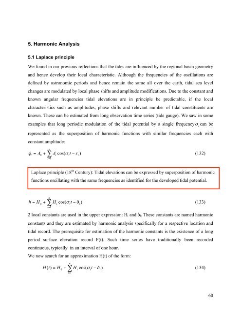
<strong>5.</strong>1 Laplace principle<br />
We found in our previous reflections that the tides are influenced by the regional basin geometry<br />
and hence develop their local characteristic. Although the frequencies of the oscillations are<br />
defined by astronomic periods and hence remain the same all over the earth, tidal sea level<br />
changes are modulated by local phase shifts and amplitude modifications. Due to the constant and<br />
known angular frequencies tidal elevations are in principle be predictable, if the local<br />
characteristics such as amplitudes, phase shifts and relevant number of tidal constituents are<br />
known. These can be estimated from long observation time series (tide gauge). We saw in some<br />
examples that long periodic modulation of the tidal potential by a single frequency can be<br />
represented as the superposition of harmonic functions with similar frequencies each with<br />
constant amplitude:<br />
(132)<br />
Laplace principle (18 th Century): Tidal elevations can be expressed by superposition of harmonic<br />
functions oscillating with the same frequencies as identified for the developed tidal potential.<br />
(133)<br />
2 local constants are used in the upper expression: Hi and δi. These constants are named harmonic<br />
constants and they are estimated by harmonic analysis specifically for a respective location and<br />
tidal record. The prerequisite for estimation of the harmonic constants is the existence of a long<br />
period surface elevation record F(t). Such time series have traditionally been recorded<br />
continuous, typically in an interval of one hour.<br />
We now search for an approximation H(t) of the form:<br />
(134)<br />
60
with defined constants Hi and δi such as H(t) best fits the observed elevation time series F(t). The<br />
number of harmonic contributions considered (n+1) specifies the degree of approximation with<br />
the upper limit being the number of harmonic contributions currently estimated (396 after<br />
Doodsen, 1921). Furthermore, the practical issue of a finite length of the observational time scale<br />
defines a limitation for the number of components to consider (and consequently for the<br />
accuracy). This is especially the case for the long periodic components in the spectra. The best fit<br />
of Hi and δi can be estimated by the least square fit method. The difference between fit and<br />
observed time series is estimated for each time step:<br />
(135)<br />
and we search for the values Hi and δi resulting in minimum values for the sum of squared<br />
differences<br />
(136)<br />
For practical purposes the time series H(t) is presented in the form:<br />
(137)<br />
We than can interpret the quadratic sum as a function of coefficients Ai and Bi and search for the<br />
minimum of G(A0,Ai,Bi ) by finding the zero of the derivatives of G with:<br />
(138)<br />
These conditions give 2n+1 equations for 2n+1 unknowns. The respective equations have the<br />
form:<br />
(139)<br />
since<br />
(140)<br />
follows<br />
(141)<br />
or in detail<br />
61
m<br />
m<br />
∑ F(t)cosσ i<br />
t = ∑[A 0<br />
+ ∑ A i<br />
cos(σ i<br />
t) + ∑ B i<br />
sinσ i<br />
t]cosσ i<br />
t<br />
t=1<br />
t=1 t=1<br />
i=1<br />
m<br />
m<br />
n<br />
n<br />
= ∑ A 0<br />
cosσ i<br />
t + ∑cosσ i<br />
t∑ A i<br />
cosσ i<br />
t + ∑cosσ i<br />
t∑B i<br />
sinσ i<br />
t<br />
i=1<br />
i=1<br />
i=1<br />
i=1<br />
i=1<br />
n<br />
m<br />
n<br />
(142)<br />
€<br />
Corresponding sets of equations are received by using the last equation of (138). m is in general a<br />
quite large number (with hourly time step already 8760 for every year), hence solving the upper<br />
equations is a huge task and a fast solver with high performance are needed. For an almost<br />
complete estimation, about 390 harmonic components are needed. To reach a high degree of<br />
accuracy about 115 semi-diurnal, 160 diurnal and 100 long periodic components are needed to be<br />
considered. Less accurate with a still sufficient degree of accuracy can be achieved using a much<br />
lower number of harmonic components.<br />
<strong>5.</strong>2 Tidal prediction with 7 components<br />
From a tidal table from a nearby observation point, we can find out the frequencies and the<br />
harmonics constants for the 7 most prominent spectral lines. If we neglect the long-periodic<br />
contributions, especially the half-year and yearly contributions, the 7 most important<br />
contributions are K2, M2, N2 and S2 (semi-diurnal) and K1, O1 and P1 (diurnal).<br />
Tidal prediction will be performed based on the same principles as used in the previous section,<br />
i.e. we apply a formulae of the type:<br />
(155)<br />
Time is thereby counting from beginning of every year, phase δ i is therefore related to a<br />
calculation of time which begins at New Year every year. The general phase δ i will be separated<br />
into two contributions, (V0+u)i and χi. (V0+u)i is the equilibrium phase of the tidal component<br />
(in the tidal potential) to the 0-meridian at New Year and χi is the epoch of the tide, the own<br />
anomaly of the tidal component from the equilibrium tidal phase. It is common praxis to further<br />
split up the epoch of a tide into a local contribution and a contribution depending on geographic<br />
length.<br />
62
Equilibrium phase can be found in standard tables, normally published for many years in<br />
advance. In the following table, you find harmonic constants for Bergen together with the<br />
equilibrium phase and epoch for 1.1.1990.<br />
Component Frequency Amplitude Epoch Vo+u<br />
K1 15,04107 3,2 cm 170 16,7<br />
O1 13,94304 3,0 cm 17 240,1<br />
P1 14,98593 1,1 cm 152 349,6<br />
K2 30,08214 4,6 cm 337 213,9<br />
S2 30 15,8 cm 335 0<br />
M2 28,98410 43,9 cm 298 259,4<br />
N2 28,43973 8,4 cm 270 324,3<br />
Using the upper table as a starting point, we are able to perform a tidal prediction for a full year.<br />
For a more precise estimation we’ll perform the analysis for a month and start every month under<br />
consideration of a new equilibrium tidal phase at the beginning of the respective month (found in<br />
additional tables).<br />
6 Appendix<br />
6.1 <strong>Harmonic</strong> analysis of short time series<br />
In case we would like to find a mathematical representation of tidal contributions from a much<br />
shorter time series, e.g. for observations of tidal currents, which in contrast to the surface<br />
elevation, are typically observed only during a short period of instruments deployment, the<br />
previous type of analysis can not be applied. Here we need another approach to receive a<br />
mathematic representation for the periodic contributions. Although surface elevation records are<br />
typically available for long time periods, limitations using the previous analysis method could<br />
arise as well in case of analysing daily variations of surface elevation. If the temporal variability<br />
of observations is related to tidal forcing, it is near by hand to introduce moon hours (to simplify)<br />
as time variable, which we’ll use in the following. We furthermore have to consider, that in<br />
63
addition to the tidal forcing from the tidal potential, real surface elevations are partly caused by<br />
resonance, which can occur on shorter time scales than 12h. Hence, we’ll find periodic<br />
oscillations with periods shorter than 12 hours. This might create a significant contribution of<br />
short periodic disturbances, which we have to account for to enable realistic prediction. We<br />
therefore need to include representation of higher harmonic components, which cannot be found<br />
from celestial periods.<br />
We assume that the observed height X(t) can be represented by the following series<br />
approximation:<br />
(143)<br />
where σ is the basic diurnal frequency with 2π/24 rad/h and t is measured in moon hours. Hence<br />
we consider diurnal and semidiurnal tidal variations and high frequency disturbances (resonance<br />
and unresolved long periodic variability). We multiply the equation with cos (nσt) and integrate<br />
over one (moon) day. As generally known, we’ll have only a contribution from the first term of<br />
the series (A n –coefficient), namely:<br />
(144)<br />
with introduction of ω=nσt (144) reduce to<br />
(145)<br />
The amplitudes A n can therefore be estimated by the following equation:<br />
(146)<br />
Accordingly we’ll find that<br />
In practice, the variable will be reported as an hour value (or discrete). Hence, we need to<br />
discretize the above form. Below we’ll find the expression for the daily basic diurnal frequency<br />
(n=1):<br />
64
(147)<br />
(148)<br />
Similarly we get the coefficients for the semi-diurnal components (n=2):<br />
(149)<br />
(150)<br />
Components of higher harmonic frequencies can be estimated in the same way.<br />
Removing of trends<br />
For the upper analysis we assumed that the observed disturbance behave periodic. In case this is<br />
not true, we’ll fail in calculating the amplitudes using the upper method. We can avoid this by<br />
correcting the observation material from irregularities. Particularly, trends have to be removed<br />
from the observations, i.e. A0 is not a constant, but varies with observation period A0= A0(t). We<br />
compensate for such trends by reconstructing a data set without such a trend but conserving the<br />
main periodic features of the time series. For the daily oscillation we’ll achieve this by:<br />
replace X0 by (X0 +X23)/2 and<br />
replace X1 by (X1+X22)/2 etc.<br />
in the cosine summation, but use the half-difference for the sine summation.<br />
Filtering<br />
In oceanography we use a series method to remove high frequency disturbances. In case of long<br />
time series, such disturbances are normally no problem and it is not necessary to apply particular<br />
methods to remove these before performing the upper analysis. However, for shorter time series,<br />
these disturbances might cause failure of the upper analysis and we need to remove them before<br />
we perform a harmonic analysis. Here we won’t discuss the more advanced methods for filtering,<br />
but introduce a simple filter, i.e. the moving averaged. This method is widely applied in<br />
oceanography and particularly used for analyzing tidal records. In dependence of the<br />
observational material which is typically available in hourly resolution, appropriate filtering of<br />
65
high frequency disturbances can be achieved by creation of an average for every hour in the<br />
form:<br />
(151)<br />
The interval used for averaging depends on the frequencies of the disturbances, but normally 4<br />
hours are sufficient. While performing filtering, we need to account for that we’ll flatten as well<br />
the tidal signal while averaging, and hence we have to compensate for this effect. The flattening<br />
of signals will be stronger for higher frequencies, i.e. compensation factors for semi-diurnal<br />
periods will be stronger than for diurnal periods.<br />
A useful 36-hours analysis method compensated for trends<br />
In case of short time series, observed only over a couple of days, we cannot hope to extract many<br />
daily or half daily or longer periodic components. Nevertheless, such a time series can be useful<br />
to study the semi-diurnal and diurnal tidal characteristics and possible longer periodic<br />
contributions, e.g. if an experiment is performed during spring and neap tide, it is possible to<br />
represent the tidal phenomena as a composite of 2 respective components. This can be achieved<br />
by using the following useful method, which uses series with at least 37 hourly values. The<br />
calculation will be repeated every 12th or 24th hours in dependence of the length of the time<br />
series. The method was developed for calculation by hand, but can be easily programmed on a<br />
PC.<br />
Starting point of calculation is the time series, i.e. the first 37 hour steps of the observed surface<br />
elevation as a 6x7 matrix Mij:<br />
X1 X7 X13 X19 X25 X31<br />
X2 X8 X14 X20 X26 X32<br />
X3 X9 X15 X21 X27 X33<br />
Mij = X4 X10 X16 X22 X28 X34<br />
X5 X11 X17 X23 X29 X35<br />
X6 X12 X18 X24 X30 X36<br />
X7 X13 X19 X25 X31 X37<br />
From this matrix we can now calculate a vector S i by multiplication<br />
Si=MijFj<br />
66
whereby Fj is a vector with the following 6 elements:<br />
Fj =(‐1, 3, ‐4, 4, ‐3, 1)<br />
Multiplication with Fj represents a way of averaging of the assumed harmonic characteristic<br />
of the variable. The resulting vector S i is a consist of weighted sums, i.e. S1 is a weighted<br />
sum with contribution of term 1, 7, 13, 19, 25 and 31. This particular weighting gives the<br />
most weight to contributions which are in the centre of the time series. S i has 7 elements,<br />
which cover a half period centred around the centre value of the time series X19.<br />
Further smoothing can be reached by pair‐wise subtraction and addition of values which<br />
are found in equidistance from centre value S4, hence:<br />
M1=S1‐S7<br />
N1=S1+S7<br />
M2=S2‐S6<br />
N2=S2+S6<br />
M3=S3‐S5<br />
N3=S3+S5<br />
M4=S4‐S4<br />
N4=2S4<br />
M‐time series will now contain the respective sinus contribution, distributed by hour time<br />
steps 3,2, 1 and 0 hours from central values X19. The respective N‐time series contains the<br />
cosine contribution.<br />
The actual harmonic analysis will be performed by defining values Y and Z by integration of<br />
the reduced Si, to be multiplicated by cos(nσt) and sin (nσt), respectively:<br />
(152)<br />
(153)<br />
The resulting heights Y and Z are both relative measures of contributions of Acos σt and Bsinσt.<br />
The respective amplitudes A and B are received by reducing:<br />
and (154)<br />
This is without a compensation for high frequency noise. It is easy to understand that the<br />
averaging from above as well removes trends from the observational material.<br />
67
6.2 <strong>Analysis</strong> of rotating tidal currents<br />
Observing the currents in a fixed location in the sea, we’ll find tidal currents with overlaid<br />
residual currents. By removing the residual current, we’ll realize that the tidal currents form a<br />
periodic rotation of current vectors together with periodic variations in the current speed, both<br />
usually not in phase. We separate such a time series by decomposition into 2 main current<br />
directions, i.e. into an eastward component u(t) and a northward component v(t).<br />
Assuming a tidal disturbance varying with the main frequency σ, which is typically semi-diurnal,<br />
we can than estimate the periodic variation in the 2 (horizontal) current components by:<br />
(156)<br />
Or using an equivalent description:<br />
(157)<br />
Instead of the 4 coefficients M,N, P and Q we use 2 amplitude coefficients and 2 phase angles α<br />
and β, with<br />
(158)<br />
We than can find that<br />
(159)<br />
and<br />
(160)<br />
Let us now discuss the combined tidal phenomena. First, we concentrate on the absolute current<br />
speed V, with<br />
(161)<br />
68
This equation tells us, that the current speed varies harmonically between 2 extremes. Maximum<br />
values will occur when<br />
(162)<br />
Hence in case of:<br />
(163)<br />
or<br />
(164)<br />
Maximum value of V is A+B.<br />
Analogous we can find the minimum values appears at<br />
(165)<br />
and hence<br />
(166)<br />
The minimum value is V=A-B.<br />
The upper equations predict also the time when the components of tidal currents are at<br />
maximum, i.e. along the large half axis. Currents are at minimum along the small half axis.<br />
Estimation of position of the half axis will be found by in the following. Direction of the current<br />
vector V(u(t),v(t)) varies in t with u(t) and v(t). Assuming the angle between the current vector<br />
and the x-axis counting positively in anticlockwise direction, we’ll find the direction of the large<br />
half axis by<br />
(167)<br />
This can be reduced to<br />
(168)<br />
The large half axis has therefore an orientation of:<br />
(169)<br />
69
Literature<br />
Cartwright, DE, Tides –A scientific history, Cambridge University Press.<br />
Gade, HG. Tidevann og tidevannstrømmer, Teori, opptreden, analyse og prediksjon, lecture notes<br />
of GEOF331, in Norwegian<br />
Gjenne, B, Simmensen, T, 1963. Tidal choking in the landlocked fjord of Norddåsvatnet. Sarsia,<br />
11, 43-73.<br />
Ippen, AT ed., 1966. Estuary and coastline hydrodynamics. McGraw-Hill Book Comp. 744 pp.<br />
Jensen, E., 1977. Tidevannet I oslofjorden, og strøm og hydrografi I Drøbaksundet juni/juli 1972.<br />
Hovedfagsoppgave I geofysikk, Univ. i Oslo.<br />
Kvinge, T, Lee, AJ, Sætre, R, 1968. Report on study of variability in the Norwegian Sea<br />
April/May 1967. Geofysik inst., Univ. i Bergen.<br />
Mcclimans, TA, 1978. On the energetics of tidal inlets to landlocked fjords. Mar. Sc. Comm. 4.<br />
121-137.<br />
Proudman, J, Doodson, AT, 1924. The principal constituent of the tides of the North Sea.<br />
Philosophical Transactions of the Royal Society of London. Series A, Containing Papers<br />
of a Mathematical or Physical Character, Vol. 224. (1924), pp. 185-219.<br />
Pugh, DE, Tides, Surges and Mean Sea Level, John Wiley & Sons.<br />
Stewart, RH, Introduction to Physical Oceanography, Department of Oceanography, Texas<br />
University.<br />
Stigebrandt, A., 1980. Some aspects of tidal interaction with fjord constructions. Est. Coast. Mar.<br />
Sc. 11, 151-166.<br />
70