Comparison for Image Edge Detection Algorithms - IOSR
Comparison for Image Edge Detection Algorithms - IOSR
Comparison for Image Edge Detection Algorithms - IOSR

You also want an ePaper? Increase the reach of your titles
YUMPU automatically turns print PDFs into web optimized ePapers that Google loves.
<strong>IOSR</strong> Journal of Computer Engineering (<strong>IOSR</strong>JCE)<br />
ISSN: 2278-0661 Volume 2, Issue 6 (July-Aug. 2012), PP 01-04<br />
www.iosrjournals.org<br />
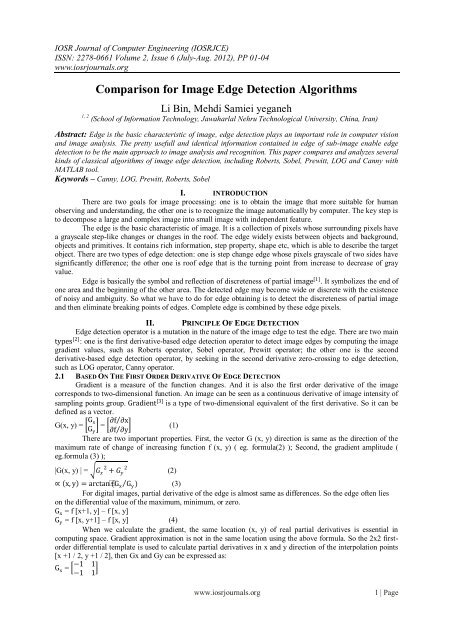
<strong>Comparison</strong> <strong>for</strong> <strong>Image</strong> <strong>Edge</strong> <strong>Detection</strong> <strong>Algorithms</strong><br />
Li Bin, Mehdi Samiei yeganeh<br />
1, 2 (School of In<strong>for</strong>mation Technology, Jawaharlal Nehru Technological University, China, Iran)<br />
Abstract: <strong>Edge</strong> is the basic characteristic of image, edge detection plays an important role in computer vision<br />
and image analysis. The pretty usefull and identical in<strong>for</strong>mation contained in edge of sub-image enable edge<br />
detection to be the main approach to image analysis and recognition. This paper compares and analyzes several<br />
kinds of classical algorithms of image edge detection, including Roberts, Sobel, Prewitt, LOG and Canny with<br />
MATLAB tool.<br />
Keywords – Canny, LOG, Prewitt, Roberts, Sobel<br />
I. INTRODUCTION<br />
There are two goals <strong>for</strong> image processing: one is to obtain the image that more suitable <strong>for</strong> human<br />
observing and understanding, the other one is to recognize the image automatically by computer. The key step is<br />
to decompose a large and complex image into small image with independent feature.<br />
The edge is the basic characteristic of image. It is a collection of pixels whose surrounding pixels have<br />
a grayscale step-like changes or changes in the roof. The edge widely exists between objects and background,<br />
objects and primitives. It contains rich in<strong>for</strong>mation, step property, shape etc, which is able to describe the target<br />
object. There are two types of edge detection: one is step change edge whose pixels grayscale of two sides have<br />
significantly difference; the other one is roof edge that is the turning point from increase to decrease of gray<br />
value.<br />
<strong>Edge</strong> is basically the symbol and reflection of discreteness of partial image [1] . It symbolizes the end of<br />
one area and the beginning of the other area. The detected edge may become wide or discrete with the existence<br />
of noisy and ambiguity. So what we have to do <strong>for</strong> edge obtaining is to detect the discreteness of partial image<br />
and then eliminate breaking points of edges. Complete edge is combined by these edge pixels.<br />
II. PRINCIPLE OF EDGE DETECTION<br />
<strong>Edge</strong> detection operator is a mutation in the nature of the image edge to test the edge. There are two main<br />
types [2] : one is the first derivative-based edge detection operator to detect image edges by computing the image<br />
gradient values, such as Roberts operator, Sobel operator, Prewitt operator; the other one is the second<br />
derivative-based edge detection operator, by seeking in the second derivative zero-crossing to edge detection,<br />
such as LOG operator, Canny operator.<br />
2.1 BASED ON THE FIRST ORDER DERIVATIVE OF EDGE DETECTION<br />
Gradient is a measure of the function changes. And it is also the first order derivative of the image<br />
corresponds to two-dimensional function. An image can be seen as a continuous derivative of image intensity of<br />
sampling points group. Gradient [3] is a type of two-dimensional equivalent of the first derivative. So it can be<br />
defined as a vector.<br />
G(x, y) = G x ∂f ∂x<br />
G<br />
= (1)<br />
y ∂f ∂y<br />
There are two important properties. First, the vector G (x, y) direction is same as the direction of the<br />
maximum rate of change of increasing function f (x, y) ( eg. <strong>for</strong>mula(2) ); Second, the gradient amplitude (<br />
eg.<strong>for</strong>mula (3) );<br />
|G(x, y) | = G x 2 + G y<br />
2<br />
(2)<br />
∝ x, y = arctan(G x G y ) (3)<br />
For digital images, partial derivative of the edge is almost same as differences. So the edge often lies<br />
on the differential value of the maximum, minimum, or zero.<br />
G x = f [x+1, y] – f [x, y]<br />
G y = f [x, y+1] – f [x, y] (4)<br />
When we calculate the gradient, the same location (x, y) of real partial derivatives is essential in<br />
computing space. Gradient approximation is not in the same location using the above <strong>for</strong>mula. So the 2x2 firstorder<br />
differential template is used to calculate partial derivatives in x and y direction of the interpolation points<br />
[x +1 / 2, y +1 / 2], then Gx and Gy can be expressed as:<br />
G x = −1 1<br />
−1 1<br />
www.iosrjournals.org<br />
1 | Page
<strong>Comparison</strong> For <strong>Image</strong> <strong>Edge</strong> <strong>Detection</strong> <strong>Algorithms</strong><br />
1 1<br />
G y =<br />
(5)<br />
−1 −1<br />
2.2 Based On The First Order Derivative Of <strong>Edge</strong> <strong>Detection</strong><br />
The first order derivative method described above uses a boundary point. This method may lead to the<br />
edge points to detect excessive data storage. Theoretically more effective way is to determine the point with<br />
maximum value in ladder and these points are to be considered as edge point.<br />
This method can detect more precise edge. The first derivative of the local maximum corresponds to<br />
the second derivative zero-crossing point. So more accurate edge points can be found by the determination of<br />
the zero crossing point of the second derivative of the image gray.<br />
Fig. 1: The image of the second derivatives<br />
III. ALGORITHMS OF EDGE DETECTION<br />
3.1 Roberts operator<br />
Roberts [4] operator is a first-order operator, which uses a partial differential operator to find the edge.<br />
It uses the approximation between the two adjacent pixels of the diagonal direction of the gradient amplitude to<br />
detect edge. In the field of 2x2 diagonal derivative, the two convolution kernels, respectively; G x = 1 0<br />
0 −1 , G y<br />
0 1<br />
= as shown in Figure 2. Roberts operator is defined as:<br />
−1 0<br />
G (x, y) = f(x, y) − f(x + 1, y + 1) 2 + f(x + 1, y) − f(x, y + 1) 2 1/2 (7)<br />
Gradient size of Roberts operator represents the edge strength of the edge and direction of the gradient<br />
and the edge are vertical. The operator edge has higher positioning accuracy, but it is easy to lose a part of the<br />
edge. The operator with a steep low-noise image corresponds best.<br />
1 0<br />
0 -1<br />
0 1<br />
-1 0<br />
Fig. 2: Roberts Operator<br />
3.2 Sobel operator<br />
Sobel operator [5] is in the <strong>for</strong>m of the filtering operator. It is used to extract the edge. Each point in the<br />
image are the two nuclear convolutions. One checks maximum response of the vertical edge, and the other one<br />
checks maximum response of the horizontal edge. The maximum valueof two convolutions will be referred as<br />
output value of the changing point. Sobel operator is easy to achieve in space, has a smoothing effect on the<br />
noise, is nearly affected by noise, can provide more accurate edge direction in<strong>for</strong>mation but it will also detect<br />
many false edges with coarse edge width.<br />
-1 -2 -1<br />
0 0 0<br />
1 2 1<br />
-1 0 1<br />
-2 0 2<br />
-1 0 1<br />
Fig. 3: Sobel Operator<br />
3.3 Prewitt operator<br />
The Prewitt operator is one type of an edge model operator. Fig. 5 shows that two convolution kernels<br />
<strong>for</strong>med Prewitt operator. Model operator is made from the ideal edge sub-image composition. Detect the image<br />
using edge model one by one, and take the maximum value of the model operator that is most similar to the<br />
detected region as the output of the operator. Both Prewitt operator and Sobel operator use the same differential<br />
and filtering operations, the only difference is that the template does not use the same image.<br />
3.4 LOG operator<br />
www.iosrjournals.org<br />
2 | Page
<strong>Comparison</strong> For <strong>Image</strong> <strong>Edge</strong> <strong>Detection</strong> <strong>Algorithms</strong><br />
LOG (Laplacian of Gaussian) operator find the optimal filter of edge detection by ratio of the signal to<br />
noise of image. Firstly, a Gaussian function is used to low-pass smoothingly filter image; then high-pass filter<br />
the Laplacian operator, according to the second derivative of zero to detect the edges. Gaussian filter function [8]<br />
is:<br />
G(x, y, ) = (9)<br />
Where letter is the standard deviation of the Gaussian filter, which determines the degree of smoothing<br />
of the image. By The low-pass filtering the image f (x, y) we can get f (x, y) * G (x, y, ) and<br />
g(x,y) = (10)<br />
Where is LOG operator.<br />
3.5 Canny operator<br />
Canny proposed three criteria of the evaluation the pros and cons of per<strong>for</strong>mance of edge detection: (1)<br />
standard of ratio of signal to noise, that is real edge detection probability is higher and non-edge points<br />
sentenced to be lower the probability of edge points, so that the output of ratio of signal to noise is maximum;<br />
(2) standard of positioning accuracy, that is there is great possibility that the detected edge points is actually in<br />
center of the edge; (3) The unilateral corresponding standard, that is the probability of multiple response in<br />
single edge is low, and false edge The response should be the maximum inhibition.<br />
Canny operator [6] is based on three criteria. The basic idea uses a Gaussian function to smooth image<br />
firstly. Then the maximum value of first derivative also corresponds to the minimum of the first derivative. In<br />
other words, both points with dramatic change of gray-scale (strong edge) and points with slight change of grayscale<br />
(weak edges) correspond to the second derivative zero-crossing point. Thus these two thresholds are used<br />
to detect strong edges and weak edges. The fact that Canny algorithm is not susceptible to noise interference<br />
enables its ability to detect true weak edges.<br />
IV. COMPARISON OF EDGE DETECTION<br />
This paper use MATLAB [7] to evaluate these algorithms by setting different thresholds.<br />
4.1 The result of Roberts operator:<br />
(a) (b) (c) (d)<br />
Fig. 4 :.( a) original image (b) threshold = 0.00 (c) threshold = 0.05 (d) threshold = 0.3<br />
4.2 The result of Sobel operator:<br />
4.3 The result of Prewitt operator:<br />
(a) (b) (c)<br />
Fig. 5: (a) threshold =0.00 (b) threshold = 0.05 (c) threshold = 0.3<br />
(a) (b) (c)<br />
Fig. 6: (a) threshold = 0.00 (b) threshold = 0.05 (c) threshold = 0.3<br />
4.4 The result of Canny operator:<br />
(a) (b) (c)<br />
Fig. 7: (a) threshold = 0.00 (b) threshold = 0.05 (c) threshold =0.3<br />
www.iosrjournals.org<br />
3 | Page
<strong>Comparison</strong> For <strong>Image</strong> <strong>Edge</strong> <strong>Detection</strong> <strong>Algorithms</strong><br />
Result analysis: figure 4, 5, 6, 7 are the result of first order derivative of edge detection, The greater the<br />
threshold is, the clearer image edge processing effect is and the more coherent the edge points are significant.<br />
However, when the threshold is over 0.3, the effective in<strong>for</strong>mation of the image edge will be lost. We can see<br />
that Canny algorithm is best among all algorithms. Because Canny can filter noise and maintain the integrity of<br />
valid in<strong>for</strong>mation. Canny operator also can ensure high positioning accuracy of the image [8] . And other<br />
operators are more sensitive to noise than Canny, and cannot be filtered.<br />
4.5 The result of LOG operator:<br />
(a) (b) (c)<br />
Fig. 8: (a) threshold = 0.00 (b) threshold =0.01 (c) threshold = 0.3<br />
Result analysis: Fig. 8 is the result of second order derivative of edge detection, the smaller the<br />
threshold is, the clearer marginal treatment effect of the image is, more coherent the edge points are significant.<br />
LOG algorithm is sensitive to noise by using the algorithm of image intensity second order derivative zero<br />
crossing point. There<strong>for</strong>e, it should do denoising be<strong>for</strong>e enhance the image.<br />
It’s very necessary to detect pseudo-edge caused by noise because detection accuracy can be improved;<br />
In order to improve noise immunity, position deviation takes place. Actual image contains noise, and noise<br />
distribution, variance, and other in<strong>for</strong>mation that are unknown to us. Smoothing filter operation to eliminate<br />
noise with high-frequency signal, but detected edge shifts.<br />
Due to factor of physical and light the edge of the actual image often has different scales, and each<br />
edge pixel scale is unknown. It’s not possible to detect edge very well by using a single fixed-scale edge<br />
detection operator.<br />
Classical edge detection methods [10] are extremely sensitive to noise due to the introduction of<br />
various <strong>for</strong>ms of differential operation. Noise is detected as edge points in edge detection instead of real edge<br />
with interference of noise. Thus a good edge detection method should have good noise immunity and<br />
outstanding property of restraining noises which are the advantages of Canny operator.<br />
V. CONCLUSION<br />
One-dimensional operator Roberts, Sobel and Prewitt are able to handle treatment effect of images of<br />
more gray-scale gradient and noise. The Sobel operator is more sensitive to the diagonal edge is than to the<br />
horizontal and vertical edges. On the contrary, Prewitt operator is more sensitive to horizontal and vertical<br />
edges.<br />
LOG often produces the edge of double pixels wide; there<strong>for</strong>e, LOG operator is rarely directly used <strong>for</strong><br />
edge detection. It is mainly used to determine pixels to determine if the pixels of image are in the dark areas or<br />
bright area of the known edge.<br />
Canny operator is based on three criteria. The basic idea uses a Gaussian function to smooth image<br />
firstly. Then the maximum value of first derivative also corresponds to the minimum of the first derivative. In<br />
other words, both points with dramatic change of gray-scale (strong edge) and points with slight change of grayscale<br />
correspond to the second derivative zero-crossing point. Thus these two thresholds are used to detect<br />
strong edges and weak edges. The fact that Canny algorithm is not susceptible to noise interference enables its<br />
ability to detect true weak edges. Canny algorithm is not susceptible to noise interference enables its ability to<br />
detect true weak edges. It’s optimal edge detection algorithm.<br />
REFERENCES<br />
Journal Papers:<br />
[1] L.P. Han and W.B. Yin. An Effective Adaptive Filter Scale Adjustment <strong>Edge</strong> <strong>Detection</strong> Method(China, Tsinghua university, 1997).<br />
[2] D. Marr and E. Hildreth, Theory of <strong>Edge</strong> <strong>Detection</strong>(London, 1980).<br />
[3] Q.H Zhang, S Gao, and T.D Bui, <strong>Edge</strong> detection models, Lecture Notes in Computer Science, 32(4), 2005, 133-140.<br />
[4] D.H Lim, Robust <strong>Edge</strong> <strong>Detection</strong> In Noisy <strong>Image</strong>s, Computational Statistics & Data Analysis, 96(3), 2006, 803-812.<br />
[5] Abbasi TA, Abbasi MU, A novel FPGA-based architecture <strong>for</strong> Sobel edge detection operator, International Journal of Electronics, 13(9),<br />
2007, 889-896.<br />
[6] Canny John, A Computational Approach to <strong>Edge</strong> <strong>Detection</strong>, IEEE Transactions on Pattern Analysis and Machine Intelligence,<br />
PAMI-8(6), 1986, 679-6987<br />
[7] X.L Xu, Application of Matlab In Digital <strong>Image</strong> Processing, Modern Computer, 43(5), 2008, 35-37.<br />
[8] Y.Q Lv and G.Y Zeng , <strong>Detection</strong> Algorithm of Picture <strong>Edge</strong>, TAIYUANSCIENCE & TECHNOLOGY, 27(2), 2009, 34-35<br />
[9] D.F Zhang, MATLAB Digital <strong>Image</strong> Processing(Beijing, Mechanical Industry, 2009)<br />
www.iosrjournals.org<br />
4 | Page