Appendix B Vector Calculus in Three Dimensions - School of ...

Appendix B
VectorCalculusinThreeDimensions
In this appendix, we review the fundamentals of three-dimensional vector calculus.
The student is expected to have already encountered most of these topics in an introductory
multi-variable calculus course. We shall be dealing with calculus on curves, surfaces
and solid bodies in three-dimensional space. The three methods of integration — line,
surface and volume (triple) integrals — and the fundamental vector differential operators
— gradient, curl and divergence — are intimately related. The differential operators and
integrals underlie the multivariate versions of the fundamental theorem of calculus, known
as Stokes’ Theorem and the Divergence Theorem.
All of these topics will be reviewed in rapid succession, with most details being relegated
to the exercises. A more detailed development can be found in any reasonable
multi-variable calculus text, including [9,46,70].
B.1. Dot and Cross Product.
We begin by reviewing the basic algebraic operations between vectors in three-dimensional
space R 3 . We shall continue to use column vector notation
v =
⎛
⎝ v ⎞
1
v 2
⎠ = (v 1 ,v 2 ,v 3 ) T ∈ R 3 .
v 3
The standard basis vectors of R 3 are
⎛ ⎞
⎛
⎞
⎛
⎞
e 1 = i =
⎝ 1 0
0
⎠, e 2 = j =
⎝ 0 1⎠, e 3 = k =
0
⎝ 0 0
1
⎠. (B.1)
We prefer the former notation, as it easily generalizes to n-dimensional space. Any vector
v =
⎛
⎝ v ⎞
1
v 2
⎠ = v 1 e 1 +v 2 e 2 +v 3 e 3
v 3
isalinearcombinationofthe basisvectors. The coefficients hev 1 ,v 2 ,v 3 arethecoordinates
of the vector with respect to the standard basis.
12/11/12 1230 c○ 2012 Peter J. Olver

Space comes equipped with an orientation — either right- or left-handed. One cannot
alter † the orientation by physical motion, although looking in a mirror — or, mathematically,
performing a reflection — reverses the orientation. The standard basis vectors are
graphed with a right-hand orientation, as in Figure rhr . When you point with your right
hand, e 1 lies in the direction of your index finger, e 2 lies in the direction of your middle
finger, and e 3 is in the direction of your thumb. In general, a set of three linearly independent
vectors v 1 ,v 2 ,v 3 is said to have a right-handed orientation if they have the same
orientation as the standard basis. It is not difficult to prove that this is the case if and
only if the determinant of the 3×3 matrix whose columns are the given vectors is positive:
det(v 1 ,v 2 ,v 3 ) > 0. Interchanging the order of the vectors may switch their orientation;
for example if v 1 ,v 2 ,v 3 are right-handed, then v 2 ,v 1 ,v 3 is left-handed.
We have already made extensive use of the Euclidean dot product
⎛ ⎛
v·w = v 1 w 1 +v 2 w 2 +v 3 w 3 , where v =
along with the Euclidean norm
⎝ v ⎞
1
v 2
v 3
⎠, w =
⎝ w ⎞
1
w 2
w 3
⎠, (B.2)
‖v‖ = √ v·v = √ v 2 1 +v2 2 +v2 3 .
(B.3)
As in Definition 3.1, the dot product is bilinear, symmetric: v ·w = w ·v, and positive.
The Cauchy–Schwarz inequality
|v·w| ≤ ‖v‖‖w‖.
(B.4)
implies that the dot product can be used to measure the angle θ between the two vectors
v and w:
v·w = ‖v‖‖w‖ cosθ.
(B.5)
(See also (3.17).)
Remark: In this chapter, we will only use the Euclidean dot product and its associated
norm. Adapting the constructions to more general norms and inner products is an
interesting exercise, but will not concern us here.
Also of great importance — but particular to three-dimensional space — is the cross
product between vectors. While the dot product produces a scalar, the three-dimensional
cross product produces a vector, defined by the formula
v×w =
⎛
⎝ v 2 w 3 −v 3 w ⎞
2
v 3 w 1 −v 1 w 3
⎠ where v =
v 1 w 2 −v 2 w 1
⎛
⎝ v ⎞
1
v 2
⎠, w =
v 3
⎛
⎝ w ⎞
1
w 2
⎠, (B.6)
w 3
† This assumes that space is identified with the three-dimensional Euclidean space R 3 , or,
more generally, an oriented three-dimensional manifold, [21].
12/11/12 1231 c○ 2012 Peter J. Olver

We have chosen to employ the more modern wedge notation rather the more traditional
cross symbol, v×w, for this quantity. The cross product formula is most easily memorized
as a formal 3×3 determinant
⎛
v×w = det⎝ v ⎞
1 w 1 e 1
v 2 w 2 e 2
⎠ = (v 2 w 3 −v 3 w 2 )e 1 +(v 3 w 1 −v 1 w 3 )e 2 +(v 1 w 2 −v 2 w 1 )e 3 ,
v 3 w 3 e 3
(B.7)
involving the standard basis vectors (B.1). We note that, like the dot product, the cross
product is a bilinear function, meaning that
(cu+dv)×w = c(u×w)+d(v×w), u×(cv+dw) = c(u×v)+d(u×w),
(B.8)
for any vectors u,v,w ∈ R 3 and any scalars c,d ∈ R. On the other hand, unlike the dot
product, the cross product is an anti-symmetric quantity
v×w = −w×v,
(B.9)
which changes its sign when the two vectors are interchanged. In particular, the cross
product of a vector with itself is automatically zero:
v×v = 0.
Geometrically, the cross product vector u = v×w is orthogonal to the two vectors v
and w:
v·(v×w) = 0 = w·(v×w).
Thus, when v and w are linearly independent, their cross product u = v×w ≠ 0 defines
a normal direction to the plane spanned by v and w. The direction of the cross product
is fixed by the requirement that v,w,u = v ×w form a right-handed triple. The length
of the cross product vector is equal to the area of the parallelogram defined by the two
vectors, which is
‖v×w‖ = ‖v‖‖w‖|sinθ|
(B.10)
where θ is than angle between the two vectors, as in Figure para . Consequently, the cross
product vector is zero, v × w = 0, if and only if the two vectors are collinear (linearly
dependent) and hence only span a line.
The scalar triple product u·(v×w) between three vectors u,v,w is defined as the
dot product between the first vector with the cross product of the second and third vectors.
The parenthesis is often omitted because there is only one way to make sense of
u·v × w. Combining (B.2), (B.7), shows that one can compute the triple product by the
determinantal formula ⎛
u·v×w = det⎝ u ⎞
1 v 1 w 1
u 2 v 2 w 2
⎠. (B.11)
u 3 v 3 w 3
By the properties of the determinant, permuting the order of the vectors merely changes
the sign of the triple product:
u·v×w = −v·u×w = +v·w×u = ··· .
12/11/12 1232 c○ 2012 Peter J. Olver

The triple product vanishes, u · v × w = 0, if and only if the three vectors are linearly
dependent, i.e., coplanar or collinear. The triple product is positive, u·v×w > 0 if and
only if the three vectors form a right-handed basis. Its magnitude |u·v×w| measures
the volume of the parallelepiped spanned by the three vectors u,v,w, as in Figure ppp .
B.2. Curves.
A space curve C ⊂ R 3 is parametrized by a vector-valued function
⎛
x(t) = ⎝ x(t)
⎞
y(t) ⎠ ∈ R 3 , a ≤ t ≤ b, (B.12)
z(t)
that depends upon a single parameter t that varies over some interval. We shall always
assume that x(t) is continuously differentiable. The curve is smooth provided its tangent
vector is continuous and everywhere nonzero:
⎛ ⎞
x
dx
dt = x = ⎝ yz ⎠ ≠ 0.
(B.13)
As in the planar situation, the smoothness condition (B.13) precludes the formulation of
corners, cusps or other singularities in the curve.
Physically, we can think of a curve as the trajectory described by a particle moving in
space. At each time t, the tangent vector x(t) represents the instantaneous velocity of the
particle. Thus, as long as the particle moves with nonzero speed, ‖ x‖ = √
x 2 + y 2 + z 2 >
0, its trajectory is necessarily a smooth curve.
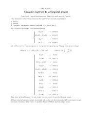
Example B.1. Acharged particleinaconstant magneticfield movesalongthecurve
⎛
x(t) = ⎝ ρ cost
⎞
ρ sint⎠, (B.14)
ct
where c > 0 and ρ > 0 are positive constants. The curve describes a circular helix of radius
ρ spiraling up the z axis. The parameter c determines the pitch of the helix, indicating
how tightly its coils are wound; the smaller c is, the closer the winding. See Figure B.1 for
an illustration. DNA is, remarkably, formed in the shape of a (bent and twisted) double
helix. The tangent to the helix at a point x(t) is the vector
x(t) =
⎛
⎝
−ρ sint
ρ cost
c
Note that the speed of the particle,
√
‖ x‖ = ρ 2 sin 2 t+ρ 2 cos 2 t+c 2 = √ ρ 2 +c 2 ,
remains constant, although the velocity vector x twists around.
⎞
⎠.
(B.15)
12/11/12 1233 c○ 2012 Peter J. Olver

-0.5
-1
-1 -0.5 0.5 1 0 0.5 0
1
10
0
-10
Figure B.1.
A Helix.
Most of the terminology introduced in Chapter A for planar curves carries over to
space curves without significant alteration. In particular, a curve is simple if it never
crosses itself, and closed if its ends meet, x(a) = x(b). In the plane, simple closed curves
are all topologically equivalent, meaning one can be continuously deformed to the other.
In space, this is no longer true. Closed curves can be knotted, and thus have nontrivial
topology.
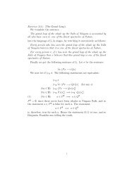
Example B.2. The curve
⎛
x(t) = ⎝ (2+cos3t)cos2t
⎞
(2+cos3t)sin2t⎠ for 0 ≤ t ≤ 2π, (B.16)
sin3t
describes a closedcurve that isintheshape of a trefoilknot, asdepicted inFigureB.2. The
trefoil is a genuine knot, meaning it cannot be deformed into an unknotted circle without
cutting and retying. (However, a rigorous proof of this fact is not easy.) The trefoil is the
simplest of the “toroidal knots”, investigated in more detail in Exercise B.2.6.
The study and classification of knots is a subject of great historical importance. Indeed,
they were first considered from a mathematical viewpoint in the nineteenth century,
when the English applied mathematician William Thompson (later Lord Kelvin) proposed
a theory of atoms based on knots! In recent years, knot theory has witnessed a tremendous
revival, owing to its great relevance to modern day mathematics and physics. We refer the
12/11/12 1234 c○ 2012 Peter J. Olver

Figure B.2.
Two Views of a Trefoil Knot.
interested reader to the advanced text [115] for details.
B.3. Line Integrals.
In Section A.5, we encountered three different types of line integrals along plane
curves. Two of these — integrals with respect to arc length, (A.35), and circulation
integrals, (A.37) — are directly applicable to space curves. On the other hand, for threedimensional
flows, the analog of the flux line integral (A.42) is a surface integral, and will
be discussed later in the chapter.
Arc Length
The length of the space curve x(t) over the parameter range a ≤ t ≤ b is computed
by integrating the norm of its tangent vector:
∫ b
∫ L(C) =
dx
b
∥ dt ∥ dt = √ x 2 + y 2 + z 2 dt. (B.17)
a
It is not hard to show that the length of the curve is independent of the parametrization
— as it should be.
Starting at the endpoint x(a), the arc length parameter s is given by
s =
∫ t
a
∥
dx
dt
a
∥ dt and so ds = ‖ x‖dt = √
x 2 + y 2 + z 2 dt. (B.18)
The arc length s measures the distance along the curve starting from the initial point x(a).
Thus, the length of the part of the curve between s = α and s = β is exactly β − α. It
is often convenient to reparametrize the curve by its arc length, x(s). This has the same
effect as moving along the curve at unit speed, since, by the chain rule,
dx
ds = dx
dt
∥
dt x ∥∥∥
ds = ‖ x‖ , so that dx
ds
∥ = 1.
12/11/12 1235 c○ 2012 Peter J. Olver

Therefore dx/ds is the unit tangent vector pointing in the direction of motion along the
curve.
Example B.3. The length of one turn of a helix (B.14) is, using (B.15),
∫ 2π
∫ L(C) =
dx
2π
∥ dt ∥ dt = √
ρ2 +c 2 dt = 2π √ ρ 2 +c 2 .
0
0
The arc length parameter, measured from the point x(0) = (r,0,0) T is merely a rescaling,
s =
∫ t
0
√
ρ2 +c 2 dt = √ ρ 2 +c 2 t,
of the original parameter t. When the helix is parametrized by arc length,
(
) T
s
x(s) = ρ cos √
ρ2 +c , ρ sin s
√ 2 ρ2 +c , cs
√ ,
2 ρ2 +c 2
we move along it with unit speed. It now takes time s = 2π √ ρ 2 +c 2 to complete on turn
of the helix.
Example B.4. To compute the length of the trefoil knot (B.16), we begin by computing
the tangent vector
⎛
⎞
−2(2+cos3t)sin2t−3 sin3t cos2t
dx
dt = ⎝ 2(2+cos3t)cos2t−3 sin3t sin2t ⎠.
3 cos3t
After some algebra involving trigonometric identities, we find
‖ x‖ = √ 27+16 cos3t+2 cos6t ,
which is never 0. Unfortunately, the resulting arc length integral
∫ 2π
0
‖ x‖dt =
∫ 2π
0
√
27+16 cos3t+2 cos6t dt
cannot be completed in elementary terms. Numerical integration can be used to find the
approximate value 31.8986 for the length of the knot.
The arc length integral of a scalar field u(x) = u(x,y,z) along a curve C is
∫ ∫ l ∫ l
uds = u(x(s))ds = u(x(s),y(s),z(s))ds,
C
0
0
(B.19)
where l is the total length of the curve. For example, if ρ(x,y,z) represents ∫ the density at
position x = (x,y,z) of a wire bent in the shape of the curve C, then ρds represents
the total mass of the wire. In particular, the integral
∫ ∫ l
ds = ds = l
C
12/11/12 1236 c○ 2012 Peter J. Olver
0
C

ecovers the length of the curve.
If it isnot convenient to work directly with the arc length parametrization, we can still
compute the arc length integral in terms of the original parametrization x(t) for a ≤ t ≤ b.
Using the change of parameter formula (B.18), we find
∫ ∫ b ∫ b
uds = u(x(t)) ‖ x‖dt = u(x(t),y(t),z(t)) √
x 2 + y 2 + z 2 dt. (B.20)
C
a
a
Example B.5. The density of a wire that is wound in the shape of a helix is
proportional to its height. Let us compute the mass of one full turn of the helical wire.
Thus, the density is given by ρ(x,y,z) = az, where a is the constant of proportionality,
and we are assuming z ≥ 0. Substituting into (B.20), the total mass of the wire is
∫ ∫ 2π
L(C) = azds = act √ r 2 +c 2 dt = 2π 2 ac √ r 2 +c 2 .
Line Integrals of Vector Fields
C
0
As in the two-dimensional situation (A.37), the line integral of a vector field v along a
parametrized curve x(t) isobtained by integrationofitstangential component withrespect
to the arc length. The tangential component of v is given by
v·t, where t = dx
ds
is the unit tangent vector to the curve. Thus, the line integral of v is written as
∫ ∫
∫
v·dx = v 1 (x,y,z)dx+v 2 (x,y,z)dy+v 3 (x,y,z)dz = v·t ds.
C
C
C
(B.21)
We can evaluate the line integral in terms of an arbitrary parametrization of the curve by
the general formula
∫
C
v·dx =
=
∫ b
a
∫ b
a
v(x(t))· dx
dt dt
[
v 1 (x(t),y(t),z(t)) dx
dt +v dy
2 (x(t),y(t),z(t))
dt +v dz
3 (x(t),y(t),z(t))
dt
(B.22)
]
dt.
C
Line integrals in three dimensions enjoy all of the properties of their two-dimensional
siblings: Reversing the direction of parameterization along the curve changes the sign;
also, the integral can be decomposed into sums over components:
∫ ∫ ∫ ∫ ∫
v·dx = − v·dx, v·dx = v·dx + v·dx, C = C 1 ∪C 2 .
−C C C C 1 C 2
(B.23)
If f(x) ∫ represents a force field, e.g., gravity, electromagnetic force, etc., then its line
integral f ·dx represents the work done by moving along the curve. As in two dimensions,
work is independent of the parametrization of the curve, i.e., the particle’s speed of
traversal.
12/11/12 1237 c○ 2012 Peter J. Olver

Example B.6. Our goal is to move a mass through the force field f = (y,−x,1) T
startingfromtheinitialpoint(1,0,1) T andmovingverticallytothefinalpoint(1,0,2π) T .
Question: does it require more work to move in a straight line x(t) = (1,0,t) T or along
the spiral helix x(t) = (cost,sint,t) T , where, in both cases, 0 ≤ t ≤ 2π? The work line
integral has the form
∫ ∫ ∫ 2π
[
f ·dx = ydx−xdy +dz = y dx dy
−x
dt dt + dz ]
dt.
dt
C
Along the straight line, the amount of work is
∫
f ·dx =
As for the spiral helix,
∫
C
C
f ·dx =
C
∫ 2π
0
∫ 2π
0
0
dt = 2π.
[
− sin 2 t−cos 2 t+1 ] dt = 0.
Thus, although we travel a more roundabout route, it takes no work to move along the
helix!
Thereasonforthesecondresultisthattheforcevectorfieldf iseverywhereorthogonal
to the tangent to the curve: f ·t = 0, and so there is no tangential force exerted upon the
motion. In such cases, the work line integral
∫ ∫
f ·dx = f ·t ds = 0
C
automatically vanishes. In other words, it takes no work whatsoever to move in any
direction which is orthogonal to the given force vector.
B.4. Surfaces.
Curves are one-dimensional, and so can be traced out by a single parameter. Surfaces
are two-dimensional, and hence require two distinct parameters. Thus, a surface S ⊂ R 3
is parametrized by a vector-valued function
x(p,q) = (x(p,q),y(p,q),z(p,q)) T
C
(B.24)
that depends on two variables. As the parameters (p,q) ∈ Ω range over a prescribed
plane domain Ω ⊂ R 2 , the locus of points x(p,q) traces out the surface in space. See
Figure surf for an illustration. The parameters are often thought of as defining a system
of local coordinates on the curved surface.
We shall always assume that the surface is simple, meaning that it does not intersect
itself, so x(p,q) = x(˜p,˜q) if and only if p = ˜p and q = ˜q. In practice, this condition can be
quite hard to check! The boundary
∂S = {x(p,q) | (p,q) ∈ ∂Ω}
(B.25)
of a simple surface consists of one or more simple curves, as in Figure surf . If the
underlying parameter domain Ω is bounded and simply connected, then ∂Ω is a simple
closed plane curve, and so ∂S is also a simple closed curve.
12/11/12 1238 c○ 2012 Peter J. Olver

Example B.7. The simplest instance of a surface is a graph of a function. The
parameters are the x,y coordinates, and the surface coincides with the portion of the
graph of the function z = u(x,y) that lies over a fixed domain (x,y) ∈ Ω ⊂ R 2 , as
illustrated in Figure gsurf . Thus, a graphical surface has the parametric form
x(p,q) = (p,q,u(p,q)) T , (p,q) ∈ Ω.
Thus, theparametrizationidentifies x = pand y = q, whilez = u(p,q) = u(x,y)represents
the height of the surface above the point (x,y) ∈ Ω.
For example, the upper hemisphere S + r of radius r centered at the origin can be
parametrized as a graph
z = √ r 2 −x 2 −y 2 , x 2 +y 2 < r 2 , (B.26)
sitting over the disk D r = {x 2 +y 2 < r 2 } of radius r. The boundary of the hemisphere
is the image of the circle C r = ∂D r = {x 2 +y 2 = r 2 } of radius r, and is itself a circle of
radius r sitting in the x,y plane: ∂S + r = {x2 +y 2 = r,z = 0}.
Remark: One can interpret the Dirichlet problem (15.1), (15.4) for the two-dimensional
Laplace equation as the problem of finding a surface S that is the graph of a
harmonic function with a prescribed boundary ∂S = {z = h(x,y) for (x,y) ∈ ∂Ω}.
Example B.8. Asphere S r ofradiusrcanbeexplicitlyparametrizedby twoangular
variables ϕ,θ in the form
x(ϕ,θ) = (rsinϕcosθ,rsinϕsinθ,rcosϕ), 0 ≤ θ < 2π, 0 ≤ ϕ ≤ π. (B.27)
The reader can easily check that ‖x‖ 2 = r 2 , as it should be. As illustrated in Figure
sangle , θ measures the azimuthal angle or longitude, while ϕ measures the zenith
angle or latitude. Thus, the upper hemisphere S r + is obtained by restricting the zenith
parameter to the range 0 ≤ ϕ ≤ 1 π. Each parameter value ϕ,θ corresponds to a unique
2
point on the sphere, except when ϕ = 0 or π. All points (θ,0)are mapped to the north pole
(0,0,r), while all points (θ,π) are mapped to the south pole (0,0,−r). Away from the
poles, the spherical angles provide bona fide coordinates on the sphere. Fortunately, the
polar singularities do not interfere with the overall smoothness of the sphere. Nevertheless,
one must always be careful at or near these two distinguished points.
Remark: In terrestrial cartography and navigation, the latitude is measured from the
equator, and equals 1 π−ϕ, with postive values referring to the northern hemishpere and
2
negative the southern henisphere (or, vice versa, if you are an anitpodean). The longitude
istaken withrespect to the prime meridian, throughGreenwich, England, and equalsπ−θ,
with positive vlaues referring to the western hemisphere. Of course, in practice, both are
measured in degrees rather than radians. The curves {ϕ = c} where the zenith angle takes
a prescribed constant value are the circular parallels of constant latitude — except for the
north andsouth poles which aremerely points. The equatoris atϕ = 1 π, whilethe tropics
2
of Cancer and Capricorn are 232◦ 1 ≈ 0.41 radians above and below the equator. The curves
{θ = c} where the meridial angle is constant are the semi-circular meridians of constant
longitude stretching from north to south pole. Note that θ = 0 and θ = 2π describe the
same meridian. In terrestrial navigation, latitude is the angle, in degrees, measured from
the equator, while longitude is the angle measured from the Greenwich meridian.
12/11/12 1239 c○ 2012 Peter J. Olver

Example B.9. A torus is a surface of the form of an inner tube. One convenient
parametrization of a particular toroidal surface is
x(ψ,θ) = ((2+cosψ)cosθ,(2+cosψ)sinθ,sinψ) T for 0 ≤ ψ,θ ≤ 2π. (B.28)
Note that the parametrization is 2π periodic in both ψ and θ. If we introduce cylindrical
coordinates
x = r cosθ, y = r sinθ, z,
then the torus is parametrized by
r = 2+cosψ,
z = sinψ.
Therefore, the relevant values of (r,z) all lie on the circle
(r −2) 2 +z 2 = 1 (B.29)
of radius 1 centered at (2,0). As the polar angle θ increases from 0 to 2π, the circle rotates
around the z axis, and thereby sweeps out the torus.
Remark: The sphere and the torus are examples of closed surfaces. The requirements
for a surface to be closed are that it be simple and bounded, and, moreover, have no
boundary. In general, a subset S ⊂ R 3 is bounded provided it does not stretch off infinitely
far away. More precisely, boundedness is equivalent to the existence of a fixed number
R > 0 which bounds the norm ‖x‖ < R of all points x ∈ S.
Tangents to Surfaces
Consider a surface S parameterized by x(p,q) where (p,q) ∈ Ω. Each parametrized
curve(p(t),q(t))intheparameter domainΩwillbemappedtoaparametrizedcurveC ⊂ S
contained in the surface. The curve C is parametrized by the composite map
The tangent vector
x(t) = x(p(t),q(t)) = (x(p(t),q(t)),y(p(t),q(t)),z(p(t),q(t))) T .
dx
dt = ∂x
∂p
dp
dt + ∂x
∂q
dq
dt
(B.30)
to such a curve will be tangent to the surface. The set of all possible tangent vectors to
curves passing through a given point in the surface traces out the tangent plane to the
surface at that point, as in Figure tp . Note that the tangent vector (B.30) is a linear
combination of the two basis tangent vectors
x p = ∂x ( ∂x
∂p = ∂p , ∂y
∂p , ∂z ) T
, x
∂p q = ∂x ( ∂x
∂q = ∂q , ∂y
∂q , ∂z ) T
, (B.31)
∂q
which therefore span the tangent plane to the surface at the point x(p,q) ∈ S. The first
basis vector is tangent to the curves where q = constant, while the second is tangent to
the curves where p = constant.
12/11/12 1240 c○ 2012 Peter J. Olver

Example B.10. Consider the torus T parametrized as in (B.28). The basis tangent
vectors are
⎛
∂x
∂ψ = ⎝ −(2+cosθ)sinψ
⎞ ⎛
∂x
⎠,
∂θ = ⎝
(2+cosθ)cosψ
0
⎞
−sinθ cosψ
−sinθ sinψ ⎠. (B.32)
cosθ
They serve to span the tangent plane to the torus at the point x(θ,ψ). For example, at
the point x(0,0) = (3,0,0) T corresponding to the particular parameter values θ = ψ = 0,
the basis tangent vectors are
x ψ (0,0) = (0,3,0) T = 3e 2 , x θ (0,0) = (0,0,1) T = e 3 ,
andsothetangentplaneatthisparticularpointisthe(y,z)–planespanned bythestandard
basis vectors e 2 ,e 3 .
The tangent to any curve contained within the torus at the given point will be a linear
combination of these two vectors. For instance, the toroidal knot (B.16) corresponds to
the straight line
ψ(t) = 2t, 0 ≤ t ≤ 2π, θ(t) = 3t,
in the parameter space. Its tangent vector
⎛
−(4+2cos3t)sin2t−3 sin3t cos2t
dx
dt = ⎝ (4+2cos3t)cos2t−3 sin3t sin2t
3 cos3t
lies in the tangent plane to the torus at each point. In particular, at t = 0, the knot passes
through the point x(0,0) = (3,0,0) T , and has tangent vector
⎛
dx
dt = ⎝ 0 ⎞
6⎠ dψ
= 2x ψ (0,0)+3x θ (0,0) since
dt = 2, dθ
dt = 3.
3
A point x(p,q) ∈ S on the surface is said to be nonsingular provided the basis tangent
vectors x p (p,q),x q (p,q) arelinearly independent. Thus the point is nonsingular ifand only
if the tangent vectors span a full two-dimensional subspace of R 3 — the tangent plane to
the surface at the point. Nonsingularity ensures the smoothness of the surface at each
point, which is a consequence of the general Implicit Function Theorem, [159]. Singular
points, where the tangent vectors are linearly dependent, can take the form of corners,
cusps and folds in the surface. From now on, we shall always assume that our surface is
nonsingular meaning every point is a nonsingular point.
Linear independence of the tangent vectors is equivalent to the requirement that their
cross product is a nonzero vector:
N = ∂x
∂p × ∂x ( ∂(y,z)
∂q = ∂(p,q) , ∂(z,x)
∂(p,q) , ∂(x,y) ) T
≠ 0. (B.33)
∂(p,q)
12/11/12 1241 c○ 2012 Peter J. Olver
⎞
⎠

In this formula, we have adopted the standard notation
( )
∂(x,y)
∂(p,q) = det xp x q
= ∂x
y p y q ∂p
∂y
∂q − ∂x
∂q
∂y
∂p
(B.34)
for the Jacobian determinant of the functions x,y with respect to the variables p,q, which
we already encountered in the change of variables formula (A.52) for double integrals.
The cross-product vector N in (B.33) is orthogonal to both tangent vectors, and hence
orthogonal to the entire tangent plane. Therefore, N defines a normal vector to the surface
at the given (nonsingular) point.
Example B.11. Consider a surface S parametrized as the graph of a function z =
u(x,y), and so, as in Example B.7
x(x,y) = (x,y,u(x,y)) T , (x,y) ∈ Ω.
The tangent vectors
(
∂x
∂x = 1,0, ∂u ) T
,
∂x
(
∂x
∂y = 0,1, ∂u ) T
,
∂y
span the tangent plane sitting at the point (x,y,u(x,y) on S. The normal vector is
N = ∂x
∂x × ∂x (
∂y = − ∂u ) T
∂u
,−
∂x ∂y ,1 ,
and points upwards, as in Figure graphN . Note that every point on the graph is nonsingular.
The unit normal to the surface at the point is a unit vector orthogonal to the tangent
plane, and hence given by
n = N
‖N‖ = x p ×x q
‖x p ×x q ‖ .
(B.35)
In general, the direction of the normal vector N depends upon the order of the two parameters
p,q. Computing the cross product in the reverse order, x q ×x p = −N, reverses the
sign of the normal vector, and hence switches its direction. Thus, there are two possible
unit normals to the surface at each point, namely n and −n. For a closed surface, one
normal points outwards and one points inwards.
When possible, a consistent (meaning continuously varying) choice of a unit normal
serves to define an orientation of the surface. All closed surfaces, and most other surfaces
can be oriented. The usual convention for closed surfaces is to choose the orientation
defined by the outward normal. The simplest example of a non-orientable surface is the
Möbius strip obtained by gluing together the ends of a twisted strip of paper; see Exercise
.
12/11/12 1242 c○ 2012 Peter J. Olver

Example B.12. For the sphere of radius r parametrized by the spherical angles as
in (B.27), the tangent vectors are
⎛
∂x
∂ϕ = ⎝ rcosϕcosθ
⎞ ⎛
∂x
⎠,
∂θ = ⎝ −rsinϕsinθ
⎞
⎠.
rsinϕcosθ
−r sinϕ
rsinϕcosθ
0
These vectors are tangent to, respectively, the meridians of constant longitude, and the
parallels of constant latitude. The normal vector is
⎛
N = ∂x
∂ϕ × ∂x
∂θ = ⎝ r2 sin 2 ⎞
ϕcosθ
r 2 sin 2 ϕsinθ ⎠ = rsinϕ x. (B.36)
r 2 cosϕsinϕ
Thus N is a non-zero multiple of the radial vector x, except at the north or south poles
when ϕ = 0 or π. This reconfirms our earlier observation that the poles are problematic
points for the spherical angle parametrization. The unit normal
n = N
‖N‖ = x r
determined by the spherical coordinates ϕ,θ is the outward pointing normal. Reversing
the order of the angles, θ,ϕ, would lead to the outwards normal −n = −x/r.
Remark: As we already saw in the example of the hemisphere, a given surface can be
parametrized in many different ways. In general, to change parameters
p = g(˜p,˜q),
q = h(˜p,˜q),
requires a smooth, invertible map between the two parameter domains ˜Ω → Ω. Many
interesting surfaces, particularly closed surfaces, cannot be parametrized in a single consistent
manner that satisfies the smoothness constraint (B.33) on the entire surface. In
such cases, one must assemble the surface out of pieces, each parametrized in the proper
manner. The key problem in cartography is to find convenient parametrizations of the
globe that do not significantly distort the geographical features of the planet.
A surface is piecewise smooth if it can be constructed by gluing together a finite
number of smooth parts, joined along piecewise smooth curves. For example, a cube is
a piecewise smooth surface, consisting of squares joined along straight line segments. We
shall rely on the reader’s intuition to formalize these ideas, leaving a rigorous development
to a more comprehensive treatment of surface geometry, e.g., [60].
B.5. Surface Integrals.
As with spatial line integrals, there are two important types of surface integral. The
first is the integration of a scalar field with respect to surface area. A typical application
is to compute the area of a curved surface or the mass and center of mass of a curved shell
of possibly variable density. The second type is the surface integral that computes the flux
12/11/12 1243 c○ 2012 Peter J. Olver

associated with a vector field through an oriented surface. Applications appear in fluid
mechanics, electromagnetism, thermodynamics, gravitation, and many other fields.
Surface Area
According to (B.10), the length of the cross product of two vectors measures the area
of the parallelogram they span. This observation underlies the proof that the length of the
normal vector to a surface (B.35), namely
‖N‖ = ‖x p ×x q ‖,
is a measure of the infinitesimal element of surface area, denoted
dS = ‖N‖dpdq = ‖x p ×x q ‖dpdq.
(B.37)
The total area of the surface is found by summing up these infinitesimal contributions,
and is therefore given by the double integral
∫∫ ∫∫
area S = dS = ‖x p ×x q ‖dpdq
S Ω
√
∫∫ (∂(y,z) ) 2 ( ) 2 ( ) 2
(B.38)
∂(z,x) ∂(x,y)
= + + dpdq.
∂(p,q) ∂(p,q) ∂(p,q)
Ω
The surface’s area does not depend upon the parametrizationused to compute the integral.
In particular, if the surface is parametrized by x,y as the graph z = u(x,y) of a function
over a domain (x,y) ∈ Ω, then the surface area integral reduces to the familiar form
∫∫
area S =
S
∫∫
dS =
Ω
√
1+
( ) 2 ∂u
+
∂x
( ) ∂u
∂y
A detailed justification of these formulae can be found in [9,70].
dxdy.
(B.39)
Example B.13. The well-known formula for the surface area of a sphere is a simple
consequence of the integral formula (B.38). Using the parametrization by spherical angles
(B.27) and the formula (B.36) for the normal, we find
∫∫ ∫ 2π ∫ π
area S r = dS = r 2 sinϕ dϕdθ = 4πr 2 . (B.40)
S r 0 0
Fortunately, the problematic poles do not cause any difficulty in the computation, since
they contribute nothing to the surface area integral.
Alternatively, we can compute the area of one hemisphere S r + by realizing it as a
graph
z = √ r 2 −x 2 −y 2 for x 2 +y 2 ≤ 1,
over the disk of radius r, and so, by (B.39),
∫∫
√
area S r + = x
1+
2
Ω r 2 −x 2 −y + y 2
2 r 2 −x 2 −y dxdy 2
∫∫
∫
r
r ∫ 2π
= √
r2 −x 2 −y dxdy = rρ
√ 2 r2 −ρ dθdρ = 2 2πr2 ,
Ω
12/11/12 1244 c○ 2012 Peter J. Olver
0
0

where we used polar coordinates x = ρ cosθ,y = ρ sinθ to evaluate the final integral. The
area of the entire sphere is twice the area of the hemisphere.
Example B.14. Similarly, to compute the surface area of the torus T parametrized
in (B.28), we use the tangent vectors in (B.32) to compute the normal to the torus:
⎛
N = x ψ ×x θ = ⎝ (2+cosψ)cosψcosθ
⎞
(2+cosψ)cosψsinθ ⎠, with ‖x ψ ×x θ ‖ = 2+cosψ.
(2+cosψ)sinψ
Therefore,
area T =
∫ 2π ∫ 2π
0
0
(2+cosψ)dψdθ = 8π 2 .
If S ⊂ R 3 is a surface with finite area, the mean or average of a scalar function
f(x,y,z) over S is given by
M S [f ] = 1 ∫∫
f dS.
(B.41)
area S S
For example, the mean of a function over a sphere S r = {‖x‖ = r} of radius r is explicitly
given by
M Sr
[f ] = 1
4πr 2 ∫∫‖x‖=r
f(x)dS = 1
4π
∫ 2π ∫ π
0
0
F(r,ϕ,θ)sinϕdϕdθ,
(B.42)
where F(r,ϕ,θ) is the spherical coordinate expression for the scalar function f. As usual,
the mean lies between the maximum and minimum values of the function on the surface:
min
S
f ≤ M S [f ] ≤ max
S f.
In particular, the center of mass C of a surface (assuming it has constant density) is equal
to the mean of the coordinate functions x = (x,y,z) T , so
C = (M S [x],M S [y],M S [z]) T = 1 (∫∫ ∫∫ ∫∫ T
xdS, ydS, zdS)
. (B.43)
area S S S S
More generally, the integral of a scalar field u(x,y,z) over the surface is given by
∫∫ ∫∫
udS = u(x(p,q),y(p,q),z(p,q))‖x p ×x q ‖dpdq. (B.44)
S
Ω
If S represents a thin curved shell, and u = ρ(x) the density of the material at position
x ∈ S, then the surface integral (B.44) represents the total mass of the shell. For example,
the integral of u(x,y,z) over a hemisphere S r + of radius r can be evaluated by either of
the formulae
∫∫ ∫ 2π ∫ π/2
udS = u(rcosθsinϕ,rsinθsinϕ,rcosϕ) r 2 sinϕ dϕdθ
S + r
0
∫∫
=
0
x 2 +y 2 ≤r 2
r
√
r2 −x 2 −y 2 u(x,y,√ r 2 −x 2 −y 2 ) dxdy,
(B.45)
12/11/12 1245 c○ 2012 Peter J. Olver

depending upon whether one prefers spherical or graphical coordinates.
Flux Integrals
Now assumethat S isanoriented surface withchosen unit normaln. Ifv = (u,v,w) T
is a vector field, then the surface integral
⎛
∫∫ ∫∫
∫∫
( )
v·n dS = v·xp ×x q dpdq = det⎝ u x ⎞
p x q
v y p y q
⎠dpdq (B.46)
S Ω
Ω
w z p z q
of the normal component of v over the entire surface measures its flux through the surface.
An alternative common notation for the flux integral is
∫∫
S
∫∫
v·n dS =
∫∫
=
S
Ω
udydz +vdzdx+wdxdy
(B.47)
(
u(x,y,z) ∂(y,z)
)
∂(z,x) ∂(x,y)
+v(x,y,z) +w(x,y,z) dxdy,
∂(p,q) ∂(p,q) ∂(p,q)
Note how the Jacobian determinant notation (B.34) seamlessly interacts with the integration.
In particular, if the surface is the graph of a function z = h(x,y), then the surface
integral reduces to the particularly simple form
∫∫ ∫∫ (
v·n dS = u(x,y,z) ∂z
)
∂z
+v(x,y,z)
∂x ∂y +w(x,y,z) dpdq (B.48)
S
Ω
The flux surface integral relies upon the consistent choice of an orientation or unit
normal on the surface. Thus, flux only makes sense through an oriented surface — it
doesn’t make sense to speak of “flux through a Möbius band”. If we switch normals,
using, say, the inward instead of the outward normal, then the surface integral changes
sign — just like a line integral if we reverse the orientation of a curve. Similarly, if we
decompose a surface into the union of two or more parts, with only their boundaries in
common, then the surface integral similarly decomposes into a sum of surface integrals.
Thus,
∫∫ ∫∫
v·n dS = − v·n dS,
−S
S
∫∫ ∫∫ ∫∫
(B.49)
v·n dS = v·n dS + v·n dS, S = S 1 ∪S 2 .
S 1 S 2
S
In the first formula, −S denotes the surface S with the reverse orientation. In the second
formula, S 1 and S 2 are only allowed to intersect along their boundaries; moreover, they
must be oriented in the same manner as S, i.e., have the same unit normal direction.
Example B.15. Let S denote the triangular surface given by that portion of the
plane x + y + z = 1 that lies inside the positive orthant {x ≥ 0, y ≥ 0, z ≥ 0}, as in
12/11/12 1246 c○ 2012 Peter J. Olver

Figure tri3 . The flux of the vector field v = (y,xz,0) T through S equals the surface
integral
∫∫
ydydz +xzdzdx,
S
where we orient S by choosing the upwards pointing normal. To compute, we note that
S can be identified as the graph of the function z = 1 − x − y lying over the triangle
T = {0 ≤ x ≤ 1,0 ≤ y ≤ 1−x}. Therefore, by (B.47),
∫∫
S
∫∫
ydydz +xzdzdx =
=
∫ 1 ∫ 1−x
0
0
(1−x)(y +x)dydx =
T
[
y ∂(y,1−x−y)
∂(x,y)
∫ 1
0
+x(1−x−y) ∂(1−x−y,x)
∂(x,y)
( 1
2 + 1 2 x− 1 2 x2 + 1 2 x3) dx = 17
24 .
]
dxdy
If v represents the velocity vector field for a steady state fluid flow, then its flux
integral (B.46) tells us the total volume of fluid passing through S per unit time. Indeed,
at each point on S, the volume fluid that flows across a small part the surface in unit time
will fill a thin cylinder whose base is the surface area element dS and whose height v ·n
is the normal component of the fluid velocity v, as pictured in Figure fluxs . Summing
(integrating)allthesefluxcylindervolumesoverthesurfaceresultsinthefluxintegral. The
choice of orientation or unit normal specifies the convention for measuring the direction of
positive flux through the surface. If S is a closed surface, and we choose n to be the unit
outward normal, then the flux integral (B.46) represents the net amount of fluid flowing
out of the solid region bounded by S per unit time.
Example B.16. The vector field v = (0,0,1) T represents a fluid moving with constant
velocity in the vertical direction. Let us compute the fluid flux through a hemisphere
S r
{z + = = √ ∣ } ∣∣
r 2 −x 2 −y 2 x 2 +y 2 ≤ 1 ,
sitting over the disk D r of radius r in the x,y plane. The flux integral over S r +
using (B.48), so
∫∫ ∫∫ ∫∫
v·n dS = dx×dy = dxdy = πr 2 .
D r
S + r
S + r
is computed
The resulting double integral is just the area of the disk. Indeed, in this case, the value of
the flux integral is the same for all surfaces z = h(x,y) sitting over the disk D r .
This example provides a particular case of a surface-independent flux integral, which
aredefined inanalogywiththepath-independent lineintegralsthat weencountered earlier.
In general, a flux integral is called surface-independent if
∫∫
v·n dS =
S 1
∫∫
v·n dS
S 2
(B.50)
whenever the surfaces S 1 and S 2 have a common boundary ∂S 1 = ∂S 2 . In other words,
the value of the integral depends only upon the boundary of the surface. The veracity of
12/11/12 1247 c○ 2012 Peter J. Olver

(B.50) requires that the surfaces be oriented in the “same manner”. For instance, if they
do not cross, then the combined surface S = S 1 ∪S 2 is closed, and one uses the outward
pointing normal on one surface and the inward pointing normal on the other. In more
complex situations, one checks that the two surfaces induce the same orientation on their
commonboundary. (Wedefer adiscussion oftheboundaryorientationuntil later.) Finally,
applying (B.49) to the closed surface S = S 1 ∪S 2 and using the prescribed orientations,
we deduce an alternative characterization of surface-independent vector fields.
Proposition B.17. A vector field leads to a surface-independent flux integral if and
only if
∫∫
v·n dS = 0
(B.51)
for every closed surface S contained in the domain of definition of v.
S
A fluid is incompressible when its volume is unaltered by the flow. Therefore, in the
absence of sources or sinks, there cannot be any net inflow or outflow across a simple closed
surfaceboundingaregionoccupiedbythefluid. ∫∫
Thus, thefluxintegraloveraclosedsurface
must vanish: v·n dS = 0. Proposition B.17 implies that the fluid velocity vector
S
field defines a surface-independent flux integral. Thus, the flux of an incompressible fluid
flow through any surface depends only on the (oriented) boundary curve of the surface!
B.6. Volume Integrals.
Volume or triple integrals take place over domains Ω ⊂ R 3 representing solid threedimensional
bodies. A simple example of such a domain is a ball
B r (a) = {x | ‖x−a‖ < r }
(B.52)
of radius r > 0 centered at a point a ∈ R 3 . Other examples of domains include solid cubes,
solid cylinders, solid tetrahedra, solid tori (doughnuts and bagels), solid cones, etc.
In general, a subset Ω ⊂ R 3 is open if, for every point x ∈ Ω, a small open ball
B ε (a) ⊂ Ω centered at a of radius ε = ε(a) > 0, which may depend upon a, is also
contained in Ω. In particular, the ball (B.52) is open. The boundary ∂Ω of an open subset
Ω consists of all limit points which are not in the subset. Thus, the boundary of the open
ball B r (a) is the sphere S r (a) = {‖x−a‖ = r} of radius r centered at the point a. An
open subset is called a domain if its boundary ∂Ω consists of one or more simple, piecewise
smooth surfaces. We are allowing corners and edges in the bounding surfaces, so that an
open cube will be a perfectly valid domain.
A subset Ω ⊂ R 3 is bounded provided it fits inside a sphere of some (possibly large)
radius. For example, the solid ball B r = {‖x‖ < R} is bounded, while its exterior E r =
{‖x‖ > R} is an unbounded domain. The sphere S R = {‖x‖ = R} is the common
boundary of the two domains: S R = ∂B r = ∂E R . Indeed, any simple closed surface
separates R 3 into two domains that have a common boundary — its interior, which is
bounded, and its unbounded exterior.
12/11/12 1248 c○ 2012 Peter J. Olver

The boundary of a bounded domain consists of one or more closed surfaces. For
instance, the solid annular domain
A r,R = { 0 < r < ‖x‖ < R }
(B.53)
consisting of all points lying between two concentric spheres of respective radii r and R
has boundary given by the two spheres: ∂A r,R = S r ∪ S R . On the other hand, setting
r = 0 in (B.53) leads to a punctured ball of radius R whose center point has been removed.
A punctured ball is not a domain, since the center point is part of the boundary, but is
not a bona fide surface.
If the domain Ω ⊂ R 3 represents a solid body, and the scalar field ρ(x,y,z) represents
its density at a point (x,y,z) ∈ Ω, then the triple integral
∫∫∫
Ω
ρ(x,y,z)dxdydz
(B.54)
equals the total mass of the body. In particular, the volume of Ω is equal to
∫∫∫
volΩ = dxdydz.
Ω
(B.55)
Triple integrals can be directly evaluated when the domain has the particular form
Ω = { ξ(x,y) < z < η(x,y), ϕ(x) < y < ϕ(x), a < x < b }
(B.56)
where the z coordinate lies between two graphical surfaces sitting over a common domain
in the (x,y)–plane that is itself of the form of (A.47) used to evaluate double integrals;
see Figure triple . In such cases we can evaluate the triple integral by iterated integration
first with respect to z, then with respect to y and, finally, with respect to x:
∫∫∫
Ω
u(x,y,z)dxdydz =
∫ b
a
( ∫ (
ψ(x) ∫ ) )
η(x,y)
u(x,y,z)dz dy dx.
ϕ(x)
ξ(x,y)
A similar result holds for other orderings of the coordinates.
(B.57)
Fubini’s Theorem, [159,158], assures us that the result of iterated integration does
not depend upon the order in which the variables are integrated. Of course, the domain
must be of the requisite type in order to write the volume integral as repeated single
integrals. More general triple integrals can be evaluated by chopping the domain up into
disjoint pieces that have the proper form.
Example B.18. The volume of a solid ball B R of radius R can be computed as
follows. We express the domain of integration x 2 +y 2 +z 2 < R 2 in the form
−R < x < R, − √ R 2 −x 2 < y < √ R 2 −x 2 , − √ R 2 −x 2 −y 2 < z < √ R 2 −x 2 −y 2 .
12/11/12 1249 c○ 2012 Peter J. Olver

Therefore, in accordance with (B.57),
∫∫∫ ∫ (
R ∫
√ (
R 2 −x ∫
√
2 R 2 −x 2 −y 2
dxdydz =
B R −R − √ √ R 2 −x 2 − R 2 −x 2 −y 2
∫ (
R ∫
√
R 2 −x 2
=
−R − √ 2 √ )
R 2 −x 2 −y 2 dy dx
R 2 −x 2
∫ R
(
= y √ R 2 −x 2 −y 2 +(R 2 −x 2 )sin −1
=
−R
∫ R
−R
) ∣
π(R 2 −x 2 )dx = π
(R 2 x− x3 ∣∣∣
R
= 4 3
x=−R
3 πR3 ,
recovering the standard formula, as it should.
Change of Variables
dz
)
dy
)
dx
) ∣√ y ∣∣∣ R 2 −x 2
√ dx
R2 −x 2 y=− √ R 2 −x 2
If
Sometimes, an inspired change of variables can be used to simplify a volume integral.
x = f(p,q,r), y = g(p,q,r), z = h(p,q,r), (B.58)
is an invertible change of variables — meaning that each point (x,y,z) corresponds to a
unique point (p,q,r) — then
∫∫∫ ∫∫∫
u(x,y,z)dxdydz = U(p,q,r)
∂(x,y,z)
∣ ∂(p,q,r) ∣ dpdqdr. (B.59)
Here
Ω
D
U(p,q,r) = u(x(p,q,r),y(p,q,r),z(p,q,r))
is the expression for the integrand in the new coordinates, while D is the domain consisting
of all points (p,q,r) that map to points (x,y,z) ∈ Ω in the original domain. Invertibility
requires that each point in D corresponds to a unique point in Ω. The change in volume
is governed by the absolute value of the three-dimensional Jacobian determinant
⎛
∂(x,y,z)
∂(p,q,r) = det ⎝ x ⎞
p x q x r
y p y q y r
⎠ = x p ·x q ×x r (B.60)
z p z q z r
for the change of variables. The identification of the vector triple product (B.60) with
an (infinitesimal) volume element lies behind the justification of the change of variables
formula; see [9,70] for a detailed proof.
By far, the two most important cases are cylindrical and spherical coordinates. Cylindrical
coordinates correspond to replacing the x and y coordinates by their polar counterparts,
whileretainingthe verticalz coordinateunchanged. Thus, thechange of coordinates
has the form
x = r cosθ, y = r sinθ, z = z. (B.61)
12/11/12 1250 c○ 2012 Peter J. Olver

The Jacobian determinant for cylindrical coordinates is
⎛
∂(x,y,z)
∂(r,θ,z) = det ⎝ x ⎞ ⎛ ⎞
r x θ x z cosθ −r sinθ 0
y r y θ y z
⎠ = det⎝sinθ r cosθ 0⎠ = r.
z r z θ z z 0 0 1
(B.62)
Therefore, the general change of variables formula (B.59) tells us the formula for a triple
integral in cylindrical coordinates:
∫∫∫ ∫∫∫
f(x,y,z)dxdydz = f(r cosθ,r sinθ,z)rdrdθdz. (B.63)
Example B.19. For example, consider an ice cream cone
C h = { x 2 +y 2 < z 2 , 0 < z < h } = { r < z, 0 < z < h }
of height h plotted in Figure cone . To compute its volume, we express the domain in
terms of the cylindrical coordinates, leading to
∫∫∫ ∫ h ∫ 2π ∫ z ∫ h
dxdydz = rdrdθdz = πz 2 dz = 1 3 πh3 .
C h 0 0 0
Spherical coordinates are denoted by r,ϕ,θ, where
0
x = r sinϕ cosθ, y = r sinϕ sinθ, z = r cosϕ. (B.64)
Here r = ‖x‖ = √ x 2 +y 2 +z 2 represents the radius, 0 ≤ ϕ ≤ π is the zenith angle or
latitude, while 0 ≤ θ < 2π is the azimuthal angle or longitude. The reader may recall that
we already encountered these coordinates in our parametrization (B.27) of the sphere. It is
important to distinguish between the spherical r,θ and the cylindrical r,θ — even though
the same symbols are used, they represent different quantities.
Warning: In many books, particularly those in physics, the roles of θ and ϕ are
reversed, leading to much confusion when perusing the literature. We prefer the mathematical
convention as the azimuthal angle θ agrees with its cylindrical counterpart. You
need to be very careful to determine which convention is being used when consulting any
reference!
A short computation proves that the spherical coordinate Jacobian determinant is
⎛
∂(x,y,z)
∂(r,ϕ,θ) = det ⎝ x ⎞
r x ϕ x θ
y r y ϕ y θ
⎠
z r z ϕ z θ
⎛
⎞ (B.65)
sinϕ cosθ r cosϕ cosθ −r sinϕ sinθ
= det⎝sinϕ sinθ r cosϕ sinθ r sinϕ cosθ ⎠ = r 2 sinϕ.
cosϕ −r sinϕ 0
Therefore, a triple integral is evaluated in spherical coordinates according to the formula
∫∫∫ ∫∫∫
f(x,y,z)dxdydz = F(r,ϕ,θ)r 2 sinϕ drdϕdθ, (B.66)
12/11/12 1251 c○ 2012 Peter J. Olver

where we rewrite the integrand
F(r,ϕ,θ) = f(r sinϕ cosθ,r sinϕ sinθ,r cosϕ)
as a function of the spherical coordinates.
(B.67)
Example B.20. The integration required in Example B.18 to compute the volume
of a ball B R of radius R can be considerably simplified by switching over to spherical
coordinates. The ball is given by B R = { 0 ≤ r < R,0 ≤ ϕ ≤ π,0 ≤ θ < 2π } . Thus, using
(B.66), we compute
∫∫∫ ∫ R ∫ π ∫ 2π ∫ R
dxdydz = r 2 sinϕ dθdϕdr = 4πr 2 dr = 4 3 πR3 . (B.68)
B R
0
0
0
The reader may note that the next-to-last integrand represents the surface area of the
sphere of radius R. Thus, we are, in effect, computing the volume by summing up (i.e.,
integrating) the surface areas of concentric thin spherical shells.
Remark: Sometimes, we will be sloppy and use the same letter for a function in an
alternative coordinate system. Thus, we may use f(r,ϕ,θ) to represent the spherical
coordinate form (B.67) of a function f(x,y,z). Technically, this is not correct! However,
the clarity and intuitionsometimes outweighs the pedantic use of a new letter each time we
change coordinates. Moreover, in geometry and modern physical theories, [21], the symbol
“f” represents an intrinsic scalar field, and f(x,y,z) and f(r,ϕ,θ) merely its incarnations
in two different coordinate charts on R 3 . Hopefully, this will be clear from the context.
B.7. Gradient, Divergence, and Curl.
There are three important vector differential operators that play a ubiquitous role in
three-dimensional vector calculus, known as the gradient, divergence and curl. We have
already encountered their two-dimensional counterparts in Chapter A.
The Gradient
We begin with the three-dimensional version of the gradient operator
⎛
∇u = ⎝ u ⎞
x
u y
⎠. (B.69)
u z
The gradient defines a linear operator that maps a scalar function u(x,y,z) to the vector
fieldwhosecomponentsareitspartialderivativeswithrespect totheCartesiancoordinates.
If x(t) = (x(t),y(t),z(t)) T is any parametrized curve, then the rate of change in the
function u as we move along the curve is given by the inner product
d ∂u
u(x(t),y(t),z(t))=
dt ∂x
dx
dt + ∂u
∂y
0
dy
dt + ∂u
∂z
dz
dt
= ∇u· x (B.70)
between the gradient and the tangent vector to the curve. Therefore, as we reasoned
earlier in the planar case, the gradient ∇u points in the direction of steepest increase in
12/11/12 1252 c○ 2012 Peter J. Olver

the function u, while its negative −∇u points in the direction of steepest decrease. For
example, if u(x,y,z) represents the temperature at a point (x,y,z) in space, then ∇u
points in the direction in which temperature is getting the hottest, while −∇u points in
the directionit gets the coldest. Therefore, ifone wants to cool down asrapidly as possible,
one should move in the direction of −∇u at each instant, which is the direction of the
flow of heat energy. Thus, the path x(t) to be followed for the fastest cool down will be a
solution to the gradient flow equations
x = −∇u,
(B.71)
or, explicitly,
dx
dt = − ∂u
∂x (x,y,z),
dy
dt = − ∂u
∂y (x,y,z),
dz
dt = − ∂u
∂z (x,y,z).
A solution x(t) to such a system of ordinary differential equations will experience continuously
decreasing temperature. In Chapter 19, we will learn how to use such gradient flows
to locate and numerically approximate the minima of functions.
The set of all points where a scalar field u(x,y,z) has a given value,
u(x,y,z) = c
(B.72)
for some fixed constant c, is known as a level set of u. If u measures temperature, then
its level sets are the isothermal surfaces of equal temperature. If u is sufficiently smooth,
most of its level sets are smooth surfaces. In fact, if ∇u ≠ 0 at a point, then one can prove
that all nearby level sets are smooth surfaces near the point in question. This important
fact is a consequence of the general Implicit Function Theorem, [159]. Thus, if ∇u ≠ 0 at
all points on a level set, then the level set is a smooth surface, and, if bounded, a simple
closed surface. (On the other hand, finding an explicit parametrization of a level set may
be quite difficult!)
Theorem B.21. If nonzero, the gradient vector ∇u ≠ 0 defines the normal direction
to the level set {u = c} at each point.
Proof: Indeed, suppose x(t) is any curve contained in the level set, so that
u(x(t),y(t),z(t)) = c for all t.
Since c is constant, the derivative with respect to t is zero, and hence, by (B.70),
d
dt u(x(t),y(t),z(t))= ∇u· x = 0,
which implies that the gradient vector ∇u is orthogonal to the tangent vector x to the
curve. Since this holds for all such curves contained within the level set, the gradient must
be orthogonal to the entire tangent plane at the point, and hence, if nonzero, defines a
normal direction to the level surface.
Q.E.D.
12/11/12 1253 c○ 2012 Peter J. Olver

Physically,Theorem B.21tellsusthatthedirectionofsteepest increaseintemperature
is perpendicular to the isothermal surfaces at each point. Consequently, the solutions to
the gradient flow equations (B.71) form an orthogonal system of curves to the level set
surfaces of u, and one should follow these curves to minimize the temperature as rapidly
as possible. Similarly, in a steady state fluid flow, the fluid potential is represented by a
scalar field ϕ(x,y,z). Its gradient v = ∇ϕ determines the fluid velocity at each point. The
streamlines followed by the fluid particles are the solutions to the gradient flow equations
x = v = ∇ϕ, while the level sets of ϕ are the equipotential surfaces. Thus, fluid particles
flow in a direction orthogonal to the equipotential surfaces.
Example B.22. The level sets of the radial function u = x 2 + y 2 + z 2 are the
concentric spheres centered at the origin. Its gradient ∇u = (2x,2y,2z) T = 2x points in
the radial direction, orthogonal to each spherical level set. Note that ∇u = 0 only at the
origin, which is a level set, but not a smooth surface.
The radial vector also specifies the direction of fastest increase (decrease) in the function
u. Indeed, the solution to the associated gradient flow system (B.71), namely
x = −2x is x(t) = x 0 e −2t ,
where x 0 = x(0) is the initial position. Therefore, to decrease the function u as rapidly as
possible, one should follow a radial ray into the origin.
Example B.23. An implicit equation for the torus (B.28) is obtained by replacing
r = √ x 2 +y 2 in(B.29). In thismanner, we areledto consider the levelsets of thefunction
u(x,y,z) = x 2 +y 2 +z 2 −4 √ x 2 +y 2 = c,
(B.73)
with the particular value c = −3 corresponding to (B.28). The gradient of the function is
∇u(x,y,z) =
(
2x−
4x 4y
√ 2y −
x2 +y2, √
x2 +y 2, 2z ) T
,
(B.74)
which is well-define except on the z axis, where x = y = 0. Note that ∇F ≠ 0 unless z = 0
and x 2 +y 2 = 4. Therefore, the level sets of u are smooth, toroidal surfaces except for z
axis and the circle of radius 2 in the (x,y) plane.
Divergence and Curl
The second important vector differential operator is the divergence,
divv = ∇·v = ∂v 1
∂x + ∂v 2
∂y + ∂v 3
∂z .
(B.75)
The divergence maps a vector field v = (v 1 ,v 2 ,v 3 ) T to a scalar field f = ∇ · v. For
example, the radial vector field v = (x,y,z) T has constant divergence ∇·v = 3.
In fluid mechanics, the divergence measures the local, instantaneous change in the
volume of a fluid packet as it moves. Thus, a steady state fluid flow is incompressible, with
12/11/12 1254 c○ 2012 Peter J. Olver

unchanging volume, if and only if its velocity vector field is divergence-free: ∇·v ≡ 0. The
connection between incompressibility and the earlier zero-flux condition will be addressed
in the Divergence Theorem B.35 below.
As in the two-dimensional situation, the composition of divergence and gradient produces
the Laplacian operator:
∇·∇u = ∆u = u xx +u yy +u zz .
(B.76)
Indeed, as we shall see, except for the missing minus sign and the all-important boundary
conditions, this is effectively the same as the self-adjoint form of the three-dimensional
Laplacian:
∇ ∗ ◦∇u = −∇·∇u = −∆u.
Thethirdimportantvectordifferentialoperatoristhecurl, which, inthreedimensions,
maps vector fields to vector fields. It is most easily memorized in the form of a (formal)
3×3 determinant
⎛ ⎞
∂v 3
∂y − ∂v 2
∂z
curlv = ∇×v =
∂v 1
⎜ ∂z − ∂v 3
∂x
⎝ ∂v 2
∂x − ∂v 1
∂y
⎛
= det⎝ ∂ ⎞
x v 1 e 1
∂ y v 2 e 2
⎠, (B.77)
⎟
⎠ ∂ z v 3 e 3
in analogy with the determinantal form (B.6) of the cross product. For instance, the radial
vector field v = (x,y,z) T has zero curl:
⎛
∇×v = det⎝ ∂ ⎞
x x e 1
∂ y y e 2
⎠ = 0.
∂ z z e 3
This is indicative of the lack or any rotational effect of the induced flow.
If v represents the velocity vector field of a steady state fluid flow, its curl ∇ × v
measures the instantaneous rotation of the fluid flow at a point, and is known as the
vorticity of the flow. When non-zero, the direction of the vorticity vector represents the
axis of rotation, while its magnitude ‖∇×v‖ measures the instantaneous angular velocity
of the swirling flow. Physically, if we place a microscopic turbine in the fluid so that its
shaft points in the direction specified by a unit vector n, then its rate of spin will be
proportional to component of the vorticity vector ∇×v in the direction of its shaft. This
is equal to the dot product
n·(∇×v) = ‖∇×v‖ cosϕ,
where ϕ is the angle between n and the curl vector. Therefore, the maximal rate of spin
will occur when ϕ = 0, and so the shaft of the turbine lines up with the direction of the
vorticity vector ∇ × v. In this orientation, the angular velocity of the turbine will be
proportional to its magnitude ‖∇×v‖. On the other hand, if the axis of the turbine is
12/11/12 1255 c○ 2012 Peter J. Olver

orthogonal to the direction of the vorticity, then it will not rotate. If ∇×v ≡ 0, then there
is no net motion of a turbine, not matter which orientation it is placed in the fluid flow.
Thus, a flow with zero curl is irrotational. The precise connection between this definition
and the earlier zero circulation condition will be explained shortly.
Example B.24. Consider a helical fluid flow with velocity vector
v = (−y,x,1) T .
Integrating the ordinary differential equations x = v, namely
x = −y,
y = x,
z = 1,
with initial conditions x(0) = x 0 , y(0) = y 0 , z(0) = z 0 gives the flow
x(t) = x 0 cost−y 0 sint, y(t) = x 0 sint+y 0 cost, z(t) = z 0 +t. (B.78)
Therefore, the fluid particles move along helices spiraling up the z axis, as illustrated in
Figure hel .
The divergence of the vector field v is
∇·v = ∂
∂x (−y)+ ∂ ∂y x+ ∂ ∂z 1 = 0,
and hence the flow is incompressible. Indeed, any fluid packet will spiral up the z axis
unchanged in shape, and so its volume does not change.
The vorticity or curl of the velocity is
⎛
∂
⎜ ∂y 1− ∂ ∂z x ⎟ ⎛ ⎞
⎞
∇×v =
∂
⎜ ∂z (−y)− ∂
∂x 1
=
⎝ ∂
∂x x− ∂ ⎟
⎠
∂y (−y)
which points along the z-axis. This reflects the fact that the flow is spiraling up the z-axis.
If a turbine is placed in the fluid at an angle ϕ with the z-axis, then its rate of rotation
will be proportional to 2cosϕ.
Example B.25. Any planar vector field v = (v 1 (x,y),v 2 (x,y)) T can be identified
with a three-dimensional vector field
v = (v 1 (x,y),v 2 (x,y),0) T
that has no vertical component. If v represents a fluid velocity, then the fluid particles
remain on horizontal planes {z = c}, and the individual planar flows are identical. Its
three-dimensional curl
(
∇×v = 0,0, ∂v 2
∂x − ∂v ) T
1
∂y
12/11/12 1256 c○ 2012 Peter J. Olver
⎝ 0 0
2
⎠,

is a purely vertical vector field, whose third component agrees with the scalar two-dimensional
curl (A.18) of v. This provides the direct identification between the two- and threedimensional
versions of the curl operation. Indeed, our analysis of flows around airfoils
in Chapter 16 directly relied upon this identification between two- and three-dimensional
flows.
Interconnections and Connectedness
The three basic vector differential operators — gradient, curl and divergence — are
intimately inter-related. The proof of the key identities relies on the equality of mixed partial
derivatives, which in turn requires that the functions involved are sufficiently smooth.
We leave the explicit verification of the key result to the reader.
Proposition B.26. If u is a smooth scalar field, then ∇×∇u ≡ 0. If v is a smooth
vector field, then ∇·(∇×v) ≡ 0.
Therefore, thecurlofanygradientvectorfieldisautomaticallyzero. Asaconsequence,
allgradientvectorfieldsrepresent irrotationalflows. Also,thedivergenceofanyvectorfield
thatisacurl isalsoautomaticallyzero. Thus, allcurl vectorfields represent incompressible
flows. On the other hand, the divergence of a gradient vector field is the Laplacian of the
underlying potential, as we previously noted, and hence is zero if and only if the potential
is a harmonic function.
The converse statements are almost true. As in the two-dimensional case, the precise
statement of this result depends upon the topology of the underlying domain. In two
dimensions, we only had to worry about whether or not the domain contained any holes,
i.e., whether or not the domain was simply connected. Similar concerns arise in three
dimensions. Moreover, there are two possible classes of “holes” in a solid domain — called
tunnels and voids – and so there are two different types of connectivity. For lack of a
better terminology, we introduce the following definition.
Definition B.27. A domain Ω ⊂ R 3 is said to be
(a) 0–connected or pathwise connected if there is a curve C ⊂ Ω connecting any two points
x 0 ,x 1 ∈ Ω, so that † ∂C = {x 0 ,x 1 }.
(b) 1–connected if every unknotted simple closed curve C ⊂ Ω is the boundary, C = ∂S
of an oriented surface S ⊂ Ω.
(c) 2–connected if every simple closed surface S ⊂ Ω is the boundary, S = ∂D of a
subdomain D ⊂ Ω.
Remark: The unknotted condition is to avoid considering “wild” curves that fail to
bound any oriented surface S ⊂ R 3 whatsoever.
For example, R 3 is both 0, 1 and 2–connected, as are all solid balls, cubes, tetrahedra,
solid cylinders, and so on. A disjoint union of balls is not 0–connected, although it does
remainboth1and2–connected. ThedomainΩ = { 0 ≤ r < √ x 2 +y 2 < R } lyingbetween
† We use the notation ∂C to denote the endpoints of a curve C.
12/11/12 1257 c○ 2012 Peter J. Olver

two cylinders is not 1–connected since it has a “one-dimensional” hole drilled through it.
Indeed, if C ⊂ Ω is any closed curve that encircles the inner cylinder, then every bounding
surface S with ∂S = C must pass across the inner cylinder and hence will not lie entirely
withinthedomain. Ontheotherhand, thiscylindricaldomainΩisboth0and2–connected
— even an annular surface that encircles the inner cylinder will bound a solid annular
domain contained inside Ω. Similarly, the domain Ω = {0 ≤ r < ‖x‖ < R} between two
concentric spheres is 0 and 1–connected, but not 2–connected owing to the spherical cavity
inside. Any closed curve C ⊂ Ω will bound a surface S ⊂ Ω; for instance, a circle going
around the equator of the inner sphere will still bound a hemispherical surface that does
not pass through the spherical cavity. On the other hand, a sphere that lies between the
inner and outer spheres will not bound a solid domain contained within the domain. A
full discussion of the topology underlying the various types of connectivity, the nature of
tunnels and voids or cavities, and their connection with the existence of scalar and vector
potentials, must be deferred to a more advanced course in differential topology, [23,86].
We cannow statethebasic theorem relatingthe connectivityof domainsto thekernels
of the fundamental vector differential operators; see [23] for details.
Theorem B.28. Let Ω ⊂ R 3 be a domain.
(a) If Ω is 0–connected, then a scalar field u(x,y,z) defined on all of Ω has vanishing
gradient, ∇u ≡ 0, if and only if u(x,y,z) = constant.
(b) If Ω is 1–connected, then a vector field v(x,y,z) defined on all of Ω has vanishing
curl, ∇×v ≡ 0, if and only if there is a scalar field ϕ, known as a scalar potential
for v, such that v = ∇ϕ.
(c) If Ω is 2–connected, then a vector field v(x,y,z) defined on all of Ω has vanishing
divergence, ∇ · v ≡ 0, if and only if there is a vector field w, known as a vector
potential for v, such that v = ∇×w.
If v represents the velocity vector field of a steady-state fluid flow, then the curl-free
condition ∇×v ≡ 0 corresponds to an irrotational flow. Thus, on a 2–connected domain,
every irrotational flow field v has a scalar potential ϕ with ∇ϕ = v. The divergence-free
condition ∇·v ≡ 0 corresponds to an incompressible flow. If the domain is 1–connected,
every incompressible flow field v has a vector potential w that satisfies ∇×w = v. The
vector potential can be viewed as the three-dimensional analog of the stream function for
planar flows. If the fluid is both irrotational and incompressible, then its scalar potential
satisfies
0 = ∇·v = ∇·∇ϕ = ∆ϕ,
which is Laplace’s equation! Thus, just as in the two-dimensional case, the scalar potential
to an irrotational, incompressible fluid flow is a harmonic function. This fact is used in
modeling many problems arising in physical fluids, including water waves, [126]. Unfortunately,
in three dimensions there is no counterpart of complex function theory to represent
the solutions of the Laplace equation, or to connect the vector and scalar potentials.
Example B.29. The vector field
v = (−y,x,1) T
12/11/12 1258 c○ 2012 Peter J. Olver

that generates the helical flow (B.78) satisfies ∇·v = 0, and so is divergence-free, reconfirming
our observation that the flow is incompressible. Since v is defined on all of R 3 ,
Theorem B.28 assures us that there is a vector potential w that satisfies ∇×w = v. One
candidate for the vector potential is
w = ( y,0, 1 2 x2 + 1 2 y2) T
.
The helical flow is not irrotational, and so it does not admit a scalar potential.
Remark: The construction of a vector potential is not entirely straightforward, but we
will not dwell on this problem. Unlike a scalar potential which, when it exists, is uniquely
defined up to a constant, there is, in fact, quite a bit of ambiguity in a vector potential.
Adding in any gradient,
˜w = w+∇ϕ
will give an equally valid vector potential. Indeed, using Proposition B.26, we have
Thus, any vector field of the form
∇× ˜w = ∇×w+∇×∇ϕ = ∇×w.
w =
(
y + ∂ϕ
∂x , ∂ϕ
∂y , x 2
2 + y2
2 + ∂ϕ ) T
,
∂z
where ϕ(x,y,z) is an arbitrary function, is also a valid vector potential for the helical
vector field v = (−y,x,1) T .
B.8. The Fundamental Integration Theorems.
In three-dimensional vector calculus there are 3 fundamental differential operators
— gradient, curl and divergence. There are also 3 types of integration — line, surface
and volume integrals. And, not coincidentally, there are 3 basic theorems that generalize
the Fundamental Theorem of Calculus to line, surface and volume integrals in threedimensional
space. In all three results, the integral of some differentiated quantity over a
curve, surface, or domain is related to an integral of the quantity over its boundary. The
first theorem relates the line integral of a gradient over a curve to the values of the function
at the boundary or endpoints of the curve. Stokes’ Theorem relates the surface integral of
the curl of a vector field to the line integral of the vector field around the boundary curve
of the surface. Finally, the Divergence Theorem, also known as Gauss’ Theorem, relates
the volume integral of the divergence of a vector field to the surface integral of that vector
field over the boundary of the domain.
The Fundamental Theorem for Line Integrals
We begin with the Fundamental Theorem for line integrals. This is identical to the
planar version, as stated earlier in Theorems A.20 and A.22. We do not need to reproduce
its proof again here.
12/11/12 1259 c○ 2012 Peter J. Olver

Theorem B.30. Let C ⊂ R 3 be a curve that starts at the endpoint a and goes to
the endpoint b. Then the line integral of a gradient of a function along C is given by
∫
∇u· dx = u(b)−u(a).
(B.79)
C
Since its value only depends upon the endpoints, the line integral of a gradient is
independent of path. In particular, if C is a closed curve, then a = b, and so the endpoint
contributions cancel out: ∮
∇u· dx = 0.
C
Conversely, if v is any vector field with the property that its integral around any closed
curve vanishes, ∮
v· dx = 0, (B.80)
C
then v = ∇ϕ admits a potential. Indeed, as long as the domain is 0–connected, one can
construct a potential ϕ(x) by integrating over any convenient curve C connecting a fixed
point a ∈ Ω to the point x
ϕ(x) =
∫ x
a
v· dx.
The proof that this is a well-defined potential is similar to the planar version discussed in
Chapter A.
If v represents the velocity vector field of a three-dimensional steady state fluid flow,
then its line integral around a closed curve C, namely
∮ ∮
v·dx = v·t ds
C
is the integral of the tangential component of the velocity vector field. This represents the
circulation of the fluid around the curve C. In particular, if the circulation line integral is 0
for every closed curve, then the fluid flow will be irrotational because ∇×v = ∇×∇ϕ ≡ 0.
Stokes’ Theorem
The second of the three fundamental integration theorems is known as Stokes’ Theorem.
This important result relates the circulation line integral of a vector field around
a closed curve with the integral of its curl over any bounding surface. Stokes’ Theorem
first appeared in an 1850 letter from Lord Kelvin (William Thompson) written to George
Stokes, who made it into an undergraduate exam question for the Smith Prize at Cambridge
University in England.
Theorem B.31. Let S ⊂ R 3 be an oriented, bounded surface whose boundary ∂S
consists of one or more piecewise smooth simple closed curves. Let v be a smooth vector
field defined on S. Then
∮ ∫∫
v·dx = (∇×v)·n dS. (B.81)
∂S
S
C
12/11/12 1260 c○ 2012 Peter J. Olver

To make sense of Stokes’ formula (B.81), we need to assign a consistent orientation to
the surface — meaning a choice of unit normal n — and to its boundary curve — meaning
a direction to go around it. The proper choice is described by the following left hand
rule: If we walk along the boundary ∂S with the normal vector n on S pointing upwards,
then the surface should be on our left hand side; see Figure Stokes . For example, if
S ⊂ {z = 0} is a planar domain and we choose the upwards normal n = (0,0,1) T , then
C should be oriented in the usual, counterclockwise direction. Indeed, in this case, Stokes’
Theorem B.31 reduces to Green’s Theorem A.26!
Stokes’ formula (B.81) can be rewritten using the alternative notations (B.21), (B.47),
for surface and line integrals in the form
∮
udx+vdy +wdz =
∂S
∫∫
S
( ∂w
∂y − ∂v
∂z
)
dydz +
( ∂u
∂z − ∂w ) ( ∂v
dzdx+
∂x ∂x − ∂u )
dxdy.
∂y
(B.82)
Recall that a closed surface is one without boundary: ∂S = ∅. In this case, the left
hand side of Stokes’ formula (B.81) is zero, and we find that integrals of curls vanish on
closed surfaces.
∫∫
Proposition B.32. If the vector field v = ∇×w is a curl, then v·n dS = 0
for every closed surface S.
Thus, every curl vector field defines a surface-independent integral.
Example B.33. Let S = {x+y +z = 1, x > 0, y > 0, z > 0} denote the triangular
surface considered in Example B.15. Its boundary ∂S = L x ∪ L y ∪ L z is a triangle
composed of three line segments
To compute the line integral
∮
L x = {x = 0, y +z = 1, y ≥ 0, z ≥ 0},
L y = {y = 0, x+z = 1, x ≥ 0, z ≥ 0},
L z = {z = 0, x+y = 1, x ≥ 0, y ≥ 0}.
∂S
∮
v·dx =
∂S
y 2 dx+xz 2 dy
of the vector field v = ( y 2 ,xz 2 ,0 ) T
, we could proceed directly, but this would require
evaluatingthreeseparateintegralsoverthethreesidesofthetriangle. Asanalternative, we
can use Stokes formula (B.81), and compute the integral of its curl ∇×v = (2y,2xz,0) T
over the triangle, which is
∮
∂S
∫∫
v·dx =
S
∫∫
(∇×v)·n dS =
S
2ydydz +2xzdzdx = 17
12 ,
where this particular surface integral was already computed in Example B.15.
12/11/12 1261 c○ 2012 Peter J. Olver
S

We remark that Stokes’ Theorem B.31 is consistent with Theorem B.28. Suppose
that v is a curl-free vector field, so ∇×v = 0, which is defined on a 1–connected domain
Ω ⊂ R 3 . Since every simple (unknotted) closed curve C ⊂ Ω bounds a surface, C = ∂S,
with S ⊂ Ω also contained inside the domain, then, Stokes’ formula (B.81) implies
∮ ∫∫
v·dx = (∇×v)·n dS = 0.
C
S
Since this happens for every † C ⊂ Ω, then the path-independence condition (B.80) is
satisfied, and hence v = ∇ϕ admits a potential.
Example B.34. The Newtonian gravitational force field
v(x) = x
‖x‖ 3 =
(x,y,z) T
(x 2 +y 2 +z 2 ) 3/2
is well defined on Ω = R 3 \{0}, and is divergence-free: divv ≡ 0. Nevertheless, this vector
field does not admit a vector potential. Indeed, on the sphere S a = {‖x‖ = a} of radius
a, the unit normal vector at a point x ∈ S a is n = x/‖x‖. Therefore,
∫∫ ∫∫
v·n dS =
S a
S a
x
‖x‖ 3 ·
∫∫
x
‖x‖ dS =
S a
1
‖x‖ 2 dS = 1 a 2 ∫∫
S a
dS = 4π,
since S a has surface area 4πa 2 . Note that this result is independent of the radius of the
sphere. If v = ∇×w, this would contradict Proposition B.32.
The problem is, ofcourse, thatthe domainΩisnot 2–connected, andso Theorem B.28
does not apply. However, it would apply to the vector field v on any 2–connected subdomain,
for example the domain ˜Ω = R 3 \ {x = y = 0,z ≤ 0} obtained by omitting the
negative z-axis. Exercise asks you to construct a vector potential in this case.
We further note that v is curl free: ∇ × v ≡ 0. Since the domain of definition Ω
is 1–connected, Theorem B.28 tells us that v admits a scalar potential — the Newtonian
gravitational potential. Indeed, ∇ ( ‖x‖ −1) = v, as the reader can check.
The Divergence Theorem
The last of the three fundamental integral theorems is the Divergence Theorem, also
known as Gauss’ Theorem. This result relates a surface flux integral over a closed surface
to a volume integral over the domain it bounds.
Theorem B.35. Let Ω ⊂ R 3 be a bounded domain whose boundary ∂Ω consists
of one or more piecewise smooth simple closed surfaces. Let n denote the unit outward
normal to the boundary of Ω. Let v be a smooth vector field defined on Ω and continuous
up to its boundary. Then
∫∫ ∫∫∫
v·n dS = ∇·v dxdydz. (B.83)
∂Ω
Ω
† It suffices to know this for unknotted curves to conclude it for arbitrary closed curves.
12/11/12 1262 c○ 2012 Peter J. Olver

In terms of the alternative notation (B.47) for surface integrals, the divergence formula
(B.83) can be rewritten in the form
∫∫
∫∫∫ ( ∂u
u dydz +vdzdx+wdxdy =
∂x + ∂v
∂y + ∂w )
dxdydz. (B.84)
∂z
S
Example B.36. Let us compute the surface integral
∫∫
xydzdx+zdxdy
S
of the vector field v = (0,xy,z) T over the sphere S = {‖x‖ = 1} of radius 1. A direct
evaluationineithergraphicalorsphericalcoordinatesisnotsopleasant. Butthedivergence
formula (B.84) immediately gives
∫∫
∫∫∫ ( ∂(xy)
xydzdx+zdxdy = + ∂z )
dxdydz
S
Ω ∂y ∂z
∫∫∫ ∫∫∫ ∫∫∫
= (x+1)dxdydz = xdxdydz + dxdydz = 4 3 π,
Ω
where Ω = {‖x‖ < 1} is the unit ball with boundary ∂Ω = S. The final two integrals are,
respectively, the x coordinate of the center of mass of the sphere multiplied by its volume,
which is clearly 0, plus the volume of the spherical ball.
Example B.37. Suppose v(t,x) is the velocity vector field of a time-dependent
fluid flow. Let ρ(t,x) ∫∫ represent the density of the fluid at time t and position x. Then the
surface flux integral (ρv)·ndS represents the mass flux of fluid through the surface
S
S ⊂ R 3 . In particular, if S = ∂Ω represents a closed surface bounding a domain Ω, then,
by the Divergence Theorem B.35,
∫∫ ∫∫∫
(ρv)·ndS = ∇·(ρv)dxdydz
∂Ω
represents the net mass flux out of the domain Ω at time t. On the other hand, this must
equal the rate of change of mass in the domain, namely
− ∂ ∫∫∫ ∫∫∫
∂ρ
ρdxdydz = −
∂t
∂t dxdydz,
Ω
the minus sign coming from the fact that we are measuring net mass loss due to outflow.
Equating these two, we discover that
∫∫∫ ( ) ∂ρ
∂t +∇·(ρv) dxdydz = 0
Ω
for every domain occupied by the fluid. Since the domainis arbitrary, this can only happen
if the integrand vanishes, and hence
∂ρ
∂t
Ω
Ω
Ω
+∇·(ρv) = 0.
(B.85)
Ω
Ω
12/11/12 1263 c○ 2012 Peter J. Olver

The latter is the basic continuity equation of fluid mechanics, which takes the form of a
conservation law.
For a steady state fluid flow, the left hand side of the divergence formula (B.83)
measures the fluid flux through the boundary of the domain ∂Ω, while the left hand side
integrates the divergence over the domain Ω. As a consequence, the divergence must
represent the net local change in fluid volume at a point under the flow. In particular, if
∇v = 0, then there is no net flux, and the fluid flow is incompressible.
The Divergence Theorem B.35 is also consistent with Theorem B.28. Let v is a
divergence-free vector field, ∇ · v = 0, defined on a 2–connected domain Ω ⊂ R 3 . Every
simple closed surface S ⊂ Ω bounds a subdomain, so S = ∂D, with D ⊂ Ω also contained
inside the domain of definition of v. Then, by the divergence formula (B.83),
∫∫ ∫∫∫
v·n dS = ∇·v dxdydz = 0.
S
Therefore, by Theorem B.28, v = ∇×w admits a vector potential.
Remark: The proof of all three of the fundamental integral theorems, can, in fact, be
reduced to the Fundamental Theorem of (one-variable) Calculus. They are, in fact, all
special cases of the general Stokes’ Theorem, which forms the foundation of the profound
theory of integration on manifolds, [2,23,70]. Stokes’ Theorem has deep and beautiful
connections with topology — and is of fundamental importance in modern mathematics
and physics. However, the full ramifications lie beyond the scope of this introductory text.
Ω
12/11/12 1264 c○ 2012 Peter J. Olver