Etudes et évaluation de processus océaniques par des hiérarchies ...

4.3. A NON-HYDROSTATIC FLAT-BOTTOM OCEAN MODEL ENTIRELY BASE ON FOURIER EX
74 A. Wirth / Ocean Modelling 9 (2005) 71–87
tel-00545911, version 1 - 13 Dec 2010
We restrict ourselves to the case of horizontal upper and lower boundaries. On the upper
boundary we apply a free-slip boundary condition, that is a vanishing vertical (normal) velocity
component (u e ? ¼ 0) while there is no direct influence of the boundary on the horizontal
velocity component. The lower boundary is subject to a no-slip boundary condition, which means
that all components of the velocity vector vanish at the lower boundary (u ¼ 0). We thus model
the dynamics in a part of an ocean of constant depth, with a rigid lid, and subject to periodic
boundary conditions in the horizontal direction(s).
In the following we will proceed by guiding the reader through one time step of integration with
our method. To integrate the Navier–Stokes equations we use the splitting technique (Chorin,
1968; Temam, 1969; Lamb, 1994), where the momentum equation is first solved without considering
the pressure term and the thus obtained velocity field is then, in the second part, projected
into the space of vector fields with zero divergence.
We start the integration from a velocity field that not only satisfies the boundary conditions,
but its components are also symmetric or skew symmetric across the boundary with respect to the
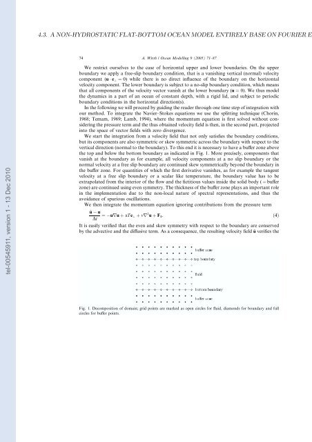
vertical direction (normal to the boundary). To this end it is necessary to have a buffer zone above
the top and below the bottom boundary as indicated in Fig. 1. More precisely, components that
vanish at the boundary as for example, all velocity components at a no slip boundary or the
normal velocity at a free slip boundary are continued skew symmetrically beyond the boundary in
the buffer zone. For quantities of which the first derivative vanishes, as for example the tangent
velocity at a free slip boundary or a scalar like temperature, the boundary value has to be
extrapolated from the interior of the flow and the fictitious values inside the solid body ( ¼ buffer
zone) are continued using even symmetry. The thickness of the buffer zone plays an important role
in the implementation due to the non-local nature of spectral representations, and thus the
avoidance of spurious oscillations.
We then integrate the momentum equation ignoring contributions from the pressure term
~u u
¼ uru þ aT e ? þ mr 2 u þ F 1 : ð4Þ
Dt
It is easily verified that the even and skew symmetry with respect to the boundary are conserved
by the advective and the diffusive term. As a consequence, the resulting velocity field ~u verifies the
Fig. 1. Decomposition of domain; grid points are marked as open circles for fluid, diamonds for boundary and full
circles for buffer points.