Etudes et évaluation de processus océaniques par des hiérarchies ...
Etudes et évaluation de processus océaniques par des hiérarchies ... Etudes et évaluation de processus océaniques par des hiérarchies ...
204 30 CHAPTER 5. DYNAMICS OF THE OCEAN 5.9 Energetics of flow in Geostrophic Equilibrium For the shallow water dynamics the total energy is composed of kinetic and available potential energy (the part of the potential energy which is available in the layered model by reducing the surface anomaly η, if η = 0 everywhere the available potential energy vanishes): E total = E kin + E pot = ρ ∫ H(u 2 + v 2 )dxdy + gρ ∫ η 2 dxdy (5.49) 2 A 2 A = g2 ρ H 2f ∫A ( (∂ 2 x η) 2 + (∂ y η) 2) dxdy + gρ ∫ η 2 dxdy (5.50) 2 A tel-00545911, version 1 - 13 Dec 2010 where we used (eqs. 5.44 and 5.45). If the surface perturbation has the simple form η = η 0 sin(x/L) then the energy is given by: E total = E kin + E pot = gη2 0 4 ∫ A ( Hg f 2 L 2 + 1 ) dxdy (5.51) Were the first term is the kinetic and the second term the available potential energy. We see that in a geostrophic flow the kinetic energy is larger than the available potential energy when the structure is smaller than the Rossby radius R = √ gH/f 2 . So for large geostrophic structures most of the energy is in the potential part and for small structures in the kinetic part. The Rossby radius is of the order of a few thousands of kilometers for the shallow water dynamics of the ocean (the barotropic Rossby radius) but only several tenths of kilometers when the reduced gravity dynamics of the layer above the thermocline are considered (the baroclinic Rossby radius). 5.10 Linear Potential Vorticity and the Rossby Adjustment Problem If we take ∂ x (eq. (5.42)) - ∂ y (eq. (5.41)) we see that: ∂ t ζ + f(∂ x u + ∂ y v) = 0. (5.52) relating vorticity ζ = ∂ x v − ∂ y u to divergence ∂ x u + ∂ y v. Using eq. (5.43) we get: ( ζ ∂ t f − η ) = 0. (5.53) H One usually calls Q lin sw = ζ H − fη H 2 the linear shallow water potential vorticity. The above equations show, that at every location linear shallow water potential vorticity (PV) is conserved, when the dynamics is governed by the linearised shallow water equations. The Rossby adjustment problem considers the adjustment of an initially step-like perturbation (see fig. 5.10), and we would like to know the final, geostrophically balanced state of this perturbation. To this end we use the conservation of potential vorticity and we further require the final state to be in geostrophic equilibrium. The initial potential vorticity is given by sgn(x)(fη 0 )/H 2 the PV of the adjusted state is the same, we thus have, g/(Hf)∂ xx η a − fη a /H 2 = sgn(x)(fη 0 )/H 2 , (5.54) R 2 ∂ xx η a − η a = η 0 sgn(x), (5.55)
205 5.10. LINEAR POTENTIAL VORTICITY AND THE ROSSBY ADJUSTMENT PROBLEM31 ✻ η Z ✲ X Figure 5.5: Initial condition tel-00545911, version 1 - 13 Dec 2010 which has the solution: η a = sgn(x)η 0 (exp(−|x|/R) − 1) (5.56) with R = √ gH/f 2 is called the Rossby radius of deformation. It is the distance, a gravity wave travels in the time f −1 . η ✻ Z Figure 5.6: Adjusted state We have calculated the final geostrophically adjusted state from an initial perturbation using geostrophy and conservation of linear PV, but we have not shown how this adjustment happens. For this a numerical integration of the linear shallow water equations are necessary, eqs. (5.41) – (5.43). Exercise 25: calculate the final velocity field (u,v). Exercise 26: what happens when rotation vanishes? Exercise 27: in section 5.2 we saw that if rotation is vanishing, an initial perturbation of the free surface moves away in both directions leaving an unperturbed free surface and a zero velocity behind. Does this contradict the conservation of linear potential vorticity? Exercise 28: calculate the loss of available potential energy and compare it to the gain in kinetic energy during the adjustment process. Exercise 29: calculate the (barotropic) Rossby radius of deformation (H = 5km), calculate the reduced gravity (baroclinic) Rossby radius of deformation (H = .5km, g ′ = 3. · 10 −2 m/s −2 ) ✲ X
- Page 159 and 160: 4.8. ESTIMATION OF FRICTION LAWS AN
- Page 161 and 162: 4.8. ESTIMATION OF FRICTION LAWS AN
- Page 163 and 164: 4.8. ESTIMATION OF FRICTION LAWS AN
- Page 165 and 166: 4.8. ESTIMATION OF FRICTION LAWS AN
- Page 167 and 168: 4.9. ON THE NUMERICAL RESOLUTION OF
- Page 169 and 170: 4.9. ON THE NUMERICAL RESOLUTION OF
- Page 171 and 172: 4.9. ON THE NUMERICAL RESOLUTION OF
- Page 173 and 174: 4.9. ON THE NUMERICAL RESOLUTION OF
- Page 175 and 176: 4.9. ON THE NUMERICAL RESOLUTION OF
- Page 177 and 178: 4.9. ON THE NUMERICAL RESOLUTION OF
- Page 179 and 180: Quatrième partie tel-00545911, ver
- Page 181 and 182: 175 tel-00545911, version 1 - 13 De
- Page 183 and 184: 177 Contents 1 Preface 5 tel-005459
- Page 185 and 186: 179 Chapter 1 Preface tel-00545911,
- Page 187 and 188: 181 Chapter 2 Observing the Ocean t
- Page 189 and 190: 183 Chapter 3 Physical properties o
- Page 191 and 192: 185 3.3. θ-S DIAGRAMS 11 3.3 θ-S
- Page 193 and 194: 187 3.6. HEAT CAPACITY 13 tel-00545
- Page 195 and 196: 189 3.7. CONSERVATIVE PROPERTIES 15
- Page 197 and 198: 191 Chapter 4 Surface fluxes, the f
- Page 199 and 200: 193 4.2. FRESH WATER FLUX 19 water.
- Page 201 and 202: 195 Chapter 5 Dynamics of the Ocean
- Page 203 and 204: 197 5.2. THE LINEARIZED ONE DIMENSI
- Page 205 and 206: 199 5.4. TWO DIMENSIONAL STATIONARY
- Page 207 and 208: 201 5.6. THE CORIOLIS FORCE 27 Whic
- Page 209: 203 5.8. GEOSTROPHIC EQUILIBRIUM 29
- Page 213 and 214: 207 5.13. A FEW WORDS ABOUT WAVES 3
- Page 215 and 216: 209 Chapter 6 Gyre Circulation tel-
- Page 217 and 218: 211 6.1. SVERDRUP DYNAMICS IN THE S
- Page 219 and 220: 213 6.2. THE EKMAN LAYER 39 In the
- Page 221 and 222: 215 6.3. SVERDRUP DYNAMICS IN THE S
- Page 223 and 224: 217 Chapter 7 Multi-Layer Ocean dyn
- Page 225 and 226: 219 7.3. GEOSTROPHY IN A MULTI-LAYE
- Page 227 and 228: 221 7.5. EDDIES, BAROCLINIC INSTABI
- Page 229 and 230: 223 Chapter 8 Equatorial Dynamics t
- Page 231 and 232: 225 Chapter 9 Abyssal and Overturni
- Page 233 and 234: 227 9.2. MULTIPLE EQUILIBRIA OF THE
- Page 235 and 236: 229 9.3. WHAT DRIVES THE THERMOHALI
- Page 237 and 238: 231 Chapter 10 Penetration of Surfa
- Page 239 and 240: 233 10.2. TURBULENT TRANSPORT 59 If
- Page 241 and 242: 235 10.5. ENTRAINMENT 61 instabilit
- Page 243 and 244: 237 Chapter 11 Solution of Exercise
- Page 245 and 246: 239 65 Exercise 32: The moment of i
- Page 247 and 248: 241 INDEX 67 Transport stream-funct
- Page 249 and 250: Annexe A Attestation de reussite au
- Page 251 and 252: Annexe B Rapports du jury et des ra
- Page 253 and 254: tel-00545911, version 1 - 13 Dec 20
- Page 255 and 256: tel-00545911, version 1 - 13 Dec 20
- Page 257 and 258: 251 utilisés avec pertinence. Sur
- Page 259 and 260: 253
205<br />
5.10. LINEAR POTENTIAL VORTICITY AND THE ROSSBY ADJUSTMENT PROBLEM31<br />
✻<br />
η<br />
Z<br />
✲ X<br />
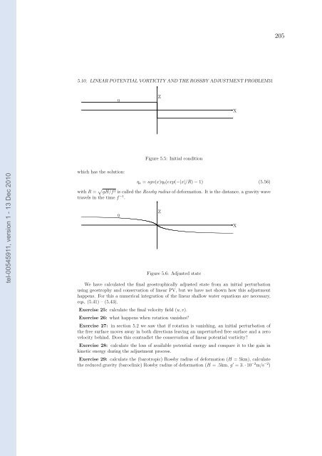
Figure 5.5: Initial condition<br />
tel-00545911, version 1 - 13 Dec 2010<br />
which has the solution:<br />
η a = sgn(x)η 0 (exp(−|x|/R) − 1) (5.56)<br />
with R = √ gH/f 2 is called the Rossby radius of <strong>de</strong>formation. It is the distance, a gravity wave<br />
travels in the time f −1 .<br />
η<br />
✻<br />
Z<br />
Figure 5.6: Adjusted state<br />
We have calculated the final geostrophically adjusted state from an initial perturbation<br />
using geostrophy and conservation of linear PV, but we have not shown how this adjustment<br />
happens. For this a numerical integration of the linear shallow water equations are necessary,<br />
eqs. (5.41) – (5.43).<br />
Exercise 25: calculate the final velocity field (u,v).<br />
Exercise 26: what happens when rotation vanishes?<br />
Exercise 27: in section 5.2 we saw that if rotation is vanishing, an initial perturbation of<br />
the free surface moves away in both directions leaving an unperturbed free surface and a zero<br />
velocity behind. Does this contradict the conservation of linear potential vorticity?<br />
Exercise 28: calculate the loss of available potential energy and com<strong>par</strong>e it to the gain in<br />
kin<strong>et</strong>ic energy during the adjustment process.<br />
Exercise 29: calculate the (barotropic) Rossby radius of <strong>de</strong>formation (H = 5km), calculate<br />
the reduced gravity (baroclinic) Rossby radius of <strong>de</strong>formation (H = .5km, g ′ = 3. · 10 −2 m/s −2 )<br />
✲ X


