Etudes et évaluation de processus océaniques par des hiérarchies ...

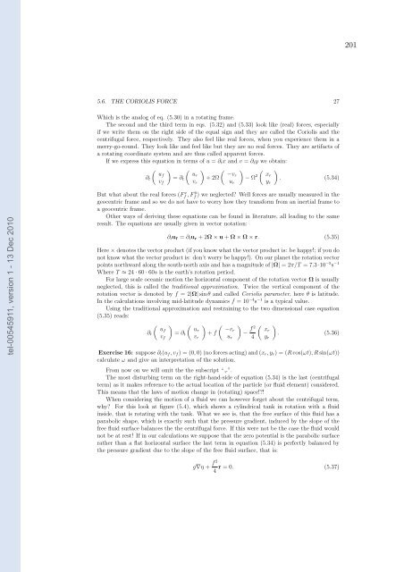
201
5.6. THE CORIOLIS FORCE 27
Which is the analog of eq. (5.30) in a rotating frame.
The second and the third term in eqs. (5.32) and (5.33) look like (real) forces, especially
if we write them on the right side of the equal sign and they are called the Coriolis and the
centrifugal force, respectively. They also feel like real forces, when you experience them in a
merry-go-round. They look like and feel like but they are no real forces. They are artifacts of
a rotating coordinate system and are thus called apparent forces.
If we express this equation in terms of u = ∂ t x and v = ∂ t y we obtain:
∂ t
(
uf
v f
)
= ∂ t
(
ur
v r
)
+ 2Ω
( −vr
u r
)
− Ω 2 (
xr
y r
)
. (5.34)
tel-00545911, version 1 - 13 Dec 2010
But what about the real forces (Ff x,F y f
) we neglected? Well forces are usually measured in the
geocentric frame and so we do not have to worry how they transform from an inertial frame to
a geocentric frame.
Other ways of deriving these equations can be found in literature, all leading to the same
result. The equations are usually given in vector notation:
∂ t u f = ∂ t u r + 2Ω × u + Ω × Ω × r. (5.35)
Here × denotes the vector product (if you know what the vector product is: be happy!; if you do
not know what the vector product is: don’t worry be happy!). On our planet the rotation vector
points northward along the south-north axis and has a magnitude of |Ω| = 2π/T = 7.3·10 −5 s −1
Where T ≈ 24 · 60 · 60s is the earth’s rotation period.
For large scale oceanic motion the horizontal component of the rotation vector Ω is usually
neglected, this is called the traditional approximation. Twice the vertical component of the
rotation vector is denoted by f = 2|Ω| sin θ and called Coriolis parameter, here θ is latitude.
In the calculations involving mid-latitude dynamics f = 10 −4 s −1 is a typical value.
Using the traditional approximation and restraining to the two dimensional case equation
(5.35) reads:
( ) ( ) ( ) ( )
uf ur −vr
∂ t = ∂
v t + f − f2 xr
. (5.36)
f v r u r 4 y r
Exercise 16: suppose ∂ t (u f ,v f ) = (0, 0) (no forces acting) and (x r ,y r ) = (R cos(ωt),Rsin(ωt))
calculate ω and give an interpretation of the solution.
From now on we will omit the the subscript “. r ”.
The most disturbing term on the right-hand-side of equation (5.34) is the last (centrifugal
term) as it makes reference to the actual location of the particle (or fluid element) considered.
This means that the laws of motion change in (rotating) space!?!
When considering the motion of a fluid we can however forget about the centrifugal term,
why? For this look at figure (5.4), which shows a cylindrical tank in rotation with a fluid
inside, that is rotating with the tank. What we see is, that the free surface of this fluid has a
parabolic shape, which is exactly such that the pressure gradient, induced by the slope of the
free fluid surface balances the the centrifugal force. If this were not be the case the fluid would
not be at rest! If in our calculations we suppose that the zero potential is the parabolic surface
rather than a flat horizontal surface the last term in equation (5.34) is perfectly balanced by
the pressure gradient due to the slope of the free fluid surface, that is:
g∇η + f2
r = 0. (5.37)
4