Etudes et évaluation de processus océaniques par des hiérarchies ...

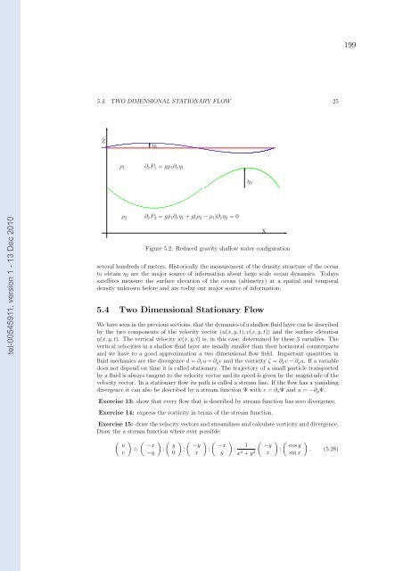
199
5.4. TWO DIMENSIONAL STATIONARY FLOW 25
Z
✻
✻
η 1
η 2
ρ 1
ρ 2
∂ x P 1 = gρ 1 ∂ x η 1
✻
tel-00545911, version 1 - 13 Dec 2010
∂ x P 2 = gρ 1 ∂ x η 1 + g(ρ 2 − ρ 1 )∂ x η 2 = 0
Figure 5.2: Reduced gravity shallow water configuration
several hundreds of meters. Historically the measurement of the density structure of the ocean
to obtain η 2 are the major source of information about large scale ocean dynamics. Todays
satellites measure the surface elevation of the ocean (altimetry) at a spatial and temporal
density unknown before and are today our major source of information.
5.4 Two Dimensional Stationary Flow
We have seen in the previous sections, that the dynamics of a shallow fluid layer can be described
by the two components of the velocity vector (u(x,y,t),v(x,y,t)) and the surface elevation
η(x,y,t). The vertical velocity w(x,y,t) is, in this case, determined by these 3 variables. The
vertical velocities in a shallow fluid layer are usually smaller than their horizontal counterparts
and we have to a good approximation a two dimensional flow field. Important quantities in
fluid mechanics are the divergence d = ∂ x u + ∂ y v and the vorticity ζ = ∂ x v − ∂ y u. If a variable
does not depend on time it is called stationary. The trajectory of a small particle transported
by a fluid is always tangent to the velocity vector and its speed is given by the magnitude of the
velocity vector. In a stationary flow its path is called a stream line. If the flow has a vanishing
divergence it can also be described by a stream function Ψ with v = ∂ x Ψ and u = −∂ y Ψ.
X
✲
Exercise 13: show that every flow that is described by stream function has zero divergence.
Exercise 14: express the vorticity in terms of the stream function.
Exercise 15: draw the velocity vectors and streamlines and calculate vorticity and divergence.
Draw the a stream function where ever possible:
( u
v
) ( ) ( ) ( ) ( )
−x y −y −x
= ; ; ; ;
−y 0 x y
(
1 −y
x 2 + y 2 x
) ( ) cos y
; . (5.28)
sin x