Etudes et évaluation de processus océaniques par des hiérarchies ...

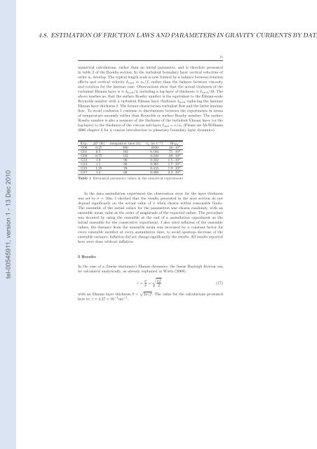
4.8. ESTIMATION OF FRICTION LAWS AND PARAMETERS IN GRAVITY CURRENTS BY DATA
11
numerical calculations, rather than an initial parameter, and is therefore presented
in table 2 of the Results section. In the turbulent boundary layer vertical velocities of
order u ∗ develop. The typical length scale is now formed by a balance between rotation
effects and vertical velocity δ turb ≈ u ∗/f, rather than the balance between viscosity
and rotation for the laminar case. Observations show that the actual thickness of the
turbulent Ekman layer is ≈ δ turb /4, including a log-layer of thickness ≈ δ turb /10. The
above teaches us, that the surface Rossby number is the equivalent to the Ekman-scale
Reynolds number with a turbulent Ekman layer thickness δ turb replacing the laminar
Ekman layer thickness δ. The former characterises turbulent flow and the latter laminar
flow. To avoid confusion I continue to discriminate between the experiments in terms
of temperature anomaly rather than Reynolds or surface Rossby number. The surface
Rossby number is also a measure of the thickness of the turbulent Ekman layer (or the
log-layer) to the thickness of the viscous sub-layer δ sub = ν/u ∗ (Please see McWilliams
2006 chapter 6 for a concise introduction to planetary boundary layer dynamics).
tel-00545911, version 1 - 13 Dec 2010
Exp. ∆T (K) integration time (h) ¯v g (m s −1 ) Re Ek
G00 0.25 360 .0830 .38 · 10 3
G01 0.5 192 0.166 .75 · 10 3
G03 0.75 132 0.249 .88 · 10 3
G12 1.0 96 0.332 1.5 · 10 3
G14 1.1 86 0.365 1.7 · 10 3
G15 1.25 76 0.415 1.9 · 10 3
G17 1.5 66 0.498 2.3 · 10 3
Table 1 Estimated parameter values in the numerical experiments
In the data assimilation experiment the observation error for the layer thickness
was set to σ = 10m. I checked that the results presented in the next section do not
depend significanly on the actual value of σ when chosen within reasonable limits.
The ensemble of the initial values for the parameters was chosen randomly, with an
ensemble mean value at the order of magnitude of the expected values. The procedure
was iterated by using the ensemble at the end of a assimilation experiment as the
initial ensemble for the consecutive experiment. I also tried inflation of the ensemble
values, the distance from the ensemble mean was increased by a constant factor for
every ensemble member at every assimilation time, to avoid spurious decrease of the
ensemble variance. Inflation did not change significantly the results. All results reported
here were done without inflation.
5 Results
In the case of a (linear stationary) Ekman dynamics, the linear Rayleigh friction can
be calculated analytically, as already explained in Wirth (2009):
τ = ν δ = r
νf
2
(17)
with an Ekman layer thickness δ = p 2ν/f. The value for the calculations presented
here is: τ = 2.27 × 10 −4 ms −1 .