

Etudes et évaluation de processus océaniques par des hiérarchies ...
Etudes et évaluation de processus océaniques par des hiérarchies ...
Etudes et évaluation de processus océaniques par des hiérarchies ...

Create successful ePaper yourself
Turn your PDF publications into a flip-book with our unique Google optimized e-Paper software.
134 CHAPITRE 4. ETUDES DE PROCESSUS OCÉANOGRAPHIQUES<br />
554 Ocean Dynamics (2009) 59:551–563<br />
tel-00545911, version 1 - 13 Dec 2010<br />
I used the maximal height H = 200 m for the <strong>de</strong>finition<br />
of the vein Richardson number and a vein Frou<strong>de</strong><br />
number. A vertical Reynolds number is given by Re =<br />
2(Ek Ri tan α) −1 and <strong>de</strong>pends on the Ekman number,<br />
the Richardson number and the slope. This Reynolds<br />
number is the geostrophic velocity multiplied by the<br />
layer thickness and divi<strong>de</strong>d by the vertical viscosity.<br />
The influence of a second scalar, salinity and a nonlinear<br />
equation of state, leading to, e.g. the thermobaric<br />
effect (see Emms 1998), is not consi<strong>de</strong>red here.<br />
2.2 The mathematical mo<strong>de</strong>l<br />
The mathematical mo<strong>de</strong>l for the gravity current dynamics<br />
are the Navier–Stokes equations in a rotating<br />
frame with a buoyant scalar (temperature). I<br />
neglect variations in the stream wise (y) direction of<br />
all the variables but inclu<strong>de</strong> the temperature difference<br />
and all the three components of the velocity<br />
vector, this type of mo<strong>de</strong>l is usually revered to as<br />
2.5 dimensional. This leads to a four-dimensional state<br />
vector <strong>de</strong>pending on two space and the time variable,<br />
(T(x, z, t), u(x, z, t), v(x, z, t), w(x, z, t)).<br />
The domain is a rectangular box that spans 51.2 km<br />
in the x direction and is 492 m <strong>de</strong>ep (z direction). On<br />
the bottom, there is a no-slip and on the top a free-slip<br />
boundary condition. The horizontal boundary conditions<br />
are periodic. The initial condition is a temperature<br />
anomaly which has a <strong>par</strong>abolic shape, which is 200 m<br />
high and 20 km large at the bottom, as <strong>de</strong>scribed in the<br />
previous subsection. The magnitu<strong>de</strong> of the temperature<br />
anomaly is varied in the experiments. The initial velocities<br />
in the gravity current are geostrophically adjusted,<br />
the fluid outsi<strong>de</strong> the gravity current is initially at rest.<br />
The buoyancy force is represented by an acceleration<br />
of strength g ′ cos(α) in the z direction and g ′ sin(α) in<br />
the negative x direction to represent the inclination of<br />
angle α = 1 ◦ . This geom<strong>et</strong>ry represents a rectangular<br />
box that is tilted by an angle of one <strong>de</strong>gree. Such<br />
implementation of a sloping bottom simplifies the numerical<br />
implementation and allows for using powerful<br />
numerical m<strong>et</strong>hods (see next subsection).<br />
2.3 Numerical implementation of mathematical mo<strong>de</strong>l<br />
The numerical mo<strong>de</strong>l used is HAROMOD (Wirth<br />
2005). HAROMOD is a pseudo-spectral co<strong>de</strong>, based on<br />
Fourier series in all the spatial dimensions, that solves<br />
the Navier–Stokes equations subject to the Boussinesq<br />
approximation, a no-slip boundary condition on the<br />
floor and a free-slip boundary condition at the rigid<br />
surface. The time stepping is a third-or<strong>de</strong>r, low-storage,<br />
Runge–Kutta scheme. A major difficulty in the numerical<br />
solution is due to the large anisotropy in the<br />
dynamics and the domain, which is roughly 100 times<br />
larger than <strong>de</strong>ep. There are 896 points in the vertical<br />
direction. For a <strong>de</strong>nsity anomaly larger than 0.75 K,<br />
the horizontal resolution had to be increased from<br />
512 to 2,048 points (see Table 1) to avoid a pile up<br />
of small-scale energy caused by an insufficient viscous<br />
dissipation range, leading to a thermalised dynamics at<br />
small scales as explained by Frisch <strong>et</strong> al. (2008). The<br />
horizontal viscosity is ν h = 5 m 2 s −1 and the horizontal<br />
diffusivity is κ h = 1 m 2 s −1 . The vertical viscosity is<br />
ν v = 10 −3 m 2 s −1 and the vertical diffusivity is κ v =<br />
10 −4 m 2 s −1 . The anisotropy in the turbulent mixing<br />
coefficients reflects the strong anisotropy of the numerical<br />
grid. I checked that the results presented here show<br />
only a slight <strong>de</strong>pen<strong>de</strong>nce on ν h , κ h and κ v by doubling<br />
these constants in a control run. This is no surprise<br />
as the corresponding diffusion and friction times are<br />
larger than the integration time of the experiments.<br />
There is a strong <strong>de</strong>pen<strong>de</strong>nce on ν v , as it d<strong>et</strong>ermines the<br />
thickness of the Ekman layer and the Ekman transport,<br />
which governs the dynamics of the gravity current as<br />
will be shown in Section 3. The vertical extension of<br />
the Ekman layer is a few m<strong>et</strong>res, while the horizontal<br />
extension of the gravity current is up to 50 km. In a<br />
fully turbulent gravity current, the turbulent structures<br />
within the well mixed gravity current will be isotropic<br />
and will therefore measure only a few m<strong>et</strong>res in size.<br />
To simulate a fully turbulent gravity current, 10 5 grid<br />
points would be necessary in the horizontal direction to<br />
obtain an isotropic grid. This is far beyond our actual<br />
computer resources.<br />
2.4 Experiments performed<br />
The <strong>de</strong>nsity anomaly was varied in the experiments.<br />
The integration was stopped when the downslope si<strong>de</strong><br />
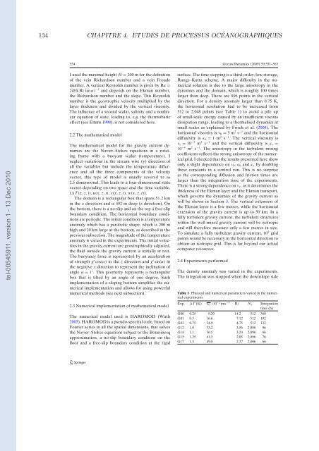
Table 1 Physical and numerical <strong>par</strong>am<strong>et</strong>ers varied in the numerical<br />
experiments<br />
Exp. T (K) v G (10 −2 )ms −1 Ri N x Integration<br />
time (h)<br />
G00 0.25 8.30 14.2 512 360<br />
G01 0.5 16.6 7.12 512 192<br />
G03 0.75 24.9 4.75 512 132<br />
G12 1.0 33.2 3.56 2,096 96<br />
G14 1.1 36.5 3.24 2,096 86<br />
G15 1.25 41.5 2.85 2,096 76<br />
G17 1.5 49.8 2.37 2,096 66


