Etudes et évaluation de processus océaniques par des hiérarchies ...

4.6. ESTIMATION OF FRICTION PARAMETERS AND LAWS IN 1.5D SHALLOW-WATER GRAVI
Ocean Dynamics
tel-00545911, version 1 - 13 Dec 2010
neglect the long-stream variation of the gravity current
and consider only the dynamics of a vertical slice.
Please note that such simplified geometry inhibits largescale
instability and the formation of the large cyclones
and other large-scale features, which is beneficial to our
goal of studying the friction laws due to only small-scale
dynamics.
The gravity current transfers potential energy to
kinetic energy, by sliding down the incline, and looses
energy by friction (dissipation). The down-slope movement
is, thus, “indirectly” determined by friction. This
is exactly what happens to a gravity current in nature,
and it is this dynamic that we like to entangle here.
The difference is, of course, that our gravity current
descends in time and not in space, as in the ocean. This
setup is also used in laboratory experiments and other
numerical simulations (see, e.g. Shapiro and Hill 1997
and Sutherland et al. 2004).
The gravity currents considered here are on an inclined
plane of slope of one degree; the initial profile of
its vertical extension above the inclined ocean floor z =
h(x) = max(H − x 2 /λ, 0) has a parabolic shape with
H = 200 m and λ = 5. · 10 5 m, leading to a gravity
current that is 200 m high and 20 km large. The values
used in the experiment are typical for oceanic gravity
currents (see, e.g. Price and Baringer 1994). If the
gravity current is initially geostrophically adjusted, the
velocity components are given by:
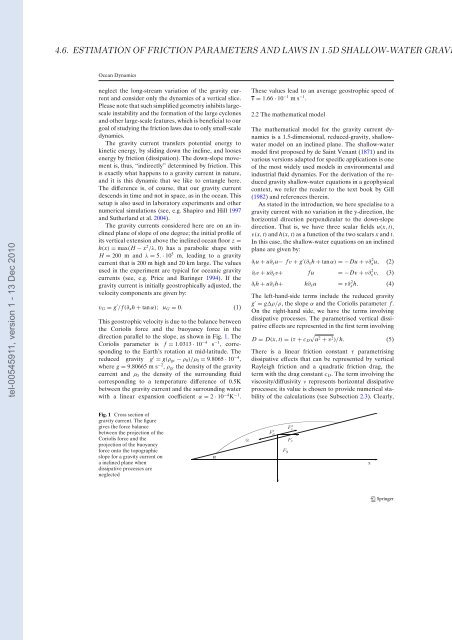
v G = g ′ /f(∂ x h + tan α); u G = 0. (1)
This geostrophic velocity is due to the balance between
the Coriolis force and the buoyancy force in the
direction parallel to the slope, as shown in Fig. 1. The
Coriolis parameter is f = 1.0313 · 10 −4 s −1 , corresponding
to the Earth’s rotation at mid-latitude. The
reduced gravity g ′ = g(ρ gc − ρ 0 )/ρ 0 = 9.8065 · 10 −4 ,
where g = 9.80665 m s −2 , ρ gc the density of the gravity
current and ρ 0 the density of the surrounding fluid
corresponding to a temperature difference of 0.5K
between the gravity current and the surrounding water
with a linear expansion coefficient α = 2 · 10 −4 K −1 .
These values lead to an average geostrophic speed of
v = 1.66 · 10 −1 m s −1 .
2.2 The mathematical model
The mathematical model for the gravity current dynamics
is a 1.5-dimensional, reduced-gravity, shallowwater
model on an inclined plane. The shallow-water
model first proposed by de Saint Venant (1871) and its
various versions adapted for specific applications is one
of the most widely used models in environmental and
industrial fluid dynamics. For the derivation of the reduced
gravity shallow-water equations in a geophysical
context, we refer the reader to the text book by Gill
(1982) and references therein.
As stated in the introduction, we here specialise to a
gravity current with no variation in the y-direction, the
horizontal direction perpendicular to the down-slope
direction. That is, we have three scalar fields u(x, t),
v(x, t) and h(x, t) as a function of the two scalars x and t.
In this case, the shallow-water equations on an inclined
plane are given by:
∂ t u + u∂ x u− fv + g ′ (∂ x h + tan α) = −Du + ν∂x 2 u, (2)
∂ t v + u∂ x v+ f u = −Dv + ν∂x 2 v, (3)
∂ t h + u∂ x h+ h∂ x u = ν∂x 2 h. (4)
The left-hand-side terms include the reduced gravity
g ′ = gρ/ρ, the slope α and the Coriolis parameter f .
On the right-hand side, we have the terms involving
dissipative processes. The parametrised vertical dissipative
effects are represented in the first term involving
D = D(x, t) = (τ + c D
√
u2 + v 2 )/h. (5)
There is a linear friction constant τ parametrising
dissipative effects that can be represented by vertical
Rayleigh friction and a quadratic friction drag, the
term with the drag constant c D . The term involving the
viscosity/diffusivity ν represents horizontal dissipative
processes; its value is chosen to provide numerical stability
of the calculations (see Subsection 2.3). Clearly,
Fig. 1 Cross section of
gravity current. The figure
gives the force balance
between the projection of the
Coriolis force and the
projection of the buoyancy
force onto the topographic
slope for a gravity current on
a inclined plane when
dissipative processes are
neglected
α