Etudes et évaluation de processus océaniques par des hiérarchies ...

112 CHAPITRE 4. ETUDES DE PROCESSUS OCÉANOGRAPHIQUES
APRIL 2008 W I R T H A N D B A R N I E R 811
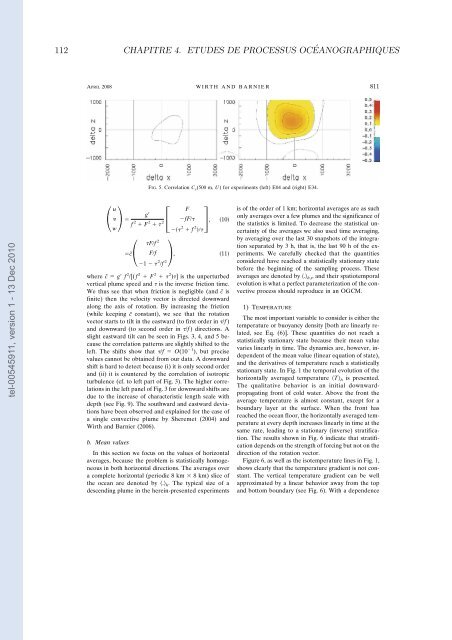
FIG. 5. Correlation C y (500 m, U) for experiments (left) E04 and (right) E34.
tel-00545911, version 1 - 13 Dec 2010
u
w 2
F
g
fF
f 2 F 2
2 f 2
c˜ Ff 2
2 Ff ,
1 2 f
,
10
11
where c˜ g f 2 /[(f 2 F 2 2 )] is the unperturbed
vertical plume speed and is the inverse friction time.
We thus see that when friction is negligible (and c˜ is
finite) then the velocity vector is directed downward
along the axis of rotation. By increasing the friction
(while keeping c˜ constant), we see that the rotation
vector starts to tilt in the eastward (to first order in /f )
and downward (to second order in /f ) directions. A
slight eastward tilt can be seen in Figs. 3, 4, and 5 because
the correlation patterns are slightly shifted to the
left. The shifts show that /f O(10 1 ), but precise
values cannot be obtained from our data. A downward
shift is hard to detect because (i) it is only second order
and (ii) it is countered by the correlation of isotropic
turbulence (cf. to left part of Fig. 3). The higher correlations
in the left panel of Fig. 3 for downward shifts are
due to the increase of characteristic length scale with
depth (see Fig. 9). The southward and eastward deviations
have been observed and explained for the case of
a single convective plume by Sheremet (2004) and
Wirth and Barnier (2006).
b. Mean values
In this section we focus on the values of horizontal
averages, because the problem is statistically homogeneous
in both horizontal directions. The averages over
a complete horizontal (periodic 8 km 8 km) slice of
the ocean are denoted by . h . The typical size of a
descending plume in the herein-presented experiments
is of the order of 1 km; horizontal averages are as such
only averages over a few plumes and the significance of
the statistics is limited. To decrease the statistical uncertainty
of the averages we also used time averaging,
by averaging over the last 30 snapshots of the integration
separated by 3 h, that is, the last 90 h of the experiments.
We carefully checked that the quantities
considered have reached a statistically stationary state
before the beginning of the sampling process. These
averages are denoted by . h,t , and their spatiotemporal
evolution is what a perfect parameterization of the convective
process should reproduce in an OGCM.
1) TEMPERATURE
The most important variable to consider is either the
temperature or buoyancy density [both are linearly related,
see Eq. (6)]. These quantities do not reach a
statistically stationary state because their mean value
varies linearly in time. The dynamics are, however, independent
of the mean value (linear equation of state),
and the derivatives of temperature reach a statistically
stationary state. In Fig. 1 the temporal evolution of the
horizontally averaged temperature T h is presented.
The qualitative behavior is an initial downwardpropagating
front of cold water. Above the front the
average temperature is almost constant, except for a
boundary layer at the surface. When the front has
reached the ocean floor, the horizontally averaged temperature
at every depth increases linearly in time at the
same rate, leading to a stationary (inverse) stratification.
The results shown in Fig. 6 indicate that stratification
depends on the strength of forcing but not on the
direction of the rotation vector.
Figure 6, as well as the isotemperature lines in Fig. 1,
shows clearly that the temperature gradient is not constant.
The vertical temperature gradient can be well
approximated by a linear behavior away from the top
and bottom boundary (see Fig. 6). With a dependence