Etude de la combustion de gaz de synthèse issus d'un processus de ...

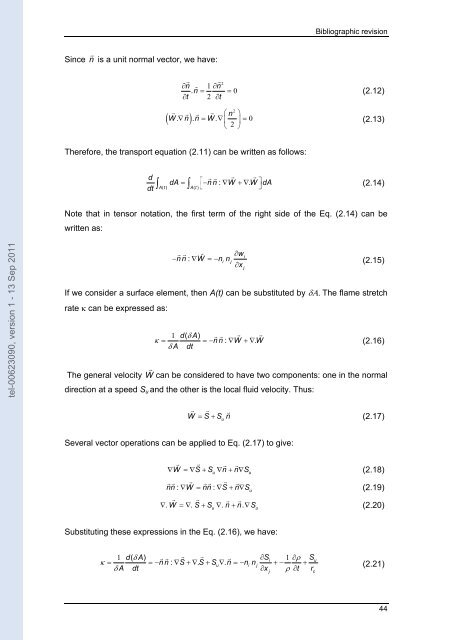
Bibliographic revision
Since n is a unit normal vector, we have:
( )
2
∂n
1 ∂n
. n = = 0
∂t
2 ∂t
∇ = ∇ ⎜ ⎟ = 0
⎝ 2 ⎠
2
n
W. n . n W.
⎛ ⎞
(2.12)
(2.13)
Therefore, the transport equation (2.11) can be written as follows:
d
dt
∫
dA = ⎡−n n : ∇ W +∇.
W ⎤
∫ ⎣
⎦
dA
At ( ) At ( )
(2.14)
Note that in tensor notation, the first term of the right side of the Eq. (2.14) can be
written as:
tel-00623090, version 1 - 13 Sep 2011
−nn:
∇ W = −n n
i
j
∂w
∂x
j
i
(2.15)
If we consider a surface element, then A(t) can be substituted by δΑ. The flame stretch
rate κ can be expressed as:
1 d( δ A)
κ = = −nn: ∇ W +∇.
W
(2.16)
δ A dt
The general velocity W can be considered to have two components: one in the normal
direction at a speed S u and the other is the local fluid velocity. Thus:
W = S + S n
u
(2.17)
Several vector operations can be applied to Eq. (2.17) to give:
∇ W = ∇ S + Su
∇ n+ n∇Su
nn : ∇ W = nn : ∇ S + n∇Su
∇ . W = ∇ . S + S ∇ . n+ n.
∇S
u
u
(2.18)
(2.19)
(2.20)
Substituting these expressions in the Eq. (2.16), we have:
1 d( δA)
∂Si
1 ∂ρ
S
κ = = −nn: ∇ S+∇ . S+ Su∇ . n = − ni nj
+− +
δA dt ∂x ρ ∂t r
j
u
c
(2.21)
44