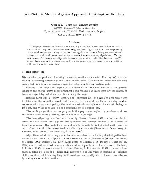
AntNet: A Mobile Agents Approach to Adaptive Routing

AntNet: A Mobile Agents Approach to Adaptive Routing 

Gianni Di Caro and Marco Dorigo 

IRIDIA, Universite Libre de Bruxelles 

50, av. F. Roosevelt, CP 194/6, 1050 - Brussels, Belgium 

Technical Report IRIDIA 97-12 

Abstract 

This paper introduces AntNet, a new routing algorithm for communications networks. 

AntNet is an adaptive, distributed, mobile-agents-based algorithm which was inspired by 

recent work on the ant colony metaphor. We apply AntNet to a datagram network and 

compare it with both static and adaptive state-of-the-art routing algorithms. We ran 

experiments for various paradigmatic temporal and spatial trac distributions. AntNet 

showed both very good performance and robustness under all the experimental conditions 

with respect to its competitors. 

1. Introduction 

We consider the problem of routing in communications networks. Routing refers to the 

activity of building forwarding tables, one for each node in the network, which tell incoming 

data which link to use to continue their travel towards the destination node. 

Routing is an important aspect of communications networks because it can greatly 

inuence the overall network performance: good routing can cause greater throughput or 

lower average delays all other conditions being the same. 

Routing algorithms strongly interact with congestion and admission control algorithms 

to determine the overall network performance. In this work we focus on datagram-like 

networks with irregular topology, the most remarkable example of such networks being the 

Internet, and without congestion or admission control components. 

The routing algorithm that we propose in this paper was inspired by previous works on 

ant colonies and, more generally, by the notion of stigmergy. 

The term stigmergy was rst introduced by Grasse (Grasse, 1959) to describe the indirect 

communication taking place among individuals through modications induced in 

their environment. Real ants have been shown to be able to nd shortest paths using as 

only information the pheromone trail deposited by other ants (Goss, Aron, Deneubourg, & 

Pasteels, 1989; Beckers, Deneubourg, & Goss, 1992). 

Algorithms which take inspiration from ants' behavior in nding shortest paths have 

recently been successfully applied to both combinatorial optimization (Dorigo, Maniezzo, 

& Colorni, 1991; Dorigo, 1992; Dorigo, Maniezzo, & Colorni, 1996; Dorigo & Gambardella, 

1997) and circuit switched communications network problems (Schoonderwoerd, Holland, 

& Bruten, 1997a; Schoonderwoerd, Holland, Bruten, & Rothkrantz, 1997b). In ant colony 

based algorithms, a set of articial ants move on the graph which represents the instance 

of the problem: while moving they build solutions and modify the problem representation 

by adding collected information. 

1

In AntNet, the algorithm we propose in this paper, each articial ant builds a path from 

its source to its destination node. While building the path, it collects explicit information 

about the time length of the path components and implicit information about the load 

status of the network. This information is then back-propagated by another ant moving in 

the opposite direction and is used to modify the routing tables of visited nodes. 

We report on the behavior of AntNet as compared to some eective static and adaptive 

vector-distance and link-state shortest paths routing algorithms (Steenstrup, 1995). 

AntNet shows the best performance and the more stable behavior for all the paradigmatical 

temporal and spatial trac distributions considered. Its best competitor is still another 

new algorithm we introduce. Absolute performance is scored according to a scale dened by 

an ideal algorithm giving an empirical bound. Competitors algorithms performed poorly for 

heavy trac situations and showed more sensitivity tointernal parameters tuning. AntNet, 

on the other hand, has only a small set of tunable parameters and its behavior is very robust 

with respect to their tuning. 

2. Routing Algorithms: an Overview 

The goal of every routing algorithm is to direct trac from sources to destinations maximizing 

network performance while minimizing costs. In this way, the general problem of 

determining an optimal routing algorithm can be stated as a multiobjective optimization 

problem in a non-stationary stochastic environment. Additional constraints are posed by 

the underlying network switching and transmission technology. 

The performance measures that usually are taken into account are throughput and average 

packet delay. The former quantify the quantity of service that the network has been 

able to oer in a certain amount of time, while the latter denes the quality of service 

produced at the same time. 

The precise balance between throughput and average delay will be determined by the 

ow control algorithms operating concurrently with the routing algorithms. Citing (Bertsekas 

& Gallager, 1992) (pag. 367): \the eect of good routing is to increase throughput 

for the same value of average delay per packet under high oered load conditions and to 

decrease average delay per packet under low and moderate oered load conditions". 

Routing algorithms can be at rst broadly classied into centralized or distributed, static 

or adaptive. 

Centralized algorithms can be used only in particular cases. In general, the delays 

necessary to gather information about the network status and to broadcast the routing 

decisions make them unfeasible. 

In static (or oblivious) routers, the path taken by a packet is determined only on the 

basis of its source and destination, without regard to the current network state. This path 

is usually chosen as the shortest one according to some cost criterion, and it can be changed 

to account for faulty links or nodes. 

Adaptive routers are, in principle, more attractive, because they can adapt the routing 

policy to time and spatially varying trac conditions. As a drawback, they can cause oscillations 

in selected paths. This fact can cause circular paths, as well as large uctuations 

in measured performance, especially concerning average delays. In addition, adaptive routing 

can lead more easily to inconsistent situations, associated with node or link failures or 

2

local topological changes. These stability and inconsistency problems are more evident for 

datagram networks than for virtual circuit networks (Bertsekas & Gallager, 1992). In fact, 

in datagram networks every packet selects the path hop by hop. This allows the system to 

react quickly and adapt to changes in routing tables but can also easily lead to an oscillatory 

behavior. Moreover, packets, to choose dierent paths, will likely arrive out-of-order and 

this can be a potential problem that has to be managed in an appropriate way by the underlying 

control protocol. Virtual circuit networks do not exhibit re-ordering problems and 

their (lower) sensitivity to routing tables updates strictly depends on the circuits creation 

rate and holding time. 

Adaptive routers can be broken down in two broad categories: minimal and non-minimal 

(Bolding, Fulgham, & Snyder, 1994). Minimal routers allow packets to choose only minimal 

cost paths, while non-minimal algorithms allow choosing among all the available paths 

following some heuristic strategies. Examples of non-minimal routers are deection routers, 

hierarchical routers, cut-through routers, queuing routers (see for example (Bolding et al., 

1994) and (Bertsekas & Gallager, 1992) for descriptions and references). 

Oblivious and minimal adaptive routing algorithms are the most widely used routing 

paradigms (at least taking in consideration wide-area communication networks). Considering 

dierent perspectives in minimal length paths computation, these algorithms can be 

further classied as optimal routing and shortest path algorithms (Bertsekas & Gallager, 

1992), which are discussed in the following. 

In section 5 we will introduce a novel method, AntNet, that shares the same optimization 

perspective as shortest path algorithms but not their usual implementation paradigms 

(depicted in sect. 2.2). 

2.1 Optimal Routing 

Optimal routing has a network-wide perspective and its objective is to optimize a function 

of all individual link ows (usually this function is a sum of link costs assigned on the basis 

of average packet delays). 

These kind of routing models are called ow models because they try to optimize the total 

mean ow on the network. They can be characterized as multicommodity ow problems, 

where the commodities are the trac ows between the sources and the destinations, the 

cost to be optimized is a function of the ows, subject to the constraints of ow conservation 

at each node and positive owonevery link. It is worth observing that the ow conservation 

constraint can be explicitly stated only if the trac arrival rate is known. 

The routing policy consists of splitting any source-target trac pair at strategic points, 

then shifting trac gradually among alternative routes. This often results in the use of 

multiple paths for a same trac ow between an origin-destination pair. 

Implicit in optimal routing is the assumption that the main statistical characteristics 

of the trac are known and not time-varying. Therefore, optimal routing can be used 

for static and centralized/decentralized routing. It is evident that this kind of solution 

suers all the problems of static routers. In addition, it has an important limitation: the 

optimized cost function hardly can capture all the performance measures we are interested 

in. Therefore, an optimal routing policy will probably determine an unbalanced situation 

among the relative measures of dierent desired performance levels. 

3

2.2 Shortest Path Routing 

Shortest path routing has a source-destination pair perspective. Its objective is to determine 

the shortest path between two nodes, where the link costs are computed following some 

statistical and/or physical description of the link states. Dierently from optimal routing, 

here there is not a global cost function to be optimized, but the route between each node 

pair is considered by itself and no a priori knowledge about the trac process is required 

(of course such knowledge could be fruitfully used). 

If the link cost is static and reects both the transmission capacity of the link and a 

measure of the expected trac load over it, then computed shortest paths will be optimal 

on average for stationary trac situations. Of course, serious loss of eciency could arise 

in case of non-stationary conditions or when it is impossible to make assumptions about 

the trac evolution. 

On the other hand, if costs are assigned in a dynamic way, based on statistical measures 

of the link congestion state, a strong feedback eect is introduced between the routing 

policies and the trac patterns. This can lead to undesirable oscillations, as has been 

theoretically predicted and observed in practice (Bertsekas & Gallager, 1992). 

Considering the dierent content stored in each switch 1 routing table, shortest path 

algorithms can be further subdivided in two classes called distance-vector and link-state 

(Steenstrup, 1995). 

The common behavior of most shortest path algorithms can be depicted as follows. 

1. Each node assigns a cost to each of its outgoing links. This cost can be static or 

dynamic. In the latter case, it is updated in presence of a link failure or on the basis 

of some observed link-trac statistics averaged over a dened time-window. 

2. Periodically and without a required inter-node synchronization, each node sends to all 

of its neighbors a packet of information describing its current estimates about some 

quantities (link costs, distance from all the other nodes, etc.). 

3. Each node upon receiving the information packet updates its local routing table and 

executes some class-specic actions. 

Routing decisions can be made in a deterministic way, choosing the best path indicated 

by the information stored in the routing table, or, adopting a more exible strategy, using 

all the information stored in the table to choose some randomized or alternative path. 

We now describe the features specic of each class; classes dier mainly because of the 

dierent information stored in the routing tables. 

Distance-vector algorithms make use of routing tables consisting of a set of triples of the 

form (Destination, Estimated Distance, Next Hop), dened for all the destinations in 

the network and for all the neighbor nodes of the considered switch. In this case, 

the required topological information is represented by the list of the reachable nodes 

identiers. The average per node memory occupation is of order O(Nn), where N is 

1. The term switch in this context is intended as an alias for network node. It is an appropriate term to 

indicate a virtual device reading the information stored in the local routing table and forwarding the 

packet on the selected outgoing link. 

4

the number of nodes in the network and n is the average connectivity degree (i.e., the 

average number of neighbors nodes considered over all the nodes). 

The algorithm works in an iterative, asynchronous and distributed way. The information 

that every node sends to its neighbors is the list of its last estimates of the 

distances from itself to all the other nodes in the network. After receiving this information 

from a neighbor node j, the receiving node i updates its table of distance 

estimates in the entry corresponding to node j as next hop node. 

Routing decisions at node i are made choosing as next hop node the one satisfying 

the relationship: 

arg minfd ij + D j g 

j 

where d ij is the assigned cost to the link connecting node i with its neighbor j and 

D j is the estimated shortest distance from node j to the destination. 

It can be shown that this process converges in nite time to the shortest paths with 

respect to the used metric if no link cost changes after a given time (Bertsekas & 

Gallager, 1992). 

The above briey described algorithm is known in literature as distributed Bellman- 

Ford (Bellman, 1958; Ford & Fulkerson, 1962; Bertsekas & Gallager, 1992) and it is 

based on the principles of dynamic programming (Bellman, 1957; Bertsekas, 1995). It 

is the prototype and the ancestor of a more wide class of distance-vector algorithms 

(Malkin & Steenstrup, 1995) developed with the aim of reducing the risk of circular 

loops and to accelerate the convergence in case of rapid changes in link costs. 

Link-state algorithms make use of routing tables containing much more information than 

those used in vector-distance algorithms. In fact, at the core of link-state algorithms 

there is a distributed and replicated database. This database is essentially a dynamic 

map of the complete network, describing the details of its components and their 

current interconnections. Using this database as input each node calculates its best 

paths using an appropriate algorithm (usually Dijkstra's (Dijkstra, 1959) algorithm 

is used, but, as described in (Cherkassky, Goldberg, & Radzik, 1994), a wide variety 

of alternative ecient algorithms for shortest paths computations are available). The 

memory space occupation required for each node is in this case of order O(N 2 ). 

In the most common form of link-state algorithm each node acts autonomously, broadcasting 

information about its link costs and states and computing shortest paths from 

itself to all the destinations on the basis of its local link costs estimates and of the 

estimates received from other nodes. Each routing information packet is broadcast to 

all the neighbor nodes that in turn send the packet to their neighbors and so on. A distributed 

ooding (Bertsekas & Gallager, 1992) mechanism supervises this information 

transmission trying to minimize the number of re-transmissions. 

As in the case of vector-distance, the described algorithm is a general template and 

avariety of dierent versions has been implemented to make the algorithm behavior 

more robust and ecient (Moy, 1995). 

5

2.2.1 Links Costs Updates 

We conclude our discussion of shortest paths algorithms stressing the critical role played 

by the choice of an appropriate link costs updating policy in case of non-static costs and 

time-varying trac patterns. 

It is not an easy task to nd the best balance between adaptiveness and stability. Highly 

adaptive metrics can lead to large oscillations with consequent decrease in performance. 

More stable metrics can show a poor responsivity to trac uctuations and congestion 

conditions. Link costs are usually assigned in the following way attempting to reduce 

big variations and taking into account both long-term and short-term statistics of link 

congestion states (Pinelli, 1996): 

1. The rst step is to dene a metric for the links cost evaluation. The cost is updated 

at regular instants t 0 ;t 1 ;t 2 ;:::;t i :::. During every time interval I i =(t i,1 ;t i ] the 

cost is not varied, but \instantaneous" raw cost samples, o t , are calculated (e.g., if the 

metric is a function of the number of bits in the link queue, a new o t is computed at 

every instant t of a packet arrival or departure). Statistics about the values o t ;t2 I i ; 

are recorded and at the end of the time-window I i a mean value of this raw short-term 

cost s ti 

is computed: 

s ti = X t2I i 

o t 

N Ii 

; 

where N Ii is the number of sampled o t values in the time-window I i . 

2. At the same time, all the sampled o t are used to update an exponential mean l t of 

the link cost (long-term cost evaluation) 

lt lt + (o t , l t ) 

3. At the end of each time window the short and the long-term averages are averaged 

and the obtained value is saturated by a linear function with c max and c min as extreme 

values: 

c ti = l ti +s ti 

2 

c ti max( min(ac ti + b; c max );c min ); 

where a and b dene respectively the slope and the oset of the linear saturation 

function. 

4. The obtained cost value c ti is normalized with respect to a maximum admitted variation 

max , and a nal link cost evaluation is obtained. This cost will be held for all 

the duration of the next time interval I i+1 : 

c ti := 

8>< 

>: c t i 

+ sign(c ti , c ti,1 ) max if jc ti , c ti,1 j > max 

c ti 

otherwise: 

Several dierent metrics can be used, we will discuss some of them in section 7. 

6

3. Routing in the Internet 

Several versions of shortest path algorithms have been used during the years for the routing 

management inInternet and in its predecessor, ARPANET. 

The rst routing algorithm on ARPANET, implemented in 1969, was a distributed 

adaptive asynchronous Bellman-Ford algorithm. It used a dynamic link cost metric based 

on measures of trac congestion on the links and in particular of the numberofpackets 

waiting in the link queue. Because this metric led to considerable oscillations, a large 

positive constant was added to stabilize them. Unfortunately, this solution dramatically 

reduced the sensitivity to trac congestion situations. 

These problems led in 1980 to a second version of the routing algorithm in ARPANET, 

known as Shortest Path First (SPF)(McQuillan, Richer, & Rosen, 1980), a link-state routing 

algorithm. A dynamic link cost metric was still used, based on the statistics of the delays 

experienced by data packets. Delays for each single link were computed summing the 

queuing and the transmission and propagation delays. 

This new class of algorithms exhibited more robust behaviors than distance-vector algorithms, 

but in this case too, in case of heavy load conditions, the observed oscillations 

were too large. So, after some revisions concerning the reduction of the allowed variability 

of the links costs (Khanna & Zinky, 1989; Zinky, Vichniac, & Khanna, 1989), the current 

routing algorithm of Internet, Open Shortest Path First (OSPF) (Moy, 1994) is a link-state 

algorithm with a static metric assigned by network administrators. Only temporary or 

permanent topological alterations are ooded in the network. 

This short historical retrospective isintended to highlight the diculties encountered 

in the implementation of adaptive routing algorithms for the Internet. 

The current, essentially static, Internet routing system is not clearly the \best solution", 

it is just the \best compromise" among eciency, stability and robustness that has been 

found so far. Much of the complexity has been moved from the routing system to the 

congestion control system, to avoid high congestion states due to the lack ofamechanism 

for an adaptive ows subdivision among multiple paths. 

But the need for an ecient adaptive routing system is still there, and this need is 

made more evident by forthcoming high-speed networks, which will allow the formulation 

of requests of Quality of Service (QoS) (Crawley, Nair, Rajagopalan, & Sandick, 1996; 

Pinelli, 1996). This means that a user-session can specify the quality of service it needs to 

receive from the network. For example it could specify the maximum and minimum levels 

of throughput, or of end-to-end delay, or the maximum acceptable rate of packets loss, etc. 

In this scenario, it will be of critical importance an ecient adaptive routing policy able to 

support the ow admission control algorithm both in the creation of QoS sessions with very 

strict requirements, and in the global optimization of the network resources usage (Crawley 

et al., 1996). 

It is in this perspective that we developed a robust, adaptive, and distributed routing 

system, AntNet, implemented following alternative schemes with respect to those of classical 

shortest path implementations here briey reported and that showed more than one 

limitation 2 . 

2. Of course, taking in consideration the huge number of interests involved with the Internet (and with 

QoS), a large number of dierent interesting solutions are proposed (see for example the Request For 

7

4. The Communication Network Model 

We focus our experiments on datagram networks with irregular topology and without mechanisms 

for congestion and admission control. This choice has some well-dened motivations. 

First, we want tocheck the behavior of our algorithm and of its competitors in conditions 

which minimize the number of interacting components. In fact, any congestion or admission 

control algorithm has a considerable impact on the network performance and it is dicult 

to evaluate the impact of the control algorithm by itself and of its interactions with the 

routing algorithm. As an example, some authors reported an improvement ranging from 2 

to 30% in various performance measures for real Internet trac (Danzig, Liu, & Yan, 1994), 

changing from the Reno version to the Vegas version of the TCP (Peterson & Davie, 1996) 

(other authors even claimed an improvement ranging from 40 to 70% (Brakmo, O'Malley, 

&Peterson, 1994)). In presence of variations of this entity, it becomes dicult to choose 

the \right" congestion avoidance mechanism and to understand its relationships with the 

underlying routing algorithm. 

Second, wechose to work with datagram networks because using virtual circuits in (highspeed) 

communications networks is tightly bounded to considerations of QoS applications 

(see sec. 3). Therefore, complex admission control algorithms should be introduced. But, 

again, as a rst step we think that it is more reasonable trying to check the validity of 

a routing algorithm reducing the number of components heavily inuencing the network 

behavior. Anyway, our algorithm presents no evident limitations to prevent its use in 

virtual circuit networks. 

In the following, a brief description of the features of the considered network abstraction 

is given. 

The instance of the communication network is mapped on a directed weighted graph 

with N nodes. All the links are viewed as bit pipes characterized by a bandwidth (bits/sec) 

and a transmission delay, and are accessed following a statistical multiplexing scheme. For 

this purpose, every node, of type store-and-forward, (i.e., switch element) holds a buer 

space where the incoming and the outcoming packets are stored. This buer is a shared 

resource among all the queues attached to every incoming and outgoing link of the node. 

All the traveling packets are subdivided in two classes: data and routing packets. All the 

packets in the same class have the same priority, so they are queued and served only on 

the basis of a rst-in-rst-out policy, but routing packets have a greater priority than data 

packets. 

These are fed into the network by applications whose arrival rate is dictated by a selected 

probabilistic model. By application, we mean a process sending data packets from an origin 

node to a destination node. The number of packets to send, their sizes and the intervals 

between them are assigned according to some dened stochastic process. 

A packet reads from the routing table the information about which link to use to follow 

its path toward its target node. When link resources are available, they are reserved and the 

transfer is set up. The time it takes to a packet to move from one node to a neighboring one 

depends on its size and on the link transmission characteristics. If on packet's arrival there 

Comments (RFC) of the Network Working Group at ftp://ds.internic.net), besides those we presented 

in this paper. 

8

is not enough buer space to hold it, the packet is discarded. No arrival acknowledgment 

or error notication packets are generated back to the source. 

After transmission, a stochastic process generates service times for the newly arrived 

packet, that is the delay between its arrival time and the time when it will be ready to be 

put in the buer queue of the selected outgoing link. 

Situations causing a temporary or steady alteration of the network topology or of its 

physical characteristics are not taken into account (link or node failure, adding or deleting 

of network components, etc.). 

We developed a complete network simulator in C++. It is a discrete event simulator 

using as main data structure an event list which holds the next future events. The simulation 

time is a continuous variable and is set by the currently scheduled event. The aim of 

the simulator is to closely mirror the essential features of the concurrent and distributed 

behavior of a generic communication network without sacricing eciency and exibility 

in code development. 

5. AntNet: an Adaptive Agent-based Routing Algorithm 

As shown before, the routing problem is a stochastic distributed multiobjective problem. 

Information propagation delays, and the diculty to completely characterize the network 

dynamics under arbitrary trac patterns, make the general routing problem intrinsically 

distributed. Routing decisions can only be made on the basis of local and approximate 

information about the current and the future network states. 

These features make the problem well suited for a multiagent approach like our AntNet 

system, composed by two sets of homogeneous mobile agents (see (Stone & Veloso, 1996) 

for an agents taxonomy), called in the following forward and backward ants. 

Agents 3 in each set possess the same structure, but they are dierently situated in 

the environment; that is, they can sense dierent inputs and they can produce dierent, 

independent outputs. We can broadly classify them as deliberative agents, because they 

behave reactively retrieving a pre-compiled set of behaviors, and at the same time they 

maintain a complete internal state description. 

The AntNet algorithm can be informally described as follows. 

1. At regular intervals, from every network node s, a mobile agent (that we will call 

forward ant) F s!d , is launched, with a randomly selected destination node d. The 

identier of every visited node k and the time elapsed since its launching time to 

arrive at this k,th node, are pushed onto a memory stack S s!d (k) and inserted in a 

dictionary structure D s!d , carried by the agent. 

2. Each traveling agent selects the next hop node using the information stored in the 

routing table. The route is selected, following a random scheme, proportionally to the 

goodness (probability) of each neighbor node, or, with a tiny probability (exploration 

probability), assigning the same selection probability to each of the neighbor nodes. 

If, in the proportional case, the chosen node has already been visited, a uniformly 

random selection among the neighbors is applied. 

3. In the following, we will use interchangeably the terms Ant and Agent. 

9

3. If a cycle is detected, that is, if an ant is forced to return to an already visited node, 

the cycle's nodes are popped from the ant's stack and all the memory about them is 

destroyed. 

4. When the destination node d is reached, the agent F s!d generates another agent 

(backward ant) B d!s , transferring to it all its memory. 

5. The backward ant takes the same path as that of its corresponding forward ant, but 

in the opposite direction. At each nodek along the path it pops its stack S s!d (k) to 

know the next hop node. 

6. Arriving in a node k coming from a neighbor node f, the backward ant updates the 

following two data structures maintained by every node: 

i) a routing table, organized as in vector-distance algorithms; in the table, a probability 

value P in which expresses the goodness of choosing n as next node when 

the destination node is i, is stored for each pair (i; n) with the constraint 

X 

n2N k 

P in =1;i2 [1;N]; 

N k = fneighbors(k)g; 

ii) a list Trip k ( i ; i2 ) of estimates of arithmetic mean values i and associated 

variances i2 for trip times from node k to all the nodes i in the network (for 

agent-sized packets). This data structure represent a \memory" of the network 

state as seen by nodek. 

These two data structures are updated as follows: 

i) the list Trip k is updated with the values stored in the stack memory S s!d (k); 

all the times elapsed to arrive inevery node k 0 2 S k!d starting from the current 

nodek are used to update the corresponding sample means and variances 

Trip k ( k 0; k 0 2 ); 

ii) the routing table is changed by incrementing the probability P df associated with 

node f when the destination is node d and decrementing the probability P dn 

associated with the other nodes n in the neighborhood for the same destination 

(see g. 1 for an example). 

The update of the routing table happens using the only available feedback signal, that 

is, the trip time experienced by the forward ant. This time gives a clear indication about 

the goodness of the followed route because it is proportional to its length from a physical 

point of view (number of hops, transmission capacity of the used links, processing speed of 

the crossed nodes) and from a trac congestion point of view. This last aspect is extremely 

important: forward ants share the same queues as data packets (backward ants do not, they 

have priority over data to faster propagate the accumulated information), so if they cross a 

congested area, they will be delayed for a long time. This has a double eect: (i) the trip 

time will grow and then back-propagated probability increments will be small and (ii) at 

the same time these increments will be assigned with a bigger delay. In other words, links 

on congested paths will be given only a little, very delayed reward. 

10

Forward Ant (1 4 ) 

1 2 3 

4 

( 1 4) Backward Ant 

Figure 1: Example of the AntNet behavior. The forward ant, F 1!4, moves along the path 1 ! 

2 ! 3 ! 4 and, arrived at node 4, launches the backward ant that will travel in the 

opposite direction. In each nodek; k =2;::: ;4, the backward ant will use the stack 

contents S 1!4(k) to update the values for Trip k ( i ; i 2 ); i =1;:::;(k , 1). At the 

same time the routing table will be updated by incrementing the goodness of the last 

node from where it comes when node 4 is the destination node, that is, incrementing 

P 4j ;j= k +1;j6= 4 and decrementing the values of P for the other neighbors (here not 

shown). The increment will be a function of the trip time experienced by the forward 

ant going from node k to its destination node 4. 

We used the time measure as a reinforcement signal to provide structural and temporal 

credit assignment. The observed times are absolute measures and there is no way we can 

associate with them a precise error measure. We cannot score the trip times according to an 

absolute scale because \optimal" times depend on trac and/or components failure states, 

and they have to be considered from a network wide point of view. 

If the network is in a congested state, all the trip times will score poorly with respect 

to times observed in low load situations, but we should nevertheless be able to understand 

that the network is under congestion and therefore we should give an adequate reward for a 

trip time high from an absolute point of view but signicantly low with respect to the trip 

times observed in the congested situation. We can see that our credit assignment problem 

is the typical one arising in the reinforcement learning eld (Bertsekas & Tsitsiklis, 1996; 

Kaelbling, Littman, & Moore, 1996): we cannot associate the realized performance (trip 

time) with an exact error measure. We can only give \advice" about the goodness of the 

observed trip time on the basis of the estimated mean values for the agent's trip times, 

stored in the list Trip k . 

In light of these considerations, we can detail the procedure followed to update the 

routing tables (we will omit indices when they are not necessary). 

If T is the observed trip time and is its mean value, as stored in the list Trip,we compute 

a raw quantity r 0 measuring the goodness of T , with small values of r 0 corresponding 

to satisfactory trip times, 

r 0 = 

8>< 

>: 

T 

c ; c 1 if T 

c < 1 

1 otherwise: 

r 0 is a dimensionless measure, problem independent, scoring how good is the elapsed trip 

time with respect to what has been on average observed until now. plays the role of a 

11

unit of measure and c is a scale factor (we found that setting c to 2 is a reasonable choice). 

\Out-of-scale" values are saturated to 1. 

A correction strategy is applied to the goodness measure r 0 taking into account how 

reliable is the currently observed trip time with respect to the variance in the so far sampled 

values, that is, considering how stable is the trip time mean value. We say that the 

observations in the mean are stable if = < ; 1 

In this case, a good trip time (i.e., r 0 less than a threshold value t that we set to 0.5) is 

decreased by subtracting a value 

S(;; a)=e ,a 

to the value of r 0 , while a poor trip time is increased adding the same quantity. 

On the other hand, if the mean is not stable, the raw values r 0 cannot be completely 

considered reliable and, in this case, the quantity 

U(;; a 0 )=1, e ,a0 ; 

with a 0 a, is added to a good r 0 value and subtracted from a poor one. In this case, we 

try to avoid following the trac uctuations, with the risk of amplifying them: adding and 

subtracting the value U helps to stabilize them. 

The above correction strategy, for both cases of = values, can be summarized as: 

r 0 r 0 + sign(t , r 0 )sign( , )f(;) ; 

with f being S or U according to the case. The f functions have been chosen as decreasing/increasing 

exponential because both the function and its rst derivative are monotonically 

decreasing/increasing with increasing values of the = ratio. The obtained value of 

r 0 is nally reported on a more compressed scale through a power law, r 0 (r 0 ) h (see below 

for an explanation), and bounded in the interval [0; 1]. 

These transformations from the raw value T to the more rened value r 0 play the role of 

a local estimation of a trac model. More sophisticated and computationally-demanding 

models could be learnt to generate a more eective trac-dependent evaluation measure. 

The situation is similar to that in Actor-Critic systems (Barto, Sutton, & Anderson, 1983): 

araw \reinforcement" signal (the experienced trip time, in our case) is processed by a critic 

module which is learning a model of the underlying process, and then is fed to the learning 

system. 

The obtained value r 0 is used by the current nodek to dene a positive reinforcement, 

r + , for the node f the backward ant comes from, and a negative one, r , , for the other 

neighboring nodes n: 

r + = (1 , r 0 )(1 , P df ) 

r , = , (1 , r 0 )P dn ; n 2N k ;n6= f; 

where P df and P dn are the last probability values assigned to neighbors of node k for 

destination d. In this way, the reinforcements are proportional to the obtained goodness 

measure r 0 and to the previous value of node probabilities. 

12

These probabilities are then increased/decreased by the reinforcement values as follows 

(their sum will still be 1, being r 0 2 [0; 1]): 

P df P df + r + ; P dn P dn + r , : 

It is now clear that the power law rescaling of the r 0 value is equivalent to the denition 

of a learning rate: the scale compression factor and its degree of non linearity determine 

the nal size of the allowed jumps in the probability values. 

The constants (c, a, a 0 , , h, t) used in this section are not problem-dependent and they 

simply dene an appropriate scaling system for the computed values. They have been set 

to the following values: c =2;a=10;a 0 =9;=0:25;h=0:04;t=0:5: 

As a last consideration, notice the critical role played by the stigmergy paradigm for 

agent communication. In fact, each agent is complex enough to solve a single sub-problem 

but the global routing optimization problem cannot be solved eciently by a single agent. 

It is the interaction between the agents that determines the emergence of a global eective 

behavior from the network performance point of view. The key concept in the cooperative 

aspect lies in the way communication among agents happens. The intrinsically distributed 

nature of the problem makes it natural and convenient to use a blackboard type of interagent 

communication, that is, an indirect communication from one agent to all the others 

mediated by the environment. The information locally stored and updated at each network 

node denes the agent input state. Each agent uses it to realize the next node transition 

and, at the same time, it will modify it, modifying in this way the local state of the 

node as seen by future agents. This specic form of indirect communication through the 

environment with no explicit level of agents coordination is called stigmergy (Grasse, 1959; 

Schoonderwoerd et al., 1997a; Stone & Veloso, 1996). We used stigmergy as a way of 

transmitting the information associated with every \experiment" made by each agent (we 

could see our system as a particular instance of an iterated Monte Carlo simulation). 

6. Routing Algorithms Used for Comparison 

To evaluate the performance of AntNet, we selected a set of competitors algorithms from 

the shortest paths class. We wanted to compare our algorithm with the current Internet 

standards and with some improved versions of them closely reecting state-of-the-art for 

routing algorithms. 

The following algorithms have been implemented. 

OSPF: is our implementation of the ocial Internet routing algorithm (Moy, 1994). The 

Internet OSPF has a lot of features for the full network management. Here we are 

only interested in data packet routing in simplied conditions, as described in section 

4. Therefore, the original algorithm is reduced to a simple static shortest path calculation. 

Shortest paths for a sample data packet of size 512 bytes are computed and 

stored in routing tables at the start of the simulation. 

BF: is an implementation of the asynchronous distributed Bellman-Ford algorithm with 

dynamic metrics (Bertsekas & Gallager, 1992). The algorithm has been implemented 

following the guidelines of sections 2.2 and 2.2.1). Vector-distance Bellman-Ford-like 

algorithms are today in use mainly for intradomain routing, because they are used in 

13

the Routing Information Protocol (RIP) (Malkin & Steenstrup, 1995) supplied with 

the BSD version of Unix. 

SPF: is the prototype of link-state algorithms with dynamic metric for link costs evaluations. 

It has been implemented respecting the indications of sections 2.2 and 2.2.1 for 

link-state algorithms. A similar algorithm was implemented in the second version of 

ARPANET (McQuillan et al., 1980) and in its successive revisions (Khanna & Zinky, 

1989). We implemented it with state-of-the-art link costs evaluation and ooding 

algorithms. 

SPF 1F: is the same as SPF but with ooding limited to the rst neighbors. As far as we 

know, this is the rst time that a similar algorithm is presented in literature. It has 

the nice feature that the shortest paths are computed on the basis of locally updated 

information and that the costs of far links are all set to the same value. The algorithm 

makes \myopic" predictions and does not trust delayed information arriving from far 

areas of the network. 

Daemon: is an approximation of an ideal algorithm. It denes an empirical bound on 

the achievable performance. It gives some information about how much improvement 

is still possible. In the absence of any a priori assumption on trac statistics, the 

empirical bound can be dened by an algorithm possessing a \daemon" able to read 

in every instant the state of all the queues in the network and then calculating instantaneous 

\real" costs for all the links and assigning paths on the basis of a network 

wide shortest paths re-calculation for every packet hop. Links costs used in shortest 

paths calculations are the following: 

C li = d li + S p 

+(1, ) S Q(l i ) 

+ 

b li b li 

S Q(li ) 

b li 

; 8i 2 [1;N] 

where d li is the delay for link l i , b li is its bandwidth, S p is the size (in bits) of the data 

packets doing the hop, S Q(li ) is the size (in bits) of the queue of link l i , S Q(li ) is the 

exponential mean of the size of link's queue and it is a correction to the actual size 

of the link queue on the basis of what observed until that moment. This correction is 

weighted by the value set to 0.4. 

Algorithms BF, SPF and SPF 1F use a dynamic metric for link costs. 

following dierent metrics documented in literature (Pinelli, 1996). 

We tried the 

1. The links costs are all set to 1. This is in reality a static metric counting only the 

number of hops (for this and the next metrics, a value of innity is assigned to the 

cost in case of link failure). 

2. The link cost is measured by the link queue occupation during the last time-window. 

More precisely, by the fraction of time of non-empty queue with respect to the emptyqueue 

period. 

3. The link cost is set to the sum of the mean delay of a packet in the link queue plus 

the transmission delay, where the average is done over the last time-window. We call 

this metric DEL. 

14

4. The mean of the transmission time over the link, Tl , and the mean delay in the link's 

queue, D q(l) , are computed over the last time-window. They are used to compute the 

T 

link cost in the following way (Khanna & Zinky, 1989): 1 , 

l 

.We call this metric 

D q(l) 

HND (hop normalized delay). 

5. The link cost is a weighted combination of a pair of the above metrics. We experimentally 

observed that the best combination was given by aweighted average of the 

DEL metric with the HND metric. 

7. Experimental Settings 

The functioning of a communication network is governed by many components which may 

interact in nonlinear and unpredictable ways. Therefore, the choice of a meaningful testbed 

to compare competing algorithms is no easy task. 

A limited set of classes of tunable components are dened and for each of them our 

choices are explained: 

Topology and physical properties of the net. Topology can be dened on the basis 

of a real net instance or it can dened by hand, to better analyze the inuence of 

important topological features (like diameter, connectivity degree, etc.). 

Switches are mainly characterized by their buering and processing capacity, whereas 

links by propagation delay, bandwidth and streams multiplexing scheme. For both, 

fault probability distributions should be dened. 

In our experiments, we used a real net instance, NSFNET, the USA backbone. It is 

composed of 14 nodes and 21 bidirectional links. The topology and the propagation 

delays are shown in g. 2. The bandwidth is 1.5 Mbit/s for every link, the assigned 

link or node fault probability isnull, local buers have innite capacity and links are 

accessed through statistical multiplexing. 

Trac patterns. Trac is dened in terms of open sessions between a pair of active 

applications situated on dierent nodes. Trac patterns can show ahuge variety of 

forms, depending on the characteristics of each session and on their distribution from 

a geographical and from a temporal point of view. 

Each single session is characterized by the number of transmitted packets, and by their 

size and inter-arrival time distributions. More generally, priority, costs and requested 

quality of service should be used to completely characterize a session. 

An application can be characterized by the number of open sessions and by their 

inter-arrival distribution. Applications time arrivals will follow some dened statistics. 

Their geographical distribution over the net is controlled by the probability assigned 

to each node to be selected as an application start or end-point. 

In our experimental settings, we considered only one-session applications, so in the 

following we will use the terms session and application interchangeably. Two models, 

static and dynamic, of temporal trac patterns have been used, modeling respectively 

the case of Constant Bit Rate (CBR) and of Variable Bit Rate (VBR) (Pinelli, 1996). 

15

2 

20 

16 

8 

8 

5 

5 

9 

7 

14 

9 

1 

9 

3 

7 

5 

7 

6 

7 

7 

7 

10 

13 

4 

13 

7 

11 

14 

8 

4 

15 9 

11 

12 

Figure 2: 

NSFNET. Numbers within circles are node identiers, while numbers on links are propagation 

delays in msec. Each edge in the graph represents a pair of directed links. 

In the static model all the sessions start at the beginning of the simulation 

and they last until the end. In this way, we simulate a stationary situation. 

The packet inter-arrival time is a constant value of 150 ms and the packet size 

distribution is a negative exponential with mean 512 bytes. This means a ow 

of 27.3 Kbit/s for each session. 

In the dynamic model, sessions are activated following a negative exponential 

distribution for the inter-arrival times. The mean value of the distribution is 

xed to 15 sec. The total numberofpackets per session, their sizes and their 

inter-arrival times, are negative exponentially distributed, with respectively mean 

values of 50, 512 bytes and 10 sec. In this case, sessions are \bursty" sessions: 

they generate all the packets in a very short time (500 sec on average) after 

their set up, and, after their termination, a long time interval (15 seconds on 

average) elapses before the creation of a new session. Hence, data ows are 

highly irregular both from a temporal and a spatial point of view. 

The geographical distribution of the trac patterns has been modeled considering 

four signicant situations. 

Uniform-deterministic distribution (UD): there are n 1 open sessions between 

any pair of nodes. 

Uniform-random distribution (UR): there are n N 2 open sessions. Start and 

end-points are selected uniformly randomly (i.e., all the nodes have the same 

probability to be selected). 

16

Uniform-deterministic-hot-spots distribution (UDHS): two dierent types of load 

are concurrently present. One is the same as in the UD case, the other is represented 

by a set H of end-points nodes, jHj

\extreme" cases are considered. In fact, for very low, uniform and almost stationary trac 

loads, the six presented algorithms behave almost in the same way and their performance 

is near to optimal. Increasing trac load and/or considering strongly asymmetric spatial 

distributions, it is possible to appreciate dierent behaviors in algorithms performance. We 

report results for some meaningful cases, which well represent algorithm behavior under 

heavy trac conditions. The time length of the simulation has been set to 120 seconds. 

We observed that after this time interval the behavior of the algorithm is already well characterized. 

A 100 seconds of \learning" time has been assigned to the algorithms to learn 

routing tables over the network in absence of trac. 

Reported values are averaged over 10 trials and a bootstrap (Efron & Tibshirani, 1993) 

procedure has been applied to get a better estimate of the variance. In fact, we have to 

take in consideration that large uctuations can appear among trials because similar trac 

situations (in terms of dened trac parameters and distributions) can led to very dierent 

congestion states leading to signicant oscillations in performance. 

In tables 1-8, observed mean values (and their associated standard deviations, in brackets) 

for throughput and mean packet delays are reported. The content of tables 1-4 is 

relative to the case of VBR temporal distribution considered together with the four spatial 

distribution cases, that is, uniform-deterministic, uniform-random, uniform-deterministichot-spots 

and uniform-random-hot-spots. Tables 5-8 follow the same scheme but are relative 

to the CBR case for temporal trac distribution. Experimental conditions are explained 

with detail in tables captions with the following conventions: N UD =number of active sessions 

between all the node pairs; N UR =number of total randomly selected sessions in the 

network, except for hot-spot sessions; N HSN =number of hot-spot nodes; N HSS =number 

of hot-spot sessions. 

From the values in the tables is evident that BF, the algorithm based on distributed 

Bellman-Ford is \out-of-competition", in fact it scores very poorly with respect to the 

others, in all the above situations. Therefore, in the graphs 3-7 its results are not presented. 

Plots refer to some of the cases considered in tables. For each of the considered situations, 

temporal evolution of the average packet delay isshown for every algorithm. Throughput 

plots are not shown because of space reasons and because throughput performance presents 

much less striking dierences than that for packet delays as it is possible to see from the 

tables. For space reasons, not all the data are reported; we chose the most meaningful ones. 

Results about the network usage metric are not reported in detail since no dierences 

among algorithms were observed for both data and routing packets. For all the \pathological" 

cases considered, the trac caused by the routing packets was always negligible 

with respect to trac generated by data packets which caused almost the saturation of the 

network bandwidth. 

18

distribution. N UD =5. 

AntNet OSPF SPF SPF 1F Daemon BF 

Mean Delay (sec) 0.10 (0.01) 0.78 (0.10) 1.41 (0.12) 0.075 (0.03) 0.036 (0.003) 7.85 (2.5) 

Throughput (10 7 bits/sec) 1.348 (0.005) 1.345 (0.007) 1.330 (0.007) 1.347 (0.004) 1.347 (0.005) 0.590 (0.150) 

Table 2: Results for VBR temporal trac distribution and Uniform-random spatial trac distribution. 

N UR = 840: 


Mean Delay (sec) 0.09 (0.01) 0.17 (0.12) 1.00 (0.52) 0.05 (0.04) 0.033 (0.002) 7.00 (2.51) 


Table 3: Results for VBR temporal trac distribution and Uniform-deterministic-hot-spots spatial 

trac distribution. N UD =5;N HSN = 5 and N HSN =5. 


Mean Delay (sec) 0.86 (0.35) 4.80 (2.50) 2.13 (0.35) 1.05 (0.25) 1.05 (0.07) 4.80 (2.03) 


Table 4: Results for VBR temporal trac distribution and Uniform-random-hot-spots spatial trac 

distribution. N UR = 840;N HSS = 5 and N HSN =5. 


Mean Delay (sec) 0.32 (0.12) 3.01 (1.50) 1.94 (0.54) 0.53 (0.18) 0.11 (0.11) 7.48 (2.22) 


Table 5: Results for CBR temporal trac distribution and Uniform-deterministic spatial trac 

distribution. N UD =5. 


Mean Delay (sec) 0.93 (0.20) 5.85(1.43) 3.58 (0.83) 4.96 (1.25) 0.10 (0.03) 4.27 (1.22) 


Table 6: Results for CBR temporal trac distribution and Uniform-random spatial trac distribution. 

N UR = 840: 


Mean Delay (sec) 0.79 (0.18) 4.63 (1.03) 2.01 (0.50) 2.36 (0.67) 0.06 (0.01) 3.90 (1.05) 


Table 7: Results for CBR temporal trac distribution and Uniform-deterministic-hot-spots spatial 

trac distribution. N UD =5;N HSN = 5 and N HSN =5. 


Mean Delay (sec) 3.37 (0.60) 12.00 (2.25) 9.60 (1.44) 11.48 (1.52) 3.28 (0.54) 4.19 (1.97) 


Table 8: Results for CBR temporal trac distribution and Uniform-random-hot-spots spatial trac 

distribution. N UR = 840;N HSN = 5 and N HSN =5. 


Mean Delay (sec) 3.18 (0.75) 10.30 (1.94) 9.42 (0.85) 9.25 (1.00) 2.83 (0.78) 5.09 (1.28) 


19

8 

4.5 

OSPF - 5.cbr.del 

SPF - 5.cbr.del 

7 

4 

6 

3.5 

3 

Average Packet Delay 

5 

4 

3 


2.5 

2 

1.5 

2 

1 

1 

0.5 

0 

0 20 40 60 80 100 120 

Time (sec) 

0 

0 20 40 60 80 100 120 

Time (sec) 

OSPF 

SPF 

7 

0.15 

SPF_1F - 5.cbr.del 

DAEMON - 5.cbr.del 

6 

0.14 

5 

0.13 


4 

3 


0.12 

0.11 

0.1 

2 

0.09 

1 

0.08 

0 

0 20 40 60 80 100 120 

Time (sec) 

0.07 

0 20 40 60 80 100 120 

Time (sec) 

SPF 1F 

Daemon 

1.4 

AntNet - 5.cbr.del 

1.2 

1 


0.8 

0.6 

0.4 

0.2 

0 

0 20 40 60 80 100 120 

Time (sec) 

AntNet 

Figure 3: 

Average packet delay for CBR temporal trac distribution and Uniform-deterministic 

spatial trac distribution. N UD = 5. Note that the graphs have dierent scales. 

20

6 

2.5 

OSPF - 840.cbr.del 

SPF - 840.cbr.del 

5 

2 

Average Packet Delay (sec) 

4 

3 

2 


1.5 

1 

1 

0.5 

0 

0 20 40 60 80 100 120 

Time (sec) 

0 

0 20 40 60 80 100 120 

Time (sec) 

OSPF 

SPF 

3.5 

0.08 

SPF_1F - 840.cbr.del 

DAEMON - 840.cbr.del 

3 

0.075 

2.5 


2 

1.5 


0.07 

0.065 

0.06 

1 

0.5 

0.055 

0 

0 20 40 60 80 100 120 

Time (sec) 

0.05 

0 10 20 30 40 50 60 70 80 90 

Time (sec) 

SPF 1F 

Daemon 

1.2 

AntNet - 840.cbr.del 

1.1 

1 


0.9 

0.8 

0.7 

0.6 

0.5 

0.4 

0.3 

0.2 

0 20 40 60 80 100 120 

Time (sec) 


Figure 4: Average packet delay for CBR temporal trac distribution and Uniform-random spatial 

trac distribution. N UR = 840. Note that the graphs have dierent scales. 

21

7 

3 

OSPF - 5.5.5.vbr.del 

SPF - 5.5.5.vbr.del 

6 

2.5 

5 

2 


4 

3 


1.5 

1 

2 

1 

0.5 

0 

0 20 40 60 80 100 120 

Time (sec) 

0 

0 20 40 60 80 100 120 

Time (sec) 

OSPF 

SPF 

2.2 

0.3 

SPF_1F - 5.5.5.vbr.del 

DAEMON - 5.5.5.vbr.del 

2 

1.8 

0.25 

1.6 


1.4 

1.2 

1 


0.2 

0.15 

0.8 

0.6 

0.1 

0.4 

0.2 

0 20 40 60 80 100 120 

Time (sec) 

0.05 

0 10 20 30 40 50 60 70 80 90 100 

Time (sec) 

SPF 1F 

Daemon 

1.3 

AntNet - 5.5.5.vbr.del 

1.2 

1.1 

1 


0.9 

0.8 

0.7 

0.6 

0.5 

0.4 

0.3 

0.2 

0 20 40 60 80 100 120 

Time (sec) 


Figure 5: 

Average packet delay for VBR temporal trac distribution and Uniform-deterministichot-spots 

spatial trac distribution. N UD =5;N HSS = 5 and N HSN = 5. Note that the 

graphs have dierent scales. 

22

4 

2.5 

OSPF - 840.5.5.vbr.del 

SPF - 840.5.5.vbr.del 

3.5 

2 

3 


2.5 

2 

1.5 


1.5 

1 

1 

0.5 

0.5 

0 

0 20 40 60 80 100 120 

Time (sec) 

0 

0 20 40 60 80 100 120 

Time (sec) 

OSPF 

SPF 

1.8 

0.25 

SPF_1F - 840.5.5.vbr.del 

DAEMON - 840.5.5.vbr.del 

1.6 

0.2 

1.4 

1.2 

0.15 


1 

0.8 

0.6 


0.1 

0.05 

0.4 

0 

0.2 

0 

0 20 40 60 80 100 120 

Time (sec) 

-0.05 

0 20 40 60 80 100 120 

Time (sec) 

SPF 1F 

Daemon 

1.1 

AntNet - 840.5.5.vbr.del 

1 

0.9 

0.8 


0.7 

0.6 

0.5 

0.4 

0.3 

0.2 

0.1 

0 20 40 60 80 100 120 

Time (sec) 


Figure 6: 

Average packet delay for VBR temporal trac distribution and Uniform-random-hotspots 

spatial trac distribution. N UR = 840;N HSN = 5 and N HSN = 5. Note that the 


23

12 

12 

OSPF - 840.5.5.cbr.del 

SPF - 840.5.5.cbr.del 

10 

10 


8 

6 

4 


8 

6 

4 

2 

2 

0 

0 20 40 60 80 100 120 

Time (sec) 

0 

0 20 40 60 80 100 120 

Time (sec) 

OSPF 

SPF 

12 

4 

SPF_1F - 840.5.5.cbr.del 

DAEMON - 840.5.5.cbr.del 

10 

3.5 


8 

6 

4 


3 

2.5 

2 

2 

1.5 

0 

0 20 40 60 80 100 120 

Time (sec) 

1 

0 20 40 60 80 100 120 

Time (sec) 

SPF 1F 

Daemon 

4 

AntNet - 840.5.5.cbr.del 

3.5 

3 


2.5 

2 

1.5 

1 

0.5 

0 

0 20 40 60 80 100 120 

Time (sec) 


Figure 7: 

Average packet delay for CBR temporal trac distribution and Uniform-random-hotspots 

spatial trac distribution. N UR = 840;N HSS = 5 and N HSN = 5. Note that the 


24

Reported results show clearly that AntNet is the best performing algorithm among the 

considered ones (except for the ideal algorithm Daemon). In some cases its superiority is 

evident, in others it performs like the best ones within statistical uctuations. In the CBR 

case, AntNet shows very low delays compared to the others, while in the VBR case, the other 

new algorithm, SPF 1F, presents comparable or slightly better performance. Of course, 

the Daemon algorithm has always the best performance, as expected, and comparing its 

performance with that of AntNet we can see that in the half of the cases AntNet performance 

is almost the same within statistical uncertainties, conrming in this way the excellent 

behavior of our algorithm in accordance with an absolute scale of values. 

\Classical" algorithms (OSPF, SPF and BF) performed poorly with respect to AntNet 

and SPF 1F (limited to the VBR case) and their behavior showed signicant uctuations, 

both in terms of absolute performance and of stability. AntNet was more stable in performance 

and in behavior, that is, always moving rapidly toward a good stable delay value 

after an initial transitory phase. 

9. Summary and Conclusions 

In this paper, we introduced AntNet, a new algorithm for adaptive routing. It is a mobileagents-based 

distributed algorithm using stigmergy as a primitive form of communication 

among agents. 

Its behavior with respect to throughput, mean packet delay and resources usage, has 

been compared to the behavior of other ve shortest paths routing algorithms. As a testbed 

we considered heavy trac conditions for some representative temporal and spatial trac 

distributions for a real network instance. 

AntNet was always, within the statistical uctuations, among the best performing algorithms, 

being in some cases the best one. Dierently from the other algorithms, AntNet 

showed always a robust behavior, being able to rapidly reach a good stable level in performance. 

Moreover, the proposed algorithm has a negligible impact on network resources 

and a small set of robustly tunable parameters. 

The features of the proposed algorithm make itaninteresting alternative to classical 

shortest path routing algorithms. For a more complete validation of the approach, a more 

comprehensive analysis, taking into account congestion and ow control mechanisms, will 

be necessary. 

Acknowledgements 

This work was supported by a Madame Curie Fellowship awarded to Gianni Di Caro 

(CEC-TMR Contract N. ERBFMBICT 961153). Marco Dorigo is a Research Associate 

with the FNRS. 

References 

Barto, A. G., Sutton, R. S., & Anderson, C. W. (1983). Neuronlike adaptive elements that 

can solve dicult learning control problems. IEEE Transaction on Systems, Man and 

Cybernetics, SMC-13, 834{846. 

25

Beckers, R., Deneubourg, J. L., & Goss, S. (1992). Trails and U-turns in the selection of the 

shortest path by the ant Lasius Niger. Journal of Theoretical Biology, 159, 397{415. 

Bellman, R. (1957). Dynamic programming. Princeton University Press. 

Bellman, R. (1958). On a routing problem. Quarterly of Applied Mathematics, 16 (1), 87{90. 

Bertsekas, D. (1995). Dynamic Programming and Optimal Control. Athena Scientic. 

Bertsekas, D., & Gallager, R. (1992). Data Networks. Prentice-Hall. 

Bertsekas, D., & Tsitsiklis, J. (1996). Neuro-Dynamic Programming. Athena Scientic. 

Bolding, K., Fulgham, M. L., & Snyder, L. (1994). The case for chaotic adaptive routing. 

Tech. rep. CSE-94-02-04, Department of Computer Science, UniversityofWashington, 

Seattle. 

Brakmo, L. S., O'Malley, S.W.,&Peterson, L. L. (1994). TCP Vegas: New techniques for 

congestion detection and avoidance. In Proceedings of ACM SIGCOMM 94. 

Cherkassky, B. V., Goldberg, A. V., & Radzik, T. (1994). Shortest Paths Algorithms: 

Theory and Experimental Evaluation. In Sleator, D. D. (Ed.), Proceedings of the 

5th Annual ACM-SIAM Symposium on Discrete Algorithms (SODA 94), pp. 516{525 

Arlington, VA. ACM Press. 

Crawley, E., Nair, R., Rajagopalan, B., & Sandick, H. (1996). A framework for QoS-based 

routing in the internet. Internet Draft (expired in September, 1997) draft-ietf-qosrframework-00, 

Internet Engineering Task Force (IEFT). 

Danzig, P. B., Liu, Z., & Yan, L. (1994). An Evaluation of TCP Vegas by Live Emulation. 

Tech. rep. UCS-CS-94-588, Computer Science Department, University of Southern 

California, Los Angeles. 

Dijkstra, E. W. (1959). A Note on Two Problems in Connection with Graphs. Numer. 

Math, 1, 269{271. 

Dorigo, M. (1992). Optimization, Learning and Natural Algorithms (in Italian). Ph.D. 

thesis, Politecnico di Milano (IT), Dipartimento di Elettronica ed Informatica. 

Dorigo, M., & Gambardella, L. M. (1997). Ant Colony System: A Cooperative Learning 

Approach to the Traveling Salesman Problem. IEEE Transactions on Evolutionary 

Computation, 1 (1), 53{66. 

Dorigo, M., Maniezzo, V., & Colorni, A. (1991). The Ant System: An Autocatalytic 

Optimizing Process. Tech. rep. 91-016, Politecnico di Milano (IT), Dipartimento di 

Elettronica ed Informatica. 

Dorigo, M., Maniezzo, V., & Colorni, A. (1996). The Ant System: Optimization by a colony 

of cooperating agents. IEEE Transactions on Systems, Man, and Cybernetics{PartB, 

26 (1), 29{41. 

26

Efron, B., & Tibshirani, R. (1993). An Introduction to Bootstrap. Chapman & Hall. 

Ford, L., & Fulkerson, D. (1962). Flows in Networks. Prentice-Hall. 

Goss, S., Aron, S., Deneubourg, J. L., & Pasteels, J. M. (1989). Self-organized shortcuts in 

the Argentine ant. Naturwissenschaften, 76, 579{581. 

Grasse, P. P. (1959). La reconstruction du nid et les coordinations interindividuelles 

chez Bellicositermes Natalensis et Cubitermes sp. La theorie de la stigmergie: essai 

d'interpretation du comportement des termites constructeurs. Insectes Sociaux, 6, 

41{81. 

Kaelbling, L. P., Littman, M. L., & Moore, A. W. (1996). Reinforcement Learning: A 

Survey. Journal of Articial Intelligence Research, 4, 237{285. 

Khanna, A., & Zinky, J. (1989). The Revised ARPANET Routing Metric. SIGCOMM 89, 

19 (4), 45{56. 

Malkin, G. S., & Steenstrup, M. E. (1995). Distance-Vector Routing. In Steenstrup, M. E. 

(Ed.), Routing in Communications Networks, chap. 3, pp. 83{98. Prentice-Hall. 

McQuillan, J. M., Richer, I., & Rosen, E. C. (1980). The New Routing Algorithm for the 

ARPANET. IEEE Transactions on Communications, 28, 711{719. 

Moy, J. (1994). OSPF Version 2. Request For Comments (RFC) 1583, Network Working 

Group. 

Moy, J. (1995). Link-State Routing. In Steenstrup, M. E. (Ed.), Routing in Communications 

Networks, chap. 5, pp. 135|157. Prentice-Hall. 

Peterson, L. L., & Davie, B. (1996). Computer Networks: A System Approach. Morgan 

Kaufmann. 

Pinelli, D. (1996). Evaluation of dynamic metrics for IP routing supporting integrated 

services (in Italian). Master's thesis, CEFRIEL, Milano (IT). 

Schoonderwoerd, R., Holland, O., & Bruten, J. (1997a). Ant-like agents for load balancing 

in telecommunications networks. In Proceedings of the First International Conference 

on Autonomous Agents,, pp. 209{216 Marina del Rey, CA. ACM Press. 

Schoonderwoerd, R., Holland, O., Bruten, J., & Rothkrantz, L. (1997b). Load Balancing 

in Telecommunications Networks. Adaptive Behavior, 5 (2). 

Steenstrup, M. E. (Ed.). (1995). Routing in Communications Networks. Prentice-Hall. 

Stone, P., & Veloso, M. (1996). Multiagent systems: a survey from a Machine Learning 

persective. Submitted. 

Zinky, J., Vichniac, G., & Khanna, A. (1989). Performance of the Revised Routing Metric 

in the ARPANET and MILNET. In MILCOM 89. 

27

AntNet: A Mobile Agents Approach to Adaptive Routing

Create successful ePaper yourself

Delete template?

Save as template?