nesting problems: exact and heuristic algorithms - Roderic

DEPARTAMENTO DE ESTADÍSTICA E INVESTIGACIÓN OPERATIVA
PHD THESIS:
NESTING PROBLEMS: EXACT AND HEURISTIC
ALGORITHMS
A Thesis submitted by Antonio Martínez Sykora for the degree of Doctor of Philosophy in the
University of Valencia
Supervised by:
Ramón Álvarez-Valdés Olaguíbel
José Manuel Tamarit Goerlich

To the women of my life: Natalia and Olaya...
3

ACKNOWLEDGEMENTS
This thesis would not have been possible without the generous support of Ramón Álvarez-Valdés Olaguíbel
and Jose Manuel Tamarit Goerlich who strongly supported me.
Special appreciation to professor Enrique Benavent, who spent a lot of time to introduce me into the
Operational Research world.
I want to thank all the examiners, Enriqueta Vercher, José Fernando Oliveira, Maria Antonia Carravilla,
Fran Parreño, Rubén Ruiz and Enrique Benavent for the great effort of reading the thesis carefully and their
for all the observations and corrections.
Many thanks to professors José Fernando Oliveira, Maria Antónia Carravilla and António Miguel Gomes
for supervising me in my research internship in Porto.
Special thanks to Julia Bennell, who spent a lot of her valuable time supervising me in my research
internship in Southampton.
Special thanks to Jonathon Scandrett, who has corrected and improved the English redaction.
I warmly want to thank my family: Juan, Vera, Juanito and Verus.
Finally, very special thanks to Natalia and Olaya for their infinite patience.
5

Contents
1 Introduction to Nesting problems 11
1.1 Introduction . . . . . . . . . . . . . . . . . . . . . . . . . . . . . . . . . . . . . . . . . . . 11
1.2 Types of Nesting Problems . . . . . . . . . . . . . . . . . . . . . . . . . . . . . . . . . . . 12
1.3 Geometry overview . . . . . . . . . . . . . . . . . . . . . . . . . . . . . . . . . . . . . . . 14
1.3.1 Pixel/Raster method . . . . . . . . . . . . . . . . . . . . . . . . . . . . . . . . . . 15
1.3.2 Trigonometry and D functions. . . . . . . . . . . . . . . . . . . . . . . . . . . . . . 17
1.3.3 Non-Fit polygons . . . . . . . . . . . . . . . . . . . . . . . . . . . . . . . . . . . . 19
1.3.4 φ functions . . . . . . . . . . . . . . . . . . . . . . . . . . . . . . . . . . . . . . . 23
1.4 Exact algorithms . . . . . . . . . . . . . . . . . . . . . . . . . . . . . . . . . . . . . . . . 24
1.5 Heuristic algorithms . . . . . . . . . . . . . . . . . . . . . . . . . . . . . . . . . . . . . . . 24
1.6 Instances . . . . . . . . . . . . . . . . . . . . . . . . . . . . . . . . . . . . . . . . . . . . 27
1.6.1 Instances for Nesting Problems . . . . . . . . . . . . . . . . . . . . . . . . . . . . 27
1.6.2 Smaller Nesting instances without rotation . . . . . . . . . . . . . . . . . . . . . . 29
1.6.3 Instances for the two dimensional irregular bin packing problems with guillotine cuts 36
2 Mixed integer formulations for Nesting problems 43
2.1 Formulation GO (Gomes and Oliveira) . . . . . . . . . . . . . . . . . . . . . . . . . . . . . 44
2.2 Formulation HS1 (Horizontal Slices 1) . . . . . . . . . . . . . . . . . . . . . . . . . . . . . 45
2.2.1 Step 1: Complex slices . . . . . . . . . . . . . . . . . . . . . . . . . . . . . . . . . 47
2.2.2 Step 2: Closed slices . . . . . . . . . . . . . . . . . . . . . . . . . . . . . . . . . . 47
2.2.3 Step 3: Horizontal slices . . . . . . . . . . . . . . . . . . . . . . . . . . . . . . . . 49
2.2.4 Non-overlapping constraints . . . . . . . . . . . . . . . . . . . . . . . . . . . . . . 50
2.2.5 Formulation HS1 . . . . . . . . . . . . . . . . . . . . . . . . . . . . . . . . . . . . 50
2.3 Formulation HS2 (Horizontal Slices 2) . . . . . . . . . . . . . . . . . . . . . . . . . . . . . 50
2.3.1 Relative position of pieces . . . . . . . . . . . . . . . . . . . . . . . . . . . . . . . 51
2.3.2 Lifted bound constraints . . . . . . . . . . . . . . . . . . . . . . . . . . . . . . . . 51
2.3.3 Formulation HS2 . . . . . . . . . . . . . . . . . . . . . . . . . . . . . . . . . . . . 53
2.4 Avoiding duplicate solutions . . . . . . . . . . . . . . . . . . . . . . . . . . . . . . . . . . 54
2.5 Computational results . . . . . . . . . . . . . . . . . . . . . . . . . . . . . . . . . . . . . . 54
2.6 Lower bounds . . . . . . . . . . . . . . . . . . . . . . . . . . . . . . . . . . . . . . . . . . 56
3 Branch & Bound algorithms 57
3.1 Branching strategies . . . . . . . . . . . . . . . . . . . . . . . . . . . . . . . . . . . . . . . 58
3.1.1 The Fischetti and Luzzi strategy . . . . . . . . . . . . . . . . . . . . . . . . . . . . 58
3.1.2 Dynamic branching (DB) . . . . . . . . . . . . . . . . . . . . . . . . . . . . . . . . 59
7

3.1.3 Branching on constraints (BC) . . . . . . . . . . . . . . . . . . . . . . . . . . . . . 60
3.1.4 Computational results for the different branching strategies . . . . . . . . . . . . . . 61
3.2 Updating the bounds on the pieces . . . . . . . . . . . . . . . . . . . . . . . . . . . . . . . 66
3.2.1 Method I . . . . . . . . . . . . . . . . . . . . . . . . . . . . . . . . . . . . . . . . 66
3.2.2 Method II . . . . . . . . . . . . . . . . . . . . . . . . . . . . . . . . . . . . . . . . 68
3.3 Finding incompatible variables . . . . . . . . . . . . . . . . . . . . . . . . . . . . . . . . . 68
3.3.1 Incompatibility using the bounds on the pieces . . . . . . . . . . . . . . . . . . . . 69
3.3.2 Incompatibility using the transitivity of the pieces . . . . . . . . . . . . . . . . . . . 69
3.3.3 Computational results of the strategies for updating bounds and finding incompatible
variables . . . . . . . . . . . . . . . . . . . . . . . . . . . . . . . . . . . . . . . . 72
3.4 Results of the complete algorithm . . . . . . . . . . . . . . . . . . . . . . . . . . . . . . . 73
4 Valid Inequalities for the HS2 formulation 77
4.1 X-Y inequalities . . . . . . . . . . . . . . . . . . . . . . . . . . . . . . . . . . . . . . . . . 78
4.1.1 Type I . . . . . . . . . . . . . . . . . . . . . . . . . . . . . . . . . . . . . . . . . . 78
4.1.2 Type II . . . . . . . . . . . . . . . . . . . . . . . . . . . . . . . . . . . . . . . . . 79
4.2 Impenetrability constraints . . . . . . . . . . . . . . . . . . . . . . . . . . . . . . . . . . . 82
4.3 Cliques and Covers . . . . . . . . . . . . . . . . . . . . . . . . . . . . . . . . . . . . . . . 88
4.4 LU-cover inequalities . . . . . . . . . . . . . . . . . . . . . . . . . . . . . . . . . . . . . 97
4.5 Transitivity inequalities . . . . . . . . . . . . . . . . . . . . . . . . . . . . . . . . . . . . . 99
5 Separation algorithms 101
5.1 X-Y inequalities . . . . . . . . . . . . . . . . . . . . . . . . . . . . . . . . . . . . . . . . . 101
5.1.1 Computational results . . . . . . . . . . . . . . . . . . . . . . . . . . . . . . . . . 105
5.2 Impenetrability constraints . . . . . . . . . . . . . . . . . . . . . . . . . . . . . . . . . . . 105
5.2.1 Computational results . . . . . . . . . . . . . . . . . . . . . . . . . . . . . . . . . 106
5.3 Cliques y Covers . . . . . . . . . . . . . . . . . . . . . . . . . . . . . . . . . . . . . . . . 106
5.3.1 Finding all the Cliques . . . . . . . . . . . . . . . . . . . . . . . . . . . . . . . . . 107
5.3.2 SC1 algorithm . . . . . . . . . . . . . . . . . . . . . . . . . . . . . . . . . . . . . 108
5.3.3 SC2 algorithm . . . . . . . . . . . . . . . . . . . . . . . . . . . . . . . . . . . . . 110
5.3.4 Computational results . . . . . . . . . . . . . . . . . . . . . . . . . . . . . . . . . 111
6 Constructive algorithms 113
6.1 Initial models . . . . . . . . . . . . . . . . . . . . . . . . . . . . . . . . . . . . . . . . . . 114
6.2 Studying the initial number of pieces considered (n ini ) . . . . . . . . . . . . . . . . . . . . . 118
6.3 Trunk insertion . . . . . . . . . . . . . . . . . . . . . . . . . . . . . . . . . . . . . . . . . 121
6.4 Alternative objective functions . . . . . . . . . . . . . . . . . . . . . . . . . . . . . . . . . 124
6.5 Conclusions . . . . . . . . . . . . . . . . . . . . . . . . . . . . . . . . . . . . . . . . . . . 127
7 Different approaches to the Local Search 129
7.1 n-insert . . . . . . . . . . . . . . . . . . . . . . . . . . . . . . . . . . . . . . . . . . . . . 129
7.1.1 1-insertion . . . . . . . . . . . . . . . . . . . . . . . . . . . . . . . . . . . . . . . 131
7.1.2 2-insertion . . . . . . . . . . . . . . . . . . . . . . . . . . . . . . . . . . . . . . . 134
7.1.3 3-insertion . . . . . . . . . . . . . . . . . . . . . . . . . . . . . . . . . . . . . . . 135
7.2 Compaction . . . . . . . . . . . . . . . . . . . . . . . . . . . . . . . . . . . . . . . . . . . 136
7.3 1-Compaction . . . . . . . . . . . . . . . . . . . . . . . . . . . . . . . . . . . . . . . . . . 136
8

7.3.1 1-Compaction in one level . . . . . . . . . . . . . . . . . . . . . . . . . . . . . . . 137
7.3.2 1-Compaction into two phases . . . . . . . . . . . . . . . . . . . . . . . . . . . . . 137
7.4 Crossed objectives . . . . . . . . . . . . . . . . . . . . . . . . . . . . . . . . . . . . . . . 138
8 Iterated Greedy Algorithm 143
8.1 Introduction to the Iterated Greedy Algorithm . . . . . . . . . . . . . . . . . . . . . . . . . 143
8.2 Destructive phase . . . . . . . . . . . . . . . . . . . . . . . . . . . . . . . . . . . . . . . . 143
8.3 Constructive phase . . . . . . . . . . . . . . . . . . . . . . . . . . . . . . . . . . . . . . . 144
8.4 Local search procedure . . . . . . . . . . . . . . . . . . . . . . . . . . . . . . . . . . . . . 146
8.4.1 1-insertion modified . . . . . . . . . . . . . . . . . . . . . . . . . . . . . . . . . . 147
8.4.2 2-insertion modified . . . . . . . . . . . . . . . . . . . . . . . . . . . . . . . . . . 148
8.5 IG Algorithm . . . . . . . . . . . . . . . . . . . . . . . . . . . . . . . . . . . . . . . . . . 149
8.6 Computational results . . . . . . . . . . . . . . . . . . . . . . . . . . . . . . . . . . . . . . 150
9 Two dimensional irregular bin packing problems with guillotine cuts 155
9.1 Introduction . . . . . . . . . . . . . . . . . . . . . . . . . . . . . . . . . . . . . . . . . . . 155
9.2 Literature review . . . . . . . . . . . . . . . . . . . . . . . . . . . . . . . . . . . . . . . . 155
9.3 Problem description . . . . . . . . . . . . . . . . . . . . . . . . . . . . . . . . . . . . . . . 157
9.4 Mixed integer formulation for the insertion of one piece . . . . . . . . . . . . . . . . . . . . 158
9.5 Guillotine cut structure . . . . . . . . . . . . . . . . . . . . . . . . . . . . . . . . . . . . . 160
9.6 Rotations and reflections . . . . . . . . . . . . . . . . . . . . . . . . . . . . . . . . . . . . 166
9.7 Constructive algorithm . . . . . . . . . . . . . . . . . . . . . . . . . . . . . . . . . . . . . 167
9.8 Constructive algorithm with two phases . . . . . . . . . . . . . . . . . . . . . . . . . . . . 168
9.9 Embedding an improvement procedure into the constructive algorithm . . . . . . . . . . . . 169
9.10 Computational experiments . . . . . . . . . . . . . . . . . . . . . . . . . . . . . . . . . . . 170
9.11 Conclusions . . . . . . . . . . . . . . . . . . . . . . . . . . . . . . . . . . . . . . . . . . . 176
10 Conclusions and future work 179
9

Chapter 1
Introduction to Nesting problems
1.1 Introduction
Nesting problems are two-dimensional cutting and packing problems involving irregular shapes. This thesis
is focused on real applications on Nesting problems such as the garment industry or the glass cutting. The
aim is to study different mathematical methodologies to obtain good lower bounds by exact procedures and
upper bounds by heuristic algorithms. The core of the thesis is a mathematical model, a Mixed Integer
Programming model, which is adapted in each one of the parts of the thesis.
This study has three main parts: first, an exact algorithm for Nesting problems when rotation for the
pieces is not allowed; second, an Iterated Greedy algorithm to deal with more complex Nesting problems
when pieces can rotate at several angles; third, a constructive algorithm to solve the two-dimensional irregular
bin packing problem with guillotine cuts. This thesis is organized as follows.
The first part is focused on developing exact algorithms. In Chapter 2 we present two Mixed Integer
Programming (MIP) models, based on the Fischetti and Luzzi MIP model [27]. We consider horizontal
lines in order to define the horizontal slices which are used to separate each pair of pieces. The second model,
presented in Section 2.3, uses the structure of the horizontal slices in order to lift the bound constraints.
Section 2.5 shows that if we solve these formulations with CPLEX, we obtain better results than the formulation
proposed by Gomes and Oliveira [32]. The main objective is to design a Branch and Cut algorithm
based on the MIP, but first a Branch and Bound algorithm is developed in Chapter 3. Therefore, we study
different branching strategies and design an algorithm which updates the bounds on the coordinates of the
reference point of the pieces in order to find incompatible variables which are fixed to 0 in the current branch
of the tree. The resulting Branch and Bound produces an important improvement with respect to previous
algorithms and is able to solve to optimality problems with up to 16 pieces in a reasonable time.
In order to develop the Branch and Cut algorithm we have found several classes of valid inequalities.
Chapter 4 presents the different inequalities and in Chapter 5 we propose separation algorithms for some
of these inequalities. However, our computational experience shows that although the number of nodes is
reduced, the computational time increases considerably and the Branch and Cut algorithm becomes slower.
The second part is focused on building an Iterated Greedy algorithm for Nesting problems. In Chapter
6 a constructive algorithm based on the MIP model is proposed. We study different versions depending on
the objective function and the number of pieces which are going to be considered in the initial MIP. A new
11

idea for the insertion is presented, trunk insertion, which allows certain movements of the pieces already
placed. Chapter 7 contains different movements for the local search based on the reinsertion of a given
number of pieces and compaction. In Chapter 8 we present a math-heuristic algorithm, which is an Iterated
Greedy algorithm because we iterate over the constructive algorithm using a destructive algorithm. We have
developed a local search based on the reinsertion of one and two pieces. In the constructive algorithm, for
the reinsertion of the pieces after the destruction of the solution and the local search movements, we use several
parameters that change along the algorithm, depending on the time required to prove optimality in the
corresponding MIP models. That is, somehow we adjust the parameters, depending on the difficulty of the
current MIP model. The computational results show that this algorithm is competitive with other algorithms
and provides the best known results on several known instances.
The third part is included in Chapter 9. We present an efficient constructive algorithm for the two
dimensional irregular bin packing problem with guillotine cuts. This problem arises in the glass cutting
industry. We have used a similar MIP model with a new strategy to ensure a guillotine cut structure. The
results obtained improve on the best known results. Furthermore, the algorithm is competitive with state of
the art procedures for rectangular bin packing problems.
1.2 Types of Nesting Problems
There are several types of Nesting problems depending on the real application the problem comes from. We
define the placement area as a big item and the pieces which have to be arranged into the big item as small
items . There are several different objectives, but the most used one is focused on reducing the total waste
produced.
The most studied problem is the strip packing problem where the width of the strip is fixed and the
objective is based on reducing waste. As all the pieces have to be placed into the strip without overlapping,
minimizing the waste is equivalent to minimizing the total required length. These problems arise in a wide
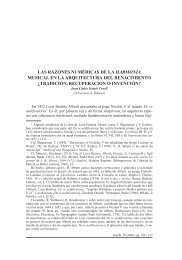
variety of industries like garment manufacturing (see Figure 1.1), sheet-metal cutting, furniture making and
shoe manufacturing.
Figure 1.1: An example from garment manufacturing (taken from Gomes and Oliveira [32])
Two-dimensional Bin Packing Problems consist in placing a set of pieces into a finite number of bins in
12

such a way that the total number of bins is minimized. In some applications, the placement areas into which
the pieces have to be packed or cut can have irregular shapes, as in the case of leather hides for making
shoes. The placement area can have uniform or varying qualities depending on the region, sometimes
including defective parts that cannot be used. In these cases the objective is based on reducing the number
of big items needed to place all the pieces.
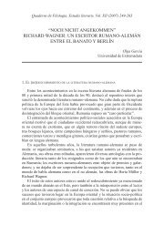
Figure 1.2: An example of a leather cutting instance given by Baldacci et al. [7]
The leather nesting problem (LNP) consists in finding the best layouts for a set of irregular pieces within
large natural leather hides whose contours could be highly irregular and may include holes. According to
the typology presented by Wäscher et al. [70], LNP can be classified as a two-dimensional residual cutting
stock problem (2D-RCSP). Figure 1.2 shows an example of a leather nesting problem.
Heistermann et. al. [33] proposed a greedy algorithm for real instances in the automotive industry. They
consider holes, defects and regions with different levels of quality (quality zones) in the leather hides. Recently,
Alves et. al. [3] have proposed several constructive algorithms, reporting an extensive computational
experiment using two real data sets.
Baldacci et al. [7] use the raster representation to design a heuristic algorithm. They propose an iterative
algorithm based on three different constructive procedures for the Irregular Single Knapsack Problem. They
compare their algorithms on instances defined for two-dimensional strip packing problems, two-dimensional
bin packing problems and real-world leather cutting instances.
Crispin et. al. [21] propose two genetic algorithms using different coding methodologies for shoe manufacturing.
They consider directional constraints for the pieces in given regions of the hides which reduce
the solution space.
There are several publications on the leather nesting problem that do not take quality zones into account.
We can find a heuristic algorithm based on placing the shapes one by one on multiple sheets in Lee et. al
[39], and Yupins and Caijun [72] propose both genetic algorithms and simulated annealing.
Nevertheless, in the literature of Nesting problems the variant with more publications is the two-dimensional
13

strip packing problem where the width of the strip is fixed and minimizing the total required length is the
common objective. This problem is categorized as the two-dimensional, irregular open dimensional problem
in Wäscher et al. [70]. Fowler and Tanimoto [28] demonstrate that this problem is NP-complete and,
as a result, solution methodologies predominantly utilize heuristics. In Sections 1.4 and 1.5 we can find
a literature review on exact methods and heuristic algorithms, respectively. In this thesis we focus on that
problem and both exact and heuristic algorithms are proposed.
One important characteristic of the pieces is their shape. In Nesting problems pieces are irregular and
most frequently polygons. However, there are several publications that consider circular edges. Burke et.
al. [18] propose a generalized bottom-left corner heuristic with hill climbing and tabu search algorithms for
finding a good sequence of the given pieces. Scheithauer et al. [59] use φ-functions to deal with circular
edges. In practice, circular edges of the pieces could be approximated by polygons, so most of the publications
consider the pieces as polygons.
Another feature of the pieces is the allowed angles of rotation: rotation can be free; only specific angles
can be allowed (90 o , 180 o ,...) or rotation is not allowed at all. The angles of rotation can be fixed because
pieces have to respect a given pattern in the stock sheet or due to the structural properties of the material
being cut. In most of the published studies, rotation of the pieces is not allowed or is restricted to several
fixed angles, though there are several studies dealing with free rotation. Xiao Liu and Jia-Wei Ye [41] propose
a constructive heuristic algorithm and Stoyan et al. [63] use φ-functions.
The periodic packing of irregular shapes, also known as regular packing or lattice packing, consists in
packing congruent copies of one shape. Costa et al. [20] propose heuristic algorithms for large-scale periodic
packing. They allow pieces to be rotated freely on the condition that all the pieces must follow the same
orientation (single lattice) or can be rotated 180 o (double lattice). According to the typology by Wäscher
[70], this problem is a two-dimensional irregular IIPP (Identical Item Packing Problem).
Another application of Nesting problems arises in the glass cutting industry. In this case the cutting
process divides the stock sheet (or the given part that is going to be cut) into two different parts. These cuts
are known as guillotine cuts and a direct consequence is that pieces cannot have concavities. Pieces have to
be placed into bins of a fixed width and length, so the objective is to use as few bins as possible to pack all
the pieces.
Finally, we can find several publications on three-dimensional nesting problems. Scheithauer et al. [67]
extend φ-functions to three dimensional objects and Egeblad et al. [26] propose a heuristic algorithm that
can be applied on three-dimensional problems.
1.3 Geometry overview
The main difficulty of solving two-dimensional packing problems appears when we want to ensure that there
is no overlap in the solution or, in the case that there is overlapping, we want to identify the pieces involved.
In this section we review the strategies that can be found in the literature.
First we describe the pixel/raster method, which divides the stock sheet into pixels with each pixel ha-
14

ving a value to indicate if it is used by a piece. This approach has the disadvantage of losing precision when
the problem has irregular pieces. The second method is based on direct trigonometry, using the known D-
functions. The third method uses the Non-Fit Polygons, introduced by Art [5]. The Non-Fit Polygon (NFP)
reduces the problem of identifying whether two polygons overlap to the problem of checking if one point
satisfies any of a subset of linear inequalities. When pieces are allowed to be rotated, the NFPs can be used
only by calculating the NFP of each pair of pieces for each combination of the allowed angles of rotation.
Moreover, when the rotation of pieces is free, the NFP does not work. The Phi-function, introduced by
Stoyan et al. [63], is a generalization of the NFP and gives a measure of the separation between a pair of
pieces. The Phi-function tool is limited by the mathematical complexity needed for it to be defined. However,
it considers the rotation of the pieces. A recent approach is the sentinel method proposed by Macarenhas
and Birgin [47], which also works for a free rotation of the pieces but can be constructed for pieces only
with simple (convex) shapes.
1.3.1 Pixel/Raster method
The idea is to use a matrix where the digits represent a codification of a given area. The stock sheet is
divided into small squares called pixels, obtaining a grid in such a way that the position of each piece in the
strip is given by a set of covered pixels. Each element of the matrix represents a pixel of the strip. Note that
with this representation we lose precision because no pixel is allowed to be covered by two or more different
pieces. Moreover, if we consider a thinner grid then the computational effort would increase considerably.
The codification of the matrix is important, and basically there are three approaches.
Oliveira and Ferreira [50] use a simple codification where each pixel of the matrix takes the value
k = 0, 1, 2, . . . if there are k pieces covering it. Note that if the matrix has a pixel which takes the value 0,
there is no piece covering it. In the case where there is a pixel which takes a value greater than 1, there is
overlapping in the given pixel. In Figure 1.3 we can see the codification of one piece. It is important to
mention that there are pixels which are not completely covered by the piece, but we have to consider that it
is covered in order to ensure that pieces have a non-overlapping configuration, so the corresponding value
in the matrix takes the value 1.
Figure 1.3: Oliveira and Ferreira representation (taken from Bennell and Oliveira [12]).
Segenreich and Braga [60] propose a codification which identifies not only overlapping, but also whether
the pieces are in contact. Their codification uses a 1 for the boundary of the pieces and a 3 for the inner
part. Then, in the pixel-matrix, a pixel with a value greater than 4 indicates that there is overlapping and a
15

pixel with value 2 means that two pieces are in contact but that they do not overlap. If the matrix has all the
elements lower than or equal to 2, then the resulting solution is feasible. In Figure 1.4 we can see two pieces
separately, and then their sum. Note that in the resulting sum we can observe some pixels with a value of
6, meaning that the pieces are in an overlapping position and pixels with the value 4 indicate that, in the
respective pixels, pieces are in a non-feasible position (the boundary of one piece with the inner part of the
other piece).
Figure 1.4: Segenreich and Braga non boolean representation for irregular pieces (taken from Bennell and Oliveira
[12]).
Babu and Babu [6] propose a different idea. Oliveira and Ferreira’s codification, as with Segenreich
and Braga’s, uses 0 for representing the absence of pieces, and a number greater than 0 for the presence of
pieces. Babu and Babu use 0 for representing the inner part of the pieces and a number greater than 0 for
the adjacent pixels. These adjacent pixels are enumerated from right to left in increasing order, starting with
1 at the right of the piece. In Figure 1.5 we can observe how they represent a piece with a hole. The two
central pixels with values 1 and 2 represent the hole in the piece.
Figure 1.5: Babu and Babu representation (taken from Bennell and Oliveira [12]).
The Babu and Babu codification generalizes the shape of the stock sheet. The big item where we have
to arrange the small items can be an irregular polygon and can also have holes which cannot be used by any
piece. One advantage of this codification is that the code of each pixel represents the number of pixels needed
to push the represented piece to the right in order to make the solution possible. In that way, in a given
configuration it is easy to calculate the compaction of the pieces in the bottom-left corner of the strip. The
16

disadvantage of this approach is an increase in the computational effort needed to update the pixel matrix
and its complexity.
1.3.2 Trigonometry and D functions.
This method considers the pieces as polygons. An important advantage when we use polygons for representing
the pieces is the precision that we gain when we deal with irregular pieces. Note that in the pixel/raster
method, precision depends on the accuracy used when defining the grid. However, when we use polygons
we can approximate each piece as much as is necessary.
On the other hand, in the pixel/raster method the amount of required information depends on the area
of the pieces. When the pieces are larger the pixel matrix is more complex and it is harder to update it. If
we use polygons, the amount of required information increases with the number of vertices of the polygons
used for representing the pieces.
The main problem of using polygons appears when we want to guarantee that pieces do not overlap.
The first idea that comes to mind is based on direct trigonometry. There are known tools that allow us to
identify when two segments intersect or if a given point is placed inside a given polygon. These tools are
more complex compared with the pixel/raster method. In fact, the computational time of the pixel/raster
method is quadratic on the size of the pixel matrix, and when we use direct trigonometry the computational
time is exponential on the number of edges of the polygons.
In what follows we are going to present an approach using trigonometry to evaluate whether two polygons
overlap. In Figure 1.6(a) we can observe that if two polygons overlap, then their respective enclosed
rectangles also overlap. Figure 1.6(b) shows that if any two edges intersect, then the rectangles whose diagonal
is one of these edges also overlap.
Figure 1.6: (a) If two polygons overlap, then their respective enclosed rectangles also overlap. (b) If two edges
intersect, then the rectangles whose diagonal is one of the edges also overlap (taken from Bennell and Oliveira [12]).
If the enclosing rectangles of two given polygons do not overlap, then the polygons are not in a overlapping
position. This is much easier to check than checking if two complex polygons overlap. Then, in
order to know whether two pieces overlap or not, the first step is to check if the enclosed rectangles overlap.
Ferreira et. al. [4] study the reduction of checking the feasibility of one given solution by first applying the
17

study of the enclosed rectangles of each pair of pieces, which ranges between 90.7% and 97.6% of the pairs.
Furthermore, if we also analyze the edges, the reduction ranges between 96% and 99.4%. Obviously, the
complexity of the polygons reduces the effectiveness of the study of the enclosing rectangles, but Ferreira et
al. never obtain a reduction percentage lower than 90%.
In order to check if two polygons overlap, Bennell and Oliveira [12] give a set of hierarchical tests.
TEST 1:
Do the bounding boxes of the polygons overlap?
YES
❄
TEST 2:
For each pair of edges from different polygons, do their respective
bounding boxes overlap?
YES
❄
TEST 3:
For each pair of edges from different polygons, does the edge
analysis indicate an intersection?
✲
NO
✲
YES
NO
❄
THE POLYGONS
DO NOT OVER-
LAP
THE POLYGONS
OVERLAP
✻
✛
NO
❄
TEST 4:
For one vertex of each polygon, does that vertex reside inside the
other polygon?
YES
NO
Figures 1.7 (a) and (b) show, respectively, negative answers for Tests 1 and 2. An example of an affirmative
answer is shown in Figures 1.7 (c) and (d), and in Figure 1.7 (e) we can see both possibilities for Test 4.
Figure 1.7: Different cases of the relative position between two pieces (taken from Bennell and Oliveira [12]).
Preparata and Shamos [54] propose a test to identify if a given point is inside a polygon. This test is
useful to solve Test 4. In order to answer Test 3, we can use the known D functions, which are an efficient
18

tool to obtain the relative position between two edges.
D ABP = ((X A − X B )(Y A − Y P ) − (Y A − Y B )(X A − X P )) (1.1)
D functions were introduced by Konopasek [38] and give the relative position between one point, P, with
respect to an oriented edge, AB, see Figure 1.8.
Figure 1.8: Interpretation of the D functions (taken from Bennell and Oliveira [12]).
These functions come from the equation of the distance from a point to a line. The interpretation is the
following one:
• If D A BP > 0, then point P is placed to the left of segment AB.
• If D A BP < 0, then point P is placed to the right of segment AB.
• If D A BP = 0, then point P is placed on the segment AB.
We have to consider the origin of the coordinate axis in the bottom-left corner, i.e. the X axis always
increases to the right and the Y axis increases upward. It is possible to use these functions to study the
relative position between two segments with given orientations. Mahadevan [43] gives a complete study for
differentiating all the cases.
1.3.3 Non-Fit polygons
Nowadays, the Non-Fit polygon (NFP) is the most widely used and effective tool. The idea of the NFP is
the study of the different relative positions between one polygon B, with respect to another polygon A, such
that both polygons are in a touching position without overlapping, i.e. the NFP studies all the positions of
polygon B in which it touches polygon A. This concept was introduced by Art [5].
We denote by P A the reference point of polygon A and P B denotes the reference point of polygon B. Let
us consider that both reference points are in the bottom-left corner of the enclosing rectangle of their respective
polygons. The NFP of pieces A and B, denoted by NFP AB , is the region in which the reference point of
polygon B cannot be placed because it would overlap polygon A. To build it, P A is placed at the origin and
P B slides around polygon A in such a way that there is always a point of polygon B touching the border of
polygon A. The left-hand side of Figure 1.9 shows several positions of polygon B (triangle) moving around
polygon A (square). The right-hand side of the figure shows NFP AB , the forbidden region for placing P B ,
relative to P A , if overlapping is not allowed. Note that NFP BA matches NFP AB with a rotation of 180 o .
Cuninghame-Green [22] proposes an algorithm to obtain the NFPs of convex pieces. In a first step, a
different orientation is assigned to each polygon as is shown in Figure 1.10 (a). Then, fixing the position
of polygon A at the origin in a counterclockwise orientation, all the edges of both polygons are sorted by
19

B
A
(a) Piece B moves around A
(b) NFP AB
Figure 1.9: Building the NFP of pieces A and B
A
B
(a) Orientation of the polygons (b) Different slopes (c) NFP AB
Figure 1.10: Building NFP of convex pieces
non-increasing slope, see Figure 1.10 (b). Finally, all the edges have to be drawn in the corresponding order,
thus obtaining the NFP AB (Figure 1.10 (c)).
When one or both polygons are non-convex, the construction of the NFP is more complex. Figure 1.11,
taken from Bennell and Oliveira [12], shows complicated cases. In Figure 1.11(a), piece B has some feasible
positions within the concavity of A and therefore NFP AB includes a small triangle of feasible placements
for the reference point of B. In Figure 1.11(b), the width of B fits exactly into the concavity of A and its
feasible positions in the concavity produce a segment of feasible positions for the reference point of B in
NFP AB . In Figure 1.11(c), there is exactly one position in which B fits into the concavity of A and then
NFP AB includes a single feasible point for the reference point of B.
B
A
NFP AB
A
B
NFP AB
B
A
NFP AB
(a)
(b)
(c)
Figure 1.11: Special cases of NFP when non-convex pieces are involved (taken from Bennell and Oliveira [12])
20

In this thesis we assume that for each pair of pieces i, j, NFP i j is given by a polygon and, if that is the
case, by a set of points (as in Figure 1.11(c)), a set of segments (as in Figure 1.11(b)) or a set of enclosed
polygons (as in Figure 1.11(a)).
Algorithms to calculate NFPs
Sliding Algorithm
Mahadevan [43] proposes a sliding algorithm in order to obtain the NFP. Let A and B be two pieces and P A
and P B be their respective reference points. In order to obtain NFP AB , we first need an initial position of the
pieces that guarantees the touching position without overlapping. To ensure that, we match the maximum
value of the Y coordinate of B with the minimum value of the Y coordinate of A. The reference point of
B in this position is going to be the first vertex of NFP AB . In the case that there is more than one position
satisfying the previous condition, then the initial vertex will be the point located further to the left in order
to ensure that the initial vertex is a vertex of NFP AB .
Then, in Figure 1.12 we can see that there are three different possibilities for the first movement of B:
• Case (a): The slope of edge (a j , a j+1 ) is lower than the slope of edge (b j , b j+1 ). In that case, b j slides
over the edge (a j , a j+1 ).
• Case (b): The slope of edge (b j , b j+1 ) is lower than the slope of edge (a j , a j+1 ). In that case, a j slides
over the edge (b j , b j+1 ).
• Case (c): Both edges, (a j , a j+1 ) and (b j , b j+1 ), have the same slope. In that case, both glides of cases
(a) and (b) are done.
Figure 1.12: Different cases to begin to slide piece B around piece A (taken from Bennell and Oliveira [12]).
Mahadevan uses the D functions in order to know the inner part of the NFP AB defined by the side of
the segment which is obtained by sliding a complete combination of a vertex-edge of pieces A and B. In the
event that any piece has a concavity, when one vertex slides completely over one edge, the polygons could
be in an overlapping position, see Figure 1.13. In that case, the glide corresponds to the minimum distance
from the starting point to the intersection point of both polygons, which matches with the maximum distance
available for sliding B along the edge such that no overlaps exist with piece A.
The sliding algorithm only works for pairs of polygons that are relatively simple connected polygons.
For example, in Figure 1.11 this algorithm does not find the hole in (a) or the point of (c)).
21

Figure 1.13: Projection of B when it is moved over the edge of A (taken from Bennell and Oliveira [12]).
Whitwell [71] proposes an extension of the sliding algorithm in order to identify the holes. He studies
if there is any edge of any polygon which is not traveled over, i.e. the edge is not used for sliding any
point in the Mahadevan algorithm. If there is any relative position for the non-visited edges such that nonoverlapping
is produced, then there is a hole in the NFP AB . This hole can be obtained in a similar way, using
a glide as above, whose result is the border of the hole. The Whitwell algorithm first applies the Mahadevan
sliding algorithm, but the considered edges are flagged. If there is any non-flagged edge, we can suppose,
without loss of generality, that it belongs to A and each vertex of B is checked to see if it can slide along this
edge without producing an overlap. That can be studied by checking if the two edges whose intersection
defines the given vertex of B are both to the left of the given edge of A. In the case that one or both of them
are placed to the left of the edge of A, then there is no feasible glide between A and B such that the given
vertex of B could touch the given edge of A, see Figure 1.14.
Figure 1.14: (a) b i and b j are both on the right of edge a, (b) b i is on the left and b j is on the right of a, (c) b i an b j
are both on the left of a (taken from Bennell and Oliveira [12]).
Let us suppose that there is one vertex of B such that the two incident edges are both to the right of edge
a, as shown in Figure 1.14 (a). In that case it is necessary to study whether there are some positions in which
to place this vertex over the edge a which produce an overlap of pieces A and B. In order to check this,
Whitwell uses a similar structure to the Mahadevan algorithm. Figure 1.15 shows an example of how the
Whitwell algorithm works in order to find a feasible initial point starting from an overlapping position. Obviously,
when the shapes of the pieces are more complex, having more edges and concavities, this approach
will need more computational effort.
The Minkowski sum
The concept and theory of Minkowski operations comes from the more general field of morphology. The
morphological operation that forms the basis of this technique for finding the NFP is termed dilation. Dilation
grows the image set A through vector addition with set B, and is denoted as A/B. The dilation operator
22

Intersección más próxima
Figure 1.15: The Whitwell method for finding feasible initial points (taken from Bennell and Oliveira [12]).
may also be called the Minkowski sum, defined as follows.
Let A and B be two arbitrary closed sets of vector points in R 2 . S is the resulting sum of adding all the
vector points in A to those in B. Then the Minkowski sum, S , is defined as
S = A ⊕ B = {a + b | a ∈ A, b ∈ B}.
The union of geometric translations of sets can also define the Minkowski sum. If A b denotes set A translated
by vector b, then
⋃
S = A ⊕ B = A b .
Stoyan and Ponomarenko [64] first formalized the relationship between Minkowski sums and NFPs,
providing a rigorous proof in their paper. They termed the NFP as the hodograph. Proof of this relationship
is also discussed in Milenkovic et al. [48] and Bennell [8], who describe it as the Minkowski difference. In
order to use the Minkowski sums and its relationship with the NFP, the realization of the above definition
needs to be formulated into a procedure to obtain the NFP. Ghosh [30] develops a set of Boundary Addition
Theorems for both the convex and non-convex cases that underpin his method of obtaining the Minkowski
sum. That shows that there is sufficient information in the boundary of the polygons to obtain the boundary
of the Minkowski sum. The theorems also support the use of slope diagrams, which form the basis
of his approach, for representing the Minkowski sum. Ghosh [30] provides a detailed explanation of these
theorems and Bennell [8] provides a discussion of the approach with respect to the NFP. In a Bennell et al.
[12] tutorial we can find easy examples of Ghosh’s idea. Recently, Bennell et al. [61] propose an efficient
algorithm to calculate the NFPs using Minkowski sums based on the principles defined by Ghosh.
b∈B
1.3.4 φ functions
The φ function is a topology concept. This tool can be viewed as a generalization of the NFPs, whose
purpose is to represent all the mutual positions of two pieces, which can be polygons or pieces with curved
lines. In Bennell et al. [14] an extensive tutorial on the φ functions and φ objects can be found.
The φ function is a mathematical expression which describes the interaction between two geometrical
objects in such a way that the positions of the objects are the input and a real value is the output. This value
can be viewed as the distance between the objects: if the value is 0, the pieces are touching each other; if
the value is positive, the pieces are separated; and if the value is negative, the pieces overlap.
Stoyan et al.[63] use the φ functions to solve the non-overlapping problem for Nesting problems. They
consider problems with several copies of one and two pieces. In Stoyan et al. [66] this idea is applied to
23

3-dimensional Nesting problems. In this case, they use the φ functions not only to know if a given solution
is feasible, but also to define the mathematical model.
For basic pieces in two dimensions, a φ function class is already defined (see Stoyan et al. [68]). When
dealing with more complex pieces, each piece can be decomposed into convex polygons or basic pieces,
which correspond to a wide set of fixed-orientation bi-dimensional objects, see Stoyan et al. [65]. Scheithauer
et al. [59] study the different combinations of basic pieces with circular segments. Stoyan et al. [67]
and [66] apply this concept to the 3-dimensional case.
There is a close relation between the φ function and the NFP and the Minkowski sum. When the rotation
of both pieces and the position of one of the pieces is fixed, the set of points such that the value of the φ
function is 0 describes the NFP. However, the φ function has more information because it is not necessary
to fix one of the pieces, and also gives an overlapping measure.
1.4 Exact algorithms
Since Nesting problems are harder than rectangular packing problems, which are already NP-hard, we find
mostly heuristic algorithms in the literature. Gomes and Oliveira [32] propose a mixed integer programming
model (MIP model) for pieces with a fixed orientation. They use that model to solve the compaction and
the separation problems embedded into a heuristic algorithm. The compaction problem consists in finding
a better layout from a feasible layout without changing the relative positions between the pieces. The separation
problem tries to transform an unfeasible layout into a feasible solution by minimizing the increase in
the required length. In Gomes and Oliveira [32], the non-overlapping constraints are modeled using binary
variables and big-M constants. In each case the binary variables expressing the relative position of the pieces
are fixed according to certain heuristic rules and the MIP model is transformed into a linear problem.
The only exact algorithm that can be found in the literature is proposed by Fischetti and Luzzi [27]. They
develop a Mixed Integer Programming MIP model and a branching strategy which is used with CPLEX. The
Fischetti and Luzzi MIP non-overlapping constraints use tighter coefficients instead of big-M constants.
The branching strategy is based on separating pieces by blocks, that is, when a block of n pieces is already
separated then the next piece which overlaps with it is separated from the pieces of the block. Their exact
algorithm has been tested on three instances, glass1, glass2 and glass3 with 5, 7 and 9 pieces, respectively.
These instances are broken glass problems, for which the optimal solution has 100% utilization. Fischetti
and Luzzi [27] are able to prove optimality only for instances glass1 and glass2.
1.5 Heuristic algorithms
Bennell and Oliveira [13] in their tutorial in irregular shape packing problems provide an introduction to
heuristic solution methods. There are two ways of dealing with nesting problems: working with partial solutions
and working with complete solutions. The first approach represents the construction of a layout piece
by piece and in some cases can produce reasonable quality solutions at little computational cost. The second
approach works with complete solutions and applies a local search, iteratively making small changes, to a
24

set of candidate solutions.
One of the first strategies to deal with the Nesting problem is based on the known placement rule BL
(Bottom Left). This rule iteratively moves each piece to the left-most feasible position with respect to the set
of already placed polygons. Albano and Sapuppo [1] propose this constructive algorithm where the ties are
broken by preferring the lowest feasible position. In Blazewicz [16] we can find an extension which allows
the polygons to be placed into a hole surrounded by already placed polygons. Dowsland and Dowsland [24]
and Gomes and Oliveira [31] extend the constructive algorithm, considering the whole container instead of
the envelope formed by the pieces which are already placed. Gomes and Oliveira [31] add a local search to
find a good sequence of the given polygons using a random weighted length criterion. Finally, Burke et al.
[18] propose an extension of the algorithm to deal with irregular pieces having circular edges. They propose
searching from the left side of the layout through the unfeasible positions until a feasible position is found.
Oliveira et al. [51] develop the TOPOS algorithm with an alternative placement rule. The positions of
the pieces on the stock sheet are not fixed and only the relative position between pieces which are already
placed are fixed. They investigate different placement rules for growing the solution with the aim of keeping
the layout as compact as possible while trying to avoid an increase in length.
The JOSTLE algorithm, proposed by Dowsland et al. [25], oscillates between packing from the left end
of the stock sheet to packing from its right end, and the sequence of pieces is determined by the x-coordinate
of each piece in the previous iteration.
On the other hand, there are many publications that use algorithms based on linear programming (LP)
for compaction and separation. Milenkovic and Li [49] propose different algorithms for the compaction
and separation of pieces, a physically-based simulated method for compaction and a position-based model
that finds a local optimum for separation. Bennell and Dowsland [10] propose LP-based compaction and
separation algorithms with a tabu search whose original version was proposed without the integration of LP
in Bennell and Dowsland [9]. The tabu search is used to solve the overlap minimization problem (OMP),
which minimizes the overlap penalty for all pairs of polygons under the constraint that they are placed into
a container of a given width and length. The solution obtained by solving the OMP could be unfeasible.
Gomes and Oliveira [32] develop a simulated annealing algorithm and use an LP model for compaction
and separation. This model is, initially, a Mixed Integer Programming (MIP) model where the relative position
of each pair of polygons is determined by a set of binary variables. Then they fix the binary variables
and the model is transformed into an LP model which is easy to solve and is used for compaction and separation.
They use the constructive TOPOS heuristic presented in [51] to build the initial solution. Song and
Bennell [62] use the TOPOS heuristic to design a heuristic algorithm based on the study of the permutations
by adopting a beam search.
Egeblad et al. [26] propose a guided local search algorithm for OMP in which the neighborhood consists
in moving the polygons in both vertical and horizontal directions from its current position. In this paper
pieces cannot protrude from the stock sheet and they use the intersection area for each pair of polygons as
the overlap penalty.
Imamichi et al. [35] propose an iterated local search (ILS) to solve an OMP algorithm which allows
25

pieces to protrude from the stock sheet. They use a measure of overlap that they call the penetration depth,
which is the minimum translational distance to separate a given pair of polygons. They incorporate a nonlinear
programming technique. Umetami et al. [69] propose a guided local search for a similar OMP which
adds a direction to the pieces in order to calculate the measured overlap (directional penetration depth).
They develop an algorithm which finds the position with a minimum overlap penalty for each polygon when
it is translated in a specified direction.
Recently, Leung et al. [40] propose an extended local search based on the separation algorithm used
in Imamichi et al. [35]. A tabu search algorithm is used to avoid local minima and a compact algorithm is
used. Kubagawa et al. [58] propose a two-level algorithm in which an external level controls the value of the
length (the open dimension) and an inner level controls the initial temperature used for simulated annealing,
and the objective is to place all items inside the container. They use the collision-free region which indicates
permitted placements for the insertion of the pieces.
26

1.6 Instances
In this section we are going to present the instances that we can find in the literature and a set of smaller
instances that we have created in order to test the exact algorithm developed for Nesting Problems. In the
first subsection the most known instances and their characteristics are presented. In the second subsection
we introduce the set of smaller instances for testing the exact procedure. Finally, since in Chapter 9 we
develop a constructive algorithm for the two dimensional irregular bin packing problem with guillotine cuts,
the corresponding set of instances are presented in the third subsection.
1.6.1 Instances for Nesting Problems
There are a wide variety of Nesting problems, depending on the shape of the big item and the rotation of
the pieces. In this thesis we consider the shape of the big item to be rectangular, with a fixed width and the
objective is to minimize the total required length. If we look at the rotation of the small items, there are
three kinds of problems:
• No rotation allowed.
• Several angles of rotation are allowed: 0 o , 90 o , 180 o and 270 o .
• Free rotation: pieces can be rotated at any angle.
Most of the known instances in the literature consider one of the first two types of instances. It is not
common to allow free rotation for the pieces. In Table 1.1 we can see the set of instances that can be found
in the literature, ordered by the non-decreasing number of pieces. Fischetti and Luzzi [27] use the first three
instances, glass1, glass2 and glass3, to test their exact algorithm. The remaining instances have been used
only for heuristic algorithms due to the large number of pieces.
In what follows we present the pictures of the best results obtained using algorithms presented in the
thesis. We use the notation L best to denote that it is the best known solution for the current problem, but not
necessarily the optimal solution.
27

Table 1.1: Nesting instances from the literature
Instances Types of
Pieces
Number of
pieces
Average of
vertices
Allowed rotation
angles
Plate width Problem type Authors
glass1 5 5 6 0 45 Puzzle,convex Fischetti and Luzzi [27]
glass2 7 7 5.42 0 45 Puzzle,convex Fischetti and Luzzi [27]
glass3 9 9 5.44 0 45 Puzzle Fischetti and Luzzi [27]
dighe2 10 10 4.7 0 100 Jigsaw puzzle Dighe and Jakiela [23]
fu 12 12 3.58 0-90-180-270 38 Artificial, convex Fujita et al. [29]
poly1a 15 15 4.6 0-90-180-270 40 Artificial Hopper [34]
poly1a0 15 15 4.6 0 40 Artificial Hopper [34]
dighe1 16 16 3.87 0 100 Jigsaw puzzle Dighe and Jakiela [23]
mao 9 20 9.22 0-90-180-270 2550 Garment Bounsaythip and Maouche [17]
blaz2 4 20 7.5 0-180 15 Artificial Oliveira and Ferreira [50]
marques 8 24 7.37 0-90-180-270 104 Garment Marques et al. [45]
albano 8 24 7.25 0-180 4900 Garment Albano and Sapuppo [1]
jakobs1 25 25 5.6 0-90-180-270 40 Artificial Jakobs [37]
jakobs2 25 25 5.36 0-90-180-270 70 Artificial Jakobs [37]
shapes2 7 28 6.29 0-180 15 Artificial Oliveira and Ferreira [50]
dagli 10 30 6.3 0-180 60 Garment Ratanapan and Dagli [55]
poly2a 15 30 4.6 0-90-180-270 40 Artificial Hopper [34]
poly2b 30 30 4.53 0-90-180-270 40 Artificial Hopper [34]
shapes1 4 43 8.75 0-180 40 Artificial Oliveira and Ferreira [50]
shapes0 4 43 8.75 0 40 Artificial Oliveira and Ferreira [50]
poly3a 15 45 4.6 0-90-180-270 40 Artificial Hopper [34]
poly3b 45 45 4.6 0-90-180-270 40 Artificial Hopper [34]
swim 10 48 21.9 0-180 5752 Garment Oliveira and Ferreira [50]
poly4a 15 60 4.6 0-90-180-270 40 Artificial Hopper [34]
poly4b 60 60 4.6 0-90-180-270 40 Artificial Hopper [34]
trousers 17 64 5.06 0-180 79 Garment Oliveira and Ferreira [50]
poly5a 15 75 4.6 0-90-180-270 40 Artificial Hopper [34]
poly5b 75 75 4.57 0-90-180-270 40 Artificial Hopper [34]
shirts 8 99 6.63 0-180 5752 Garment Dowsland et al. [25]
28

1.6.2 Smaller Nesting instances without rotation
In this section we include small instances with up to 16 pieces which we have used in our exact algorithms,
listed in Table 1.2.
Instances three, threep2, threep2w9, threep3 and threep3w9 are constructed with copies of 3 pieces with
simple shapes: a square, a triangle and a diamond.
Pieces from instances shapes4 and shapes8 are taken from instance shapes0 in Table 1.1, which has
pieces with very irregular shapes.
Instance f u in Table 1.1 has 12 pieces and 4 allowed angles of rotation. We create instance fu12 by
using the same pieces of instance f u but with a fixed orientation for the pieces. Furthermore, we have built
instances fu5, fu6, fu7, fu8, fu9 and fu10 which consider, respectively, the first 5, 6, 7, 8, 9 and 10 pieces of
instance f u.
Instances glass1, glass2, glass3, dighe2 and dighe1ok are the broken glass instances used by Fischetti
and Luzzi [27].
We have built 15 instances from instance Jakobs1 by choosing 10, 12 and 14 pieces randomly. Analogously,
we have built 15 instances from instance Jakobs2. We call these instances Ja-b-c-d, where a denotes
the initial problem (Jakobs1 or Jakobs2); b denotes the number of pieces; c represents the width of the strip
and d the creation order, used to distinguish between the 5 instances of each type.
Finally, we consider the instance poly1a with 15 pieces.
In what follows, we present the pictures of the best results obtained with the exact algorithms. We use
the notation L ub to denote that it is an upper bound, that is, that no optimality is proved, and L if it is the
optimal solution.
29

Instances
Types of
pieces
Table 1.2: Small instances used to test the exact algorithms
Number of
pieces
Average of
vertices
Plate width Type of problem Upper bound
three 3 3 3.67 7 Artificial 7
shapes4 4 4 8.75 13 Artificial 24
fu5 5 5 3.60 38 First 5 pieces of fu 24
glass1 5 5 5.00 45 Artificial 45
fu6 6 6 3.67 38 First 6 pieces of fu 24
threep2 6 6 3.67 7 Artificial 11
threep2w9 6 6 3.67 9 Artificial 10
fu7 7 7 3.71 38 First 7 pieces of fu 28
glass2 7 7 5.43 45 Artificial 60
fu8 8 8 3.75 38 First 8 pieces of fu 32
shapes8 8 8 8.75 20 Artificial 26
fu9 9 9 3.67 38 First 9 pieces of fu 29
threep3 9 9 3.67 7 Artificial 16
threep3w9 9 9 3.67 9 Artificial 13
glass3 9 9 5.44 100 Artificial 177
fu10 10 10 3.70 38 First 10 pieces of fu 34
dighe2 10 10 4.70 100 Jigsaw puzzle 120
J1-10-10-0 10 10 6.20 10 Random Jakobs1 22
J1-10-10-1 10 10 4.60 10 Random Jakobs1 22
J1-10-10-2 10 10 5.80 10 Random Jakobs1 21
J1-10-10-3 10 10 5.80 10 Random Jakobs1 27
J1-10-10-4 10 10 6.30 10 Random Jakobs1 16
J2-10-35-0 10 10 5.10 35 Random Jakobs2 28
J2-10-35-1 10 10 5.30 35 Random Jakobs2 27
J2-10-35-2 10 10 5.00 35 Random Jakobs2 25
J2-10-35-3 10 10 5.70 35 Random Jakobs2 26
J2-10-35-4 10 10 5.80 35 Random Jakobs2 28
J1-12-20-0 12 12 6.00 20 Random Jakobs1 13
J1-12-20-1 12 12 5.83 20 Random Jakobs1 12
J1-12-20-2 12 12 5.83 20 Random Jakobs1 16
J1-12-20-3 12 12 5.83 20 Random Jakobs1 11
J1-12-20-4 12 12 6.08 20 Random Jakobs1 16
J2-12-35-0 12 12 5.17 35 Random Jakobs2 31
J2-12-35-1 12 12 4.92 35 Random Jakobs2 32
J2-12-35-2 12 12 5.33 35 Random Jakobs2 28
J2-12-35-3 12 12 6.00 35 Random Jakobs2 28
J2-12-35-4 12 12 5.42 35 Random Jakobs2 30
fu12 12 12 3.58 38 Artificial, convex 34
J1-14-20-0 14 14 5.79 20 Random Jakobs1 15
J1-14-20-1 14 14 5.50 20 Random Jakobs1 15
J1-14-20-2 14 14 6.00 20 Random Jakobs1 18
J1-14-20-3 14 14 6.21 20 Random Jakobs1 12
J1-14-20-4 14 14 6.07 20 Random Jakobs1 18
J2-14-35-0 14 14 5.21 35 Random Jakobs2 35
J2-14-35-1 14 14 5.07 35 Random Jakobs2 35
J2-14-35-2 14 14 5.21 35 Random Jakobs2 30
J2-14-35-3 14 14 5.64 35 Random Jakobs2 32
J2-14-35-4 14 14 4.79 35 Random Jakobs2 28
poly1a0 15 15 4.53 40 Artificial 18
dighe1ok 16 16 3.88 100 Jigsaw puzzle 153
30

Jakobs1: L = 11.31 Jakobs2: L = 23.76 Dagli: L = 57.54
mao: L = 1769.54 marques: L best = 76.85 fu: L = 31.00
shapes0: L best = 58.00 shapes1: L = 55.00
Albano: L = 9887.62 Trousers: L = 244.25
31

(transformed) swim: L = 6164.40 shirts: L = 63.16
shapes2: L best = 25.57 poly1a0: L best = 14.60 poly1a: L best = 13.16
poly2a: L best = 26.16 poly3a: L best = 40.32
32

poly4a: L best = 54.14 poly5a: L = 70.56
poly2b: L best = 29.54 poly3b: L best = 40.38
33

three: L = 6 threep2: L = 9.33 threep2w9: L = 8 threep3: L = 13.53 threep3w9: L = 11
shapes4: L = 24 shapes8: L = 26 fu5: L = 17.89 fu6: L = 23 fu7: L = 24
fu8: L = 24 fu9: L = 25 fu10: L = 28.68 fu: L = 33.13 poly1a0: L ub = 15.13
glass1: L = 45 glass2: L = 45 glass3: L = 100 dighe2: L = 100 dighe1ok: L = 100
J1-10-20-0: L = 18 J1-10-20-1: L = 17 J1-10-20-2: L = 20
J1-10-20-3: L = 20.75 J1-10-20-4: L = 12.5
34

———————————————————-
J2-10-35-0: L = 23.66 J2-10-35-1: L = 21.30 J2-10-35-2: L = 19.95 J2-10-35-3: L = 20.37 J2-10-35-4: L = 19.4
J1-12-20-0: L = 12 J1-12-20-1: L = 10 J1-12-20-2: L = 12 J1-12-20-3: L = 8 J1-12-20-4: L = 13
J2-12-35-0: L = 26.21 J2-12-35-1: L = 24.22 J2-12-35-2: L = 21.5 J2-12-35-3: L = 21.73 J2-12-35-4: L = 23.21
J1-14-20-0: L = 12 J1-14-20-1: L = 11.33 J1-14-20-2: L = 14 J1-14-20-3: L = 10 J1-14-20-4: L = 14
J2-14-35-0: L ub = 29.53 J2-14-35-1: L ub = 29.75 J2-14-35-2: L ub = 26 J2-14-35-3: L ub = 26 J2-14-35-4: L ub = 25
35

1.6.3 Instances for the two dimensional irregular bin packing problems with guillotine cuts
The two dimensional irregular bin packing problems with guillotine cuts is a recent problem and Bennell et
al. [11] is the only paper which has studied it so far. They propose 8 instances, 4 of them corresponding
to real data from industry and the other 4 instances generated using properties of the industrial data. The
number of pieces ranges between 40 and 149. The instance name is coded by a letter and a number: the
letter can be J if the data is provided by industry or H if the data are generated; the number represents the
total number of pieces to be packed into the bins.
Table 1.3 provides details of the test data: the average and standard deviation of the number of edges,
the average and the standard deviation of the area. This table has been obtained from [11].
Table 1.3: Test instances for the problem with guillotine cuts
Ave. no. Stdev. Ave. Stdev. Irregular
Dataset edges edges area area degree
J40 3.56 0.741 1070889 864460 0.2741
J50 3.70 0.647 1104653 825371 0.3416
J60 3.73 0.607 1041775 791634 0.2986
J70 3.77 0.569 1018279 782675 0.2578
H80 3.67 0.508 727813 622035 0.2457
H100 3.83 0.493 968581 739522 0.2520
H120 3.61 0.562 819777 732018 0.3142
H149 3.82 0.695 932110 813401 0.2667
In order to test the constructive algorithm presented in Chapter 9 on other problems, we have also considered
rectangular bin packing problems with guillotine cuts. There are 500 benchmark problem instances
divided into 10 classes. The first 6 classes were proposed by Berkey and Wang [15] and the last 4 classes by
Lodi et al. [42]. We consider two rotations for the insertion of each piece (0 o and 90 o ).
In what follows, we present the pictures of the best solution obtained with the constructive algorithms
presented in Chapter 9 on these instances.
36

Figure 1.16: J40
Figure 1.17: J50
37

Figure 1.18: J60
Figure 1.19: J70
38

Figure 1.20: H80
39

Figure 1.21: H100
40

Figure 1.22: H120
41

Figure 1.23: H149
42

Chapter 2
Mixed integer formulations for Nesting
problems
In this chapter we will first describe the formulation used by Gomes and Oliveira [32], and then two new
proposals based on the ideas of Fischetti and Luzzi [27]. In all cases the objective function will be the
minimization of L, the strip length required to accommodate all the pieces without overlapping. Also, all
formulations contain two types of constraints: those preventing the pieces from exceeding the dimensions
of the strip and those forbidding the pieces from overlapping. The differences between formulations lie in
the way these constraints are defined.
More specifically, the Gomes and Oliveira formulation, GO, and our proposals, HS1 and HS2, differ
in the way they use the NFP to define the non-overlapping constraints. Gomes and Oliveira assign a binary
variable to each edge or (convex) concavity of the NFP and then use a big M constant to activate or
deactivate each one of the non-overlapping constraints. In our HS1 and HS2 formulations we take the Fischetti
and Luzzi idea of partitioning the outer region of each NFP into convex polygons, called slices, and
use it in a particular way, defining horizontal slices. A binary variable is then assigned to each slice and
all the variables corresponding to the slices of one NFP are included in each one of the non-overlapping
constraints constructed from this NFP in order to eliminate the big M. The third formulation proposed, HS2,
has the same non-overlapping constraints as the HS1 formulation, but the containment constraints are lifted
by considering the interaction between each pair of pieces.
Let P = {p 1 , . . . , p N } be the set of pieces to be arranged into the strip. We denote the length and the
width of the strip by L and W, respectively. The bottom-left corner of the strip is placed at the origin. The
placement of each piece is given by the coordinates of its reference point, (x i , y i ), which is the bottom-left
corner of the enclosing rectangle, see Figure 2.1. We denote by w i and l i the width and length of piece
i, respectively. Let i and j be two pieces. The number of binary variables that we define in order to separate
pieces i and j is represented by m i j . The binary variables defined over NFP i j are represented by
b i jk , k = 1 . . . , m i j . The set of binary variables created from the NFP i j is denoted by VNFP i j . The number
of inequalities needed to describe the slice k of the NFP i j (slice defined by variable b i jk ) is represented by f k
i j .
43

i
(x i , y i )
Figure 2.1: Referent point of piece i
2.1 Formulation GO (Gomes and Oliveira)
Let us consider the simple example in Figure 2.2. Pieces i and j are rectangles, and then NFP i j is a rectangle.
Associated with each edge of NFP i j , a binary variable b i jk is defined. Variable b i jk takes value 1 if piece j is
separated from piece i by the line defined by the k th edge of NFP i j , otherwise it takes value 0. In Figure 2.2,
if b i j1 = 1, p j is placed above p i . Similarly, variables b i j2 , b i j3 , b i j4 place p j to the left, below, or to the right
of p i , respectively. As at least one of these variables must take value 1 to prevent overlapping, ∑ 4
k=1
b i jk ≥ 1.
b i j1
i
i
j
b i j2
NFP i j
b i j4
b i j3
Figure 2.2: Definition of variables b i jk
If b i j1 = 1, one way of expressing that p j has to be placed above p i would be:
y j − y i ≥ w i b i j1 (2.1)
where w i is the width of i. However, this inequality is not valid if b i j1 = 0. In order to transform (2.1) into a
valid inequality, Gomes and Oliveira [32] include a big-M term (where M is a large positive number). The
valid constraint would be:
The general form of the constraints preventing overlapping is:
y j − y i ≥ w i − (1 − b i j1 )M (2.2)
α i jk (x j − x i ) + β i jk (y j − y i ) ≤ q i jk + M(1 − b i jk ) (2.3)
where α i jk (x j − x i ) + β i jk (y j − y i ) = q i jk is the equation of the line including the k th of the m i j edges of NFP i j .
The complete GO formulation is:
44

Min L (2.4)
s.t. x i ≤ L − l i i = 1, ..., N (2.5)
y i ≤ W − w i i = 1, ..., N (2.6)
α i jk (x j − x i ) + β i jk (y j − y i ) ≤ q i jk + M(1 − b i jk ) 1 ≤ i < j ≤ N (2.7)
k = 1, ..., m i j
∑ mi j
k=1 b i jk ≥ 1 1 ≤ i < j ≤ N (2.8)
b i jk ∈ {0, 1} 1 ≤ i < j ≤ N (2.9)
x i , y i ≥ 0 1 ≤ i ≤ N (2.10)
The objective function (2.4) minimizes the required length of the strip. Constraints (2.5), (2.6) and (2.10)
are bound constraints, keeping the pieces inside the strip. Constraints (2.7) prevent overlapping. Variables
b i jk are integer (constraints 2.9) and at least one of them must take value 1 for each NFP (constraints 2.8).
One potential disadvantage of this formulation is that the previous definition of non-overlapping constraints
does not limit the relative position of the pieces very strictly. Let us consider the more complex situation
in Figure 2.3. As NFP 12 has 8 edges, 8 binary variables are defined. If p 2 is placed into the shaded region
on the upper left-hand side, two variables b 121 and b 122 can take value 1. In fact, if p 2 is placed well to the
left of p 1 in that zone, even variable b 123 can take value 1. If we use this formulation in a branch and bound
procedure, many different branches can contain the same solution and that can slow down the search.
b 121
2
b 122
b 123
b 128
b 127
b
1
121
b 122
NFP
b 124 b 12
126
b 125
NFP 12 Shared region
Figure 2.3: Variables of GO formulation
2.2 Formulation HS1 (Horizontal Slices 1)
The formulation proposed by Fischetti and Luzzi [27] differs from the Gomes and Oliveira model in their
use of NFP for the definition of variables. They consider the region outside each NFP i j partitioned into k
convex disjoint regions called slices, S
i k j , and define a variable b i jk so that b i jk = 1 if the reference point of
piece j is placed in S
i k j
, and 0 otherwise. In this approach, in order to consider the slices as convex polygons
45

1
b 8
b 7
b 1
NFP i j NFP
b i j
6
b 6
b 2 b 2
b 4 b 5
b 4 b 5
b
b 3 3
b 8
b 7
b 1
b 9
b 8
NFP i j b 7
b 2
b 6
b 4
b 3
b 5
Figure 2.4: Different ways of defining slices
or segments or points, an upper bound for the length of the strip is needed. It can be obtained by a simple
heuristic algorithm or just by calculating the total length of the pieces. In a vertical way, the maximum
separation between each pair of pieces is given by the width of the strip, W.
Fischetti and Luzzi do not specify the way to obtain the slices. In Figure 2.4 we can see three different
ways to define the slices. Note that the way in which the slices are defined affects the number of slices
corresponding to an NFP. For instance, the third case in Figure 2.4 requires one slice more than the others.
The main idea of our proposal is based on defining the slices through horizontal inequalities. In a first
step, if necessary, the complexities of the NFP are eliminated and one or more binary variables are assigned
to each complexity. Figure 1.11 shows the three cases of complexities that we can find in the NFPs, and if
one of these complexities appears in the NFP then it ceases to be a polygon. So, in this step, we transform
the NFP into a polygon.
In a second step, all the concavities of the NFP are going to be closed, and each concavity produces one
or more binary variables depending on the degree of concavity. After this procedure we transform the NFP
into a convex polygon.
46

3
1
2
5
4
6
8
7
9
Figure 2.5: Partition of a inner irregular polygon of the
NFP in 9 convex polygons.
Finally, in a third step, the slices of the outer region of NFP (transformed into a convex polygon) are
defined using horizontal inequalities. In this step a binary variable is assigned to each one of the slices
defined.
The set of binary variables defined in the three steps for each pair of pieces is the set of all the binary
variables in the formulation.
Finally, the non-overlapping constraints are constructed without using big M constants of the GO formulation.
2.2.1 Step 1: Complex slices
As was shown in Figure 1.11, when building the NFP i j some special elements can appear: points, segments
and inner polygons. We define a variable b i jk for each point, for each segment and for each convex inner
polygon, so that the variable takes value 1 if the reference point of p j is placed at this point, segment
or polygon. If an inner polygon is non-convex, it is previously decomposed into convex polygons and a
variable is associated with each convex polygon. This composition is done by adding a horizontal line
through each vertex, see Figure 2.5.
Once these elements have been considered, NFP i j is just a polygon, convex or not. We say that the
binary variables defined in this step define a complex slice. We denote by B 1 the set of binary variables
which define complex slices.
These complexities are not common in real-life problems because the pieces have to have very specific
forms in order to produce an NFP with one of these types of complexities.
2.2.2 Step 2: Closed slices
If NFP i j is non-convex, we close its concavities by adding convex polygons in a recursive way until the
resulting polygon is convex. We go through the ordered set of vertices counterclockwise, identifying concavities.
A concavity starts at vertex v n when not all the vertices are to the left-hand side of the line defined by
v n and v n+1 . The concavity ends when the next vertex v n+r is not to the right-hand side of the line defined by
v n+r−2 and v n+r−1 . In Figure 2.6 there is just one concavity, C = {v 4 , v 5 , v 6 , v 7 }, but in the general case many
47

v1
v10
v1
v10
v2
v9
v2
v9
v5
v6
v8
v5
v6
v8
v3
v4
v7
v3
v4
v7
C 1 = {v 4 , v 5 , v 6 , v 7 }
Updated NFP
Figure 2.6: Closing the concavities of NFP
2
1
4
3
20
19
b i j2
b i j5
5
6 9 10 11 12 13 14 17 18
7 8
15 16
(a) Initial NFP
b i j3
b i j1
b i j4
(b) First iteration
2
1
4
19
5
7 8
9 14
15 16
18
b i j6
(c) Updated NFP after first iteration
(d) Second iteration
Figure 2.7: Transforming NFP into a convex set
concavities can appear.
We say that a given concavity is a convex concavity if the polygon defined by the vertices of the concavity
is convex. In the general case, from the list of convex concavities of the NFP, we choose that with the largest
number of vertices and close it by adding a segment from its first to its last vertex. Other convex concavities
can also be closed if they are disjoint with those already closed. The list of NFP i j vertices is updated,
eliminating the intermediate vertices, and a variable b i jk is associated with each closed concavity. The
process is repeated until the resulting polygon NFP c i j
is convex. Figure 2.7 illustrates the process. In a
first iteration several convex concavities are found: C 1 = {v 2 , v 3 , v 4 }, C 2 = {v 5 , v 6 , v 7 }, C 3 = {v 8 , v 9 , v 10 },
C 4 = {v 10 , v 11 , v 12 , v 13 }, C 5 = {v 13 , v 14 , v 15 }, C 6 = {v 16 , v 17 , v 18 } and C 7 = {v 19 , v 20 , v 1 }. C 4 with 4 vertices
is chosen to be closed, as are C 1 , C 2 , C 6 and C 7 , which are disjoint with C 4 and with each other. Binary
variables b i j1 to b i j5 are associated with these closed regions. The updated NFP appears in Figure 2.7(c). As
this polygon is still non-convex, the process is repeated in Figure 2.7(d) until a convex polygon is obtained.
In Figure 2.8 we can see an NFP with one non-convex concavity. In this case, firstly we eliminate the
only convex concavity given by C 1 = {v 5 , v 6 , v 7 }, and then we drop v 6 from the list of vertices. After that, the
next convex concavity to eliminate is C 2 = {v 5 , v 7 , v 8 }, where vertex v 7 is eliminated. Finally we eliminate
the resulting convex concavity given by C 3 = {v 4 , v 5 , v 8 }, where vertex v 5 is eliminated.
48

v 2
v 1
v 3
v 4
v 5
v 6
v 7
v 10
v 8
v 9
Figure 2.8: Example of a non-convex concavity
b 7
b 8
b 14
b 9
b 13
b 10
b 11
b 12
Figure 2.9: Horizontal slices
A closed slice is defined by a binary variable associated with a concavity of the NFP. The set of binary
variables defined from a concavity of a NFP is denoted by B 2 .
2.2.3 Step 3: Horizontal slices
This is the core of our approach. For each edge of every NFP c , we define a horizontal slice by drawing two
horizontal lines, one from each vertex, in the opposite direction to NFP c . If there is a horizontal edge at the
bottom (top), the slice goes from the line containing that edge to the bottom (top) edge of the strip. If there
is a vertex at the bottom (top), an additional slice is built by drawing a horizontal line at the bottommost
(topmost) vertex, stretching the whole length of the strip. An example can be seen in Figure 2.9.
We denote by B 3 the set of binary variables which define horizontal slices. Then VNFP i j := B 1 ∪B 2 ∪B 3 ,
the set of binary variables defined from NFP i j .
The variables are defined in that way for two main reasons. First, using variables associated with slices
overcomes the disadvantages of the Gomes and Oliveira definition. Each feasible position of piece j with
respect to piece i corresponds to a unique variable (except for the unavoidable common border between
slices). Second, defining the slices in a horizontal way helps us to control the relative vertical position of the
pieces. We will take advantage of that when developing the branch and bound algorithm.
49

2.2.4 Non-overlapping constraints
Each slice S
i k j is a 2-dimensional polyhedron, defined by mk i j
linear inequalities. Initially, one way of writing
valid inequalities would be to use big-M constants, as in the GO formulation:
α k f
i j (x j − x i ) + β k f
i j (y j − y i ) ≤ q k f
i j
+ M(1 − b i jk ), ∀ f = 1 . . . m k i j
The coefficients of b i jk can be lifted (and the big-M avoided) in the following way. First, we substitute
M with a set of coefficients:
α k f
i j (x j − x i ) + β k f
i j (y j − y i ) ≤ q k f
∑m i j
i j
+
h=1
θ k f h
i j
b i jh
Then, taking into account that ∑ m i j
h=1 b i jh = 1, and substituting q k f
i j
with q k f
i j
α k f
i j (x j − x i ) + β k f
i j (y j − y i ) ≤
where δ k f h
i j
= q k f
i j
+ θ k f h
i j
.
Finally, in order to have a valid inequality, coefficients δ k f h
i j
value of the left-hand side where each variable b i jh takes value 1:
m i j
∑
h=1
δ k f h
i j
b i jh
δ k f h
i j
:= max α k f
(v j −v i )∈S i h j ∩C i j (x j − x i ) + β k f
i j (y j − y i )
∑ mi j
h=1 b i jh = 1, we get:
are obtained by computing the maximal
where C is a box which is large enough to include all the possible placements of p i and p j , of width 2W and
length 2L, and where L is an upper bound on L. This maximization problem can be solved by evaluating the
function on the vertices of the closed region S h i j ∩ C.
2.2.5 Formulation HS1
The complete HS1 formulation is the following one:
Min L (2.11)
s.t. x i ≤ L − l i i = 1, ..., N (2.12)
y i ≤ W − w i i = 1, ..., N (2.13)
α k f
i j (x j − x i ) + β k f
i j (y j − y i ) ≤ ∑ m i j
i j
b i jh
h=1 δk f h
1 ≤ i < j ≤ N, k = 1, ..., m i j , f = 1, ..., ti k j
(2.14)
∑ mi j
k=1 b i jk = 1 1 ≤ i < j ≤ N (2.15)
b i jk ∈ {0, 1} 1 ≤ i < j ≤ N (2.16)
x i , y i ≥ 0 1 ≤ i ≤ N (2.17)
2.3 Formulation HS2 (Horizontal Slices 2)
The bound constraints (2.12), (2.13), (2.17) of the HS1 formulation are the same as those of the GO formulation
(2.5), (2.6), (2.10). In this section we lift these constraints by using the interaction between pairs of
pieces.
50

2.3.1 Relative position of pieces
Let NFP i j be the Non-Fit Polygon associated with pieces p i and p j . We say we are working in the NFP i j -
coordinate system when we fix the reference point of p i at the origin and let p j move around in all the
possible positions in the strip. We denote by Y i j (Y i j ) the maximum (minimum) value of the y-coordinate
of NFP i j . In a similar way, X i j (X i j ) is the maximum (minimum) value of the X-coordinate of NFP i j (see
Figure 2.10).
Let us consider the slice k ∈ {1, . . . , m i j }. We denote by x i jk (x i jk
) the maximum (minimum) value x j
can take in the NFP i j -coordinate system when b i jk = 1. Analogously, y i jk (y i jk
) is the maximum (minimum)
value y j can take in the NFP i j -coordinate system when b i jk = 1. In the example in Figure 2.10, these values
are represented for slice k = 2, considering W = 10 and an upper bound on L, L = 11. In this case, if the
reference point of p i is placed at the origin, and as l i = 4 and L = 11, there is a space of 4 units to the left of
NFP i j and 3 units to its right into which the reference point of piece p j can be placed. Similarly, as w i = 4
and W = 10, the space above NFP i j for the reference point of p i has 3 units and below it also has 3 units.
Looking at NFP i j , Y i j = 4, Y i j = −3, X i j = 4 and X i j = −3. Looking at slice k = 2, x i j2 = −1, x i j2
= −7,
y i j2 = 4 and y i j2
= 2.
The subset of variables associated with NFP i j which forces the reference point of p j to be above (below)
the reference point of p i is denoted as U i j (D i j ). Analogously, the subset of variables which force the
reference point of p j to be to the right (left) of the reference point of p i is denoted as R i j (L i j ). If VNFP i j is
the set of all the variables associated with NFP i j , these sets can be described as follows:
• U i j := {b i jk ∈ VNFP i j | y i jk
≥ 0}.
• D i j := {b i jk ∈ VNFP i j | y i jk ≤ 0}.
• R i j := {b i jk ∈ VNFP i j | x i jk
≥ 0}.
• L i j := {b i jk ∈ VNFP i j | x i jk ≤ 0}.
In the example in Figure 2.10, we have: U i j := {b i j1 , b i j2 , b i j8 }, D i j := {b i j4 , b i j5 , b i j6 }, R i j := {b i j6 , b i j7 , b i j8 },
L i j := {b i j2 , b i j3 , b i j4 }.
2.3.2 Lifted bound constraints
For each piece p j , the formulations GO and HS1 include four bound constraints, ensuring that the piece
does not exceed the left, right, top and bottom limits of the strip. We can lift each of these constraints by
considering the variables in sets U i j , D i j , R i j , L i j , for each piece p i , i j.
• Left-hand side bound
In the constraint we include the variables forcing p j to be to the right of p i , that is, the variables in
R i j . The coefficient of each variable, that is, the forced displacement of p j to the right of p i , is given
by x i jk
. The lifted constraint will be:
x j ≥
∑
k∈R i j
x i jk
b i jk (2.18)
51

4
3
2
1
3
2
1
1 2 3 4
p i
1 2 3
p j
x i j2
x i j2
y i j2
y i j2
b i j2
b i j1
b i j8
Y i j
b i j3
b i j7
b i j4
b i j5
b i j6
Y i j
X i j
X i j
Figure 2.10: Definitions in the NFP i j -coordinate system
52

In Figure 2.10, the constraint will be: x j ≥ 2b i j6 + 4b i j7 + 2b i j8 .
• Right-hand side bound
In this case, the variables to be included are those forcing p j to be to the left of p i , those in L i j .
The corresponding coefficient, the minimum distance from the reference point of p j to L forced by
the variable, is λ i jk = l i − (x i jk − X i j ). This value can be seen as the length of piece p i , l i , which
would be the extra separation if p j were completely to the right of p i , minus the maximum amount
of parallelism between both pieces which is allowed in slice k, given by x i jk − X i j . Then, the lifted
right-hand side bound constraint is:
x j ≤ L − l j −
∑
k∈LS i j
λ i jk
b i jk (2.19)
where LS i j := {k | λ i jk > 0}. In the example in Figure 2.10: x j ≤ L − 3 − 2b i j2 − 4b i j3 − 2b i j4 . In slice
3, p j is completely to the left of p i and the coefficient of b i j3 is 4, corresponding to l i . In slice 2, 2
units of this initial separation can be eliminated if piece p j is placed at the rightmost point inside the
slice. Then, the coefficient of b i j2 is 2.
• Bottom-side bound
The variables forcing p j to be above p i , are those in U i j . The coefficient of each variable, that is, the
forced displacement of p j on top of p i , is given by y i jk
. The lifted constraint will be:
y j ≥
∑
k∈U i j
y i jk
b i jk (2.20)
In the example in Figure 2.10 we have: y j ≥ 4b i j1 + 2b i j2 + 2b i j8 .
• Upper-side bound
The variables to be included are those forcing p j to be at the bottom of p i , those of D i j . The corresponding
coefficient, the minimum distance from the reference point of p j to W forced by the variable,
is µ i jk = w i − (y i jk − Y i j ). The constraint will be:
∑
y j ≤ W − w j − µ b i jk (2.21)
i jk
k∈DS i j
where DS i j := {k | µ i jk > 0}. In the example in Figure 2.10: y j ≤ W − w j − 2b i j4 − 4b i j5 − 2b i j6 .
2.3.3 Formulation HS2
The complete HS2 formulation is:
53

s.t.
Min L (2.22)
∑
k∈R i j
x i jk
b i jk ≤ x i ≤ L − l i − ∑ k∈LS i j
λ i jk
b i jk 1 ≤ i < j ≤ N (2.23)
∑
k∈U i j
y b i jk ≤ y i ≤ W − w i − ∑ i jk
k∈DS i j
µ b i jk 1 ≤ i < j ≤ N (2.24)
i jk
α k f
i j (x j − x i ) + β k f
i j (y j − y i ) ≤ ∑ m i j
h=1 δk f h
i j
b i jh (2.25)
1 ≤ i < j ≤ N, k = 1, ..., m i j , f = 1, ..., ti k j
(2.26)
∑ mi j
k=1 b i jk = 1 1 ≤ i < j ≤ N (2.27)
b i jk ∈ {0, 1} 1 ≤ i < j ≤ N (2.28)
x i , y i ≥ 0 1 ≤ i ≤ N (2.29)
where constraints (2.23) and (2.24) are the lifted bound constraints which substitute for the initial bound
constraints (2.12) and (2.13) of the HS 1 formulation.
2.4 Avoiding duplicate solutions
It is quite common in nesting instances that several copies of the same piece type have to be packed or cut.
In that case, if these copies are considered as different pieces, the algorithm will have to study partial and
complete solutions which are really identical to other solutions already studied elsewhere in the search tree,
just changing one piece for another belonging to the same type. In order to partially avoid this unnecessary
effort, for each piece type i consisting of n copies of the same piece, we add a set of inequalities to the
formulation:
x i1 ≤ x i2 ≤ ....... ≤ x in
imposing a left-to-right order in the positioning of these pieces.
2.5 Computational results
In this section we compare the different formulations by solving the instances presented in Section 1.6.2.
For solving the instances, we have used the Branch & Bound algorithm given by CPLEX 12.2 with 64
bits, using just one processor at 3.40 GHz. The stopping criterion is the time limit, considering 1 hour of
computational time.
In Table 2.1, for each formulation we can see the lower bound (LB), the GAP calculated as (UB −
LB)/UB, where UB denotes the upper bound given by CPLEX, and the running time in seconds. The last
two rows of the table contain the averages and the number of optimal solutions obtained before the time limit.
It can be seen that the formulation HS2 clearly works better than GO and HS1, solving 29 instances to
optimality and having an average GAP of 0.14.
54

Table 2.1: Comparing formulations GO, HS1 and HS2
GO HS1 HS2
Instance Pieces LB GAP Time LB GAP Time LB GAP Time
three 3 6.00 0.00 0.02 6.00 0.00 0.22 6.00 0.00 0.75
shapes 4 4 24.00 0.00 0.08 24.00 0.00 0.03 24.00 0.00 0.00
fu 5 5 17.89 0.00 1.40 17.89 0.00 0.94 17.89 0.00 0.14
glass1 5 45.00 0.00 0.02 45.00 0.00 0.05 45.00 0.00 0.06
fu 6 6 23.00 0.00 0.11 23.00 0.00 0.12 23.00 0.00 0.48
threep2 6 9.33 0.00 20 9.33 0.00 3.2 9.33 0.00 3.9
threep2w9 6 8.00 0.00 96. 8.00 0.00 11.4 8.00 0.00 8.5
fu 7 7 24.00 0.00 0.67 24.00 0.00 1.5 24.00 0.00 1.0
glass2 7 45.00 0.00 0.72 45.00 0.00 7.0 45.00 0.00 2.8
fu 8 8 24.00 0.00 0.76 24.00 0.00 2.6 24.00 0.00 1.3
shapes 8 8 25.00 0.04 3600 26.00 0.00 126 26.00 0.00 272
fu 9 9 25.00 0.00 161 25.00 0.00 257 25.00 0.00 70
threep3 9 9.15 0.32 3600 13.53 0.00 2565 13.53 0.00 3394
threep3w9 9 7.00 0.36 3600 8.67 0.22 3600 10.00 0.09 3600
glass3 9 100.00 0.00 2909 100.00 0.00 175 100.00 0.00 324
fu 10 10 28.00 0.02 3600 28.00 0.03 3600 28.68 0.00 3064
dighe2 10 96.27 0.04 3600 100.00 0.00 359 100.00 0.00 177
J1-10-20-0 10 16.00 0.11 3600 18.00 0.00 82 18.00 0.00 45
J1-10-20-1 10 17.00 0.00 442 17.00 0.00 69 17.00 0.00 34
J1-10-20-2 10 20.00 0.00 428 20.00 0.00 124 20.00 0.00 304
J1-10-20-3 10 18.00 0.14 3600 19.00 0.10 3600 20.67 0.00 3600
J1-10-20-4 10 11.00 0.15 3600 12.50 0.00 3413 12.50 0.00 628
J2-10-35-0 10 20.00 0.18 3600 20.25 0.16 3600 23.66 0.00 2858
J2-10-35-1 10 20.00 0.12 3600 20.00 0.11 3600 21.30 0.00 1443
J2-10-35-2 10 18.00 0.10 3600 18.38 0.13 3600 19.95 0.00 452
J2-10-35-3 10 18.00 0.13 3600 20.00 0.03 3600 18.38 0.15 3600
J2-10-35-4 10 18.00 0.08 3600 18.00 0.10 3600 19.43 0.00 2721
J1-12-20-0 12 10.00 0.17 3600 11.56 0.04 3600 12.00 0.00 509
J1-12-20-1 12 9.00 0.18 3600 9.00 0.25 3600 10.00 0.00 2430
J1-12-20-2 12 10.00 0.23 3600 12.00 0.00 22056 12.00 0.00 2332
J1-12-20-3 12 7.00 0.22 3600 7.00 0.22 3600 8.00 0.00 214
J1-12-20-4 12 8.00 0.43 3600 9.01 0.40 3600 12.00 0.14 3600
J2-12-35-0 12 20.25 0.26 3600 20.00 0.35 3600 20.37 0.34 3600
J2-12-35-1 12 17.00 0.35 3600 16.37 0.49 3600 16.91 0.40 3600
J2-12-35-2 12 15.50 0.30 3600 14.00 0.43 3600 15.08 0.34 3600
J2-12-35-3 12 16.00 0.29 3600 16.00 0.30 3600 14.00 0.39 3600
J2-12-35-4 12 18.00 0.26 3600 15.20 0.42 3600 20.00 0.20 3600
fu 12 28.00 0.17 3600 24.00 0.29 3600 24.00 0.29 3600
J1-14-20-0 14 7.00 0.46 3600 10.00 0.33 3600 11.00 0.21 3600
J1-14-20-1 14 6.08 0.49 3600 8.00 0.43 3600 8.00 0.43 3600
J1-14-20-2 14 8.00 0.47 3600 8.30 0.48 3600 10.00 0.36 3600
J1-14-20-3 14 6.25 0.43 3600 7.00 0.42 3600 8.00 0.33 3600
J1-14-20-4 14 8.00 0.47 3600 10.00 0.33 3600 10.00 0.35 3600
J2-14-35-0 14 12.78 0.57 3600 16.67 0.52 3600 19.19 0.45 3600
J2-14-35-1 14 12.00 0.59 3600 14.50 0.59 3600 16.00 0.54 3600
J2-14-35-2 14 13.00 0.48 3600 14.18 0.53 3600 14.00 0.53 3600
J2-14-35-3 14 12.00 0.54 3600 13.00 0.59 3600 15.87 0.50 3600
J2-14-35-4 14 12.00 0.54 3600 14.00 0.50 3600 14.00 0.50 3600
poly1a0 15 13.00 0.21 3600 13.00 0.28 3600 13.00 0.28 3600
dighe1ok 16 56.00 0.58 3600 65.62 0.57 3600 71.00 0.54 3600
Average 0.21 2621 0.19 2302 0.14 1970
#opt 14 20 29
55

Table 2.2: Comparing lower bounds
Longest piece Area 1-CBP
Average distance (%) 46.08 20.44 9.58
2.6 Lower bounds
There are two obvious lower bounds for the nesting problem. The first one, the length of the longest piece,
is already included in the formulation. Another lower bound can be obtained by calculating the area of the
pieces, adding them up and dividing this value by W, the strip width. This bound can be easily obtained, but
it is usually very loose, except for the artificial ”broken glass” instances.
A third alternative we have considered is solving a special case of a 1-Contiguous Bin Packing Problem
(1-CBPP), which was shown to be very effective for the Strip Packing Problem with rectangular pieces
(Martello et al. [46] ; Alvarez-Valdes et al. [2]). Each piece is divided into a set of vertical slices of width
w. From each slice the maximum embedded rectangle is obtained (see Figure 2.11). The problem is then
to pack all these rectangles into the minimum number of levels N, putting the rectangles corresponding
to one piece into contiguous levels. The value wN is a lower bound for the original problem. An integer
formulation for the 1-CBPP appears in Alvarez-Valdes et al. [2]. We solve this formulation using CPLEX,
with limited time, and obtain the corresponding lower bound.
Figure 2.11: Slicing the piece into rectangles
Table 2.2 shows the relative performance of the three lower bounds expressed as the average percentage
distance from each bound to the optimal or best known solution for each instance in the test set. The 1-CBP
problem associated with each instance has been solved using CPLEX 12.1, with a time limit of 900 seconds.
The quality of the area bound is, obviously, much higher than the bound of the longest piece, especially
for large instances. The bound based on the 1-CBP problem is much better than the area bound, but its
computational cost is sometimes very high and increases with the problem size. Moreover, none of bounds
evolve during the search because the integer variables in the formulation do not fix the absolute position of
the pieces, but only their relative position. Therefore, we decided not to spend time at the beginning of the
algorithm calculating bounds and only the longest piece bound, included in the formulation, is used.
56

Chapter 3
Branch & Bound algorithms
The Branch & Bound algorithm is a well known exact procedure. There are two important elements to
analyze in order to build an efficient algorithm: the branching, which studies the way in which we select
the binary variables to be set to 0/1 and the order of nodes to be solved; and the cutting, that is, which
valid inequalities could be added to the relaxed linear model in order to eliminate unfeasible solutions of the
mixed integer model.
The formulations in the previous section can be used in a Branch & Bound algorithm in which at each
node of the search tree the linear relaxation provides a lower bound and, if the node is not fathomed, branching
will consist in building two nodes, one with a variable b i jk = 1 and the other with b i jk =0. The initial
mixed integer model that we want to solve with a Branch & Bound algorithm is the one given by the HS2 formulation,
presented in Section 2.3. In Section 2.5 we saw that the HS2 formulation provided the best results.
In this chapter we present a study of different ways of branching. We will see that Branching is very
important because different strategies provide quite different results for a given instance. The study of valid
inequalities to be added to the formulation and their corresponding separation procedures are left to chapters
4 and 5 respectively.
The remainder of this chapter is organized in 5 sections. In Section 3.1 different strategies of branching,
based on Fischetti and Luzzi priorities [27], are presented. Furthermore, we propose a branching based on
giving more priority to the binary variables which define larger slices. We also study a dynamic branching
scheme in which the decisions of branching are taken depending on the fractional solutions and, finally,
a strategy of branching on constraints. In Section 3.1.4 we discuss the computational results obtained by
each one of the strategies presented in Section 3.1. As in the previous chapter, we run the Branch & Bound
algorithm developed by CPLEX with a time limit of one hour for each instance.
At each node of the Branch & Bound tree there is a subset of binary variables fixed to 1 and another
subset fixed to 0. The binary variables fixed to 0 do not guarantee that the pair of pieces which define the
corresponding NFP do not overlap. On the other hand, if there is a binary variable fixed to 1, we can ensure
that the corresponding pair of pieces is completely separated and the relative position is the one defined by
the respective slice. Then, when a binary variable is fixed to 1, the horizontal and vertical bound constraints
of the pieces can be updated because the relative position of the pieces is given by the limits of the slice defined
by the activated binary variable. In Section 3.2 we propose two different ways of updating the bounds
57

of the reference points of the pieces.
In an advanced node of the Branch & Bound tree there are many pairs of pieces which are separated by
fixed binary variables of previous nodes of the same branch. So, it could be that there are non-fixed binary
variables which are incompatible with the linear model of the current node. That is, there can be binary variables
which, if fixed to 1, make the linear model unfeasible. In Section 3.3 we present two approaches for
finding incompatible binary variables. The first approach uses the combination of the bounds on the pieces
with the limits of the strip. The idea is to find the binary variables which cannot be activated or otherwise
the corresponding slices exceed the limits of the strip. The second approach is based on the transitivity of
the pieces. If piece i is placed to the left of piece j which, at the same time, is placed to the left of piece k,
then all the binary variables of NFP ik which force piece k to be placed to the left of piece i are incompatible
binary variables.
Finally, in Section 3.3.3 we discuss the behavior of the previous strategies on the set of test instances
and draw some conclusions.
3.1 Branching strategies
One obvious strategy is to leave the integer linear code, in our case CPLEX, to decide the branching variable,
using its internal strategy in which some priorities are assigned to the non-integer variables based on the
information provided by the linear solution of each node. However, this strategy does not take into account
any problem-specific information which could be useful in guiding the search process. Therefore, we study
three specific strategies. The first one is based on the branching procedure proposed by Fischetti and Luzzi
[27]. Then we consider a dynamic strategy and finally an alternative branching on constraints procedure.
3.1.1 The Fischetti and Luzzi strategy
The strategy followed by Fischetti and Luzzi [27] is first to determine the relative positions of 2 pieces (say
A and B), then those of 3 pieces (A, B and, say, C), of 4 pieces (A, B, C and, say, D), and so on. To do that, a
simple procedure assigns priorities to the variables in decreasing order, starting from the variables separating
A and B, then the variables separating A and C and B and C, then the variables separating A and D, B and
D, C and D, and so on. By doing that, they try to avoid the visiting of subtrees that are unfeasible because
of inconsistent variable fixings that could have been detected at higher levels in the tree. The procedure is
described in Algorithm 1.
Fischetti and Luzzi do not specify any particular order for the pieces. Nevertheless, as their procedure
builds an increasingly large clique of non-overlapping pieces (allowing the other pieces to overlap with
them and among themselves), it could be interesting to separate large pieces first. If the growing clique is
made of large pieces, the lower bound could increase faster than when small pieces are involved. Defining
a large piece is not obvious in the case of irregular pieces. Two approximations could be the length and
the area of each piece. Therefore, when studying the behavior of the Fischetti and Luzzi branching strategy
computationally, we will consider three alternatives:
• FL: Fischetti and Luzzi’s priorities without any initial ordering of the pieces
• FL L: Fischetti and Luzzi’s priorities ordering pieces by non-increasing length
• FL A: Fischetti and Luzzi’s priorities ordering pieces by non-increasing area
58

Algorithm 1 Fischetti and Luzzi’s priorities
Require: ψ = number of binary variables;
Require: S = ∅;
while P ∅ do
Select a piece p i ∈ P;
for all p j ∈ S do
for k = 1, . . . , m i j do
Assign priority ψ to b i jk ;
ψ = ψ − 1;
end for
end for
S = S ∪ {p i };
P = P\{p i };
end while
Even when we specify the order in which the pieces are considered for assigning priorities, there is still
a degree of freedom concerning the order in which the variables of the corresponding NFP are considered.
One possibility for ordering the variables of an NFP is the area of the corresponding slice, giving more
priority to variables associated with larger slices. Then, a fourth strategy to be studied is FL A SA, in which
we first order the pieces by area and then the variables by the area of the slice. A last strategy in this group
could be SA, ordering all the variables according to the area of their slices, but not using Fischetti and
Luzzi’s priorities.
3.1.2 Dynamic branching (DB)
Let us consider the 3-pieces example in Figure 3.1. The pieces are already ordered by some priority criterion
and let us suppose that in the first branching level b 128 = 1. That means that p 1 and p 2 are separated and
the relative position of p 2 with respect to p 1 is restricted to the corresponding slice. In a static branching
strategy, the variable used at the second branching level would be given by a certain predefined criterion.
But we can use a dynamic strategy, taking advantage of the information in the solution of the node. In
particular, we can take into account the relative position of the pieces and choose a branching variable such
that when it is fixed to one, more than two pieces are separated and feasible solutions are obtained faster. In
the example, we see that if we branch on variables b 132 , b 133 , b 134 , b 135 or b 136 from NFP 13 , or variables
b 231 y b 236 from NFP 23 , the three pieces would be separated and fixing just two variables to value 1 will
produce a feasible solution.
We can generalize this idea. Let us consider the pieces ordered by non-increasing value of a given
priority criterion. At each node of the search tree, we read the solution and go through the ordered list of
pieces until we find a piece p j overlapping with some of the previous pieces. Let S = {p i1 , ..., p ik } be the set
of these pieces, 1 ≤ i 1 < .... < i k . For each piece i ∈ S , we compute up i , down i , le f t i , right i , the number of
pieces separated from i from above, from below, from the left and from the right, respectively. We consider
that a piece p k is separated from above piece p i if there is a variable b ikl = 1 for some l, such that y ikl
> 0.
Similarly, it is separated from below if y ikl < 0, to the right if x ikl
> 0 and to the left if x ikl < 0.
When choosing a variable to separate piece p j from S , the lower the values of up i , down i , le f t i , right i
for some i ∈ S , the more adequate this position is for piece p j and hence the branching variable should
separate p j from p i in this direction. For instance, if for some i ∈ S , up i = 0, none of the other pieces in
59

4
3
2
1
3
2
1
3
2
1
1 2 3 4
1 2 3
1 2 3 4
Piece p 1 Piece p 2 Piece p 3
b 121
b 131
b
b 122
b 128 b 132
b 231
138
b
b 123
b 133 127
b 137
b 134 b 136
b 135
NFP 12 NFP 13
b 232
b 233
b 234
b 235
b 236
b 124
b 126
b 125
NFP 23
Figure 3.1: NFP for the example of 3 pieces
b 8
b ′ 8
b 8
b 1
NFP i j
b 7
b 2
b 3
b 4
b 5
b 6
b 1
NFP i j
b 7
b 2
b 3
b 4
b 5
b 6
b ′ 3
b ′ 4
(a) Variables in formulation HS2
(b) New variables
Figure 3.2: Variables for branching on constraints
S is above p i and then that would be a good position for p j . Separating p j from p i in this direction could
possibly separate p j from some other pieces in S .
3.1.3 Branching on constraints (BC)
An alternative branching strategy is to branch on constraints. In order to do that, we slightly modify
the formulation HS 2 so that all the slices are on one side of the y-axis, which means that some of the slices
defined in Section 3.2 are divided into two, as can be seen in Figure 3.2. Associated with the new slices,
new variables are defined.
At each node of the search tree we look for a pair of pieces p i , p j for which
0 <
∑
k|x i jk ≥0
60
b i jk < 1 (3.1)

Then, in one of the branches we set ∑ k|x i jk ≥0 b i jk = 0 and in the other ∑ k|x i jk ≥0 b i jk = 1. In the example,
one branch would have b i j3 +b i j4 +b i j5 +b i j6 +b i j7 +b i j8 = 0 and the other b i j3 +b i j4 +b i j5 +b i j6 +b i j7 +b i j8 = 1.
If no pair of pieces satisfy (3.1), we branch on variables using strategy FL A.
One advantage of this branching strategy is that the formulation can be locally enhanced. In the example,
if we are in the node in which we have set b i j3 + b i j4 + b i j5 + b i j6 + b i j7 + b i j8 = 1, piece p i must be to the
left of piece p j . Then, constraint x i ≤ x j is satisfied in all the successor nodes. This constraint can be lifted,
considering variables b i jk for which x i jk
≥ 0. The lifted constraint would be:
x i +
∑
k|x i jk ≥0
In the example, x i + 6b i j5 + 12b i j6 + 6b i j7 ≤ x j .
x i jk
b i jk ≤ x j (3.2)
3.1.4 Computational results for the different branching strategies
In this section we compare the different ways of branching described in the previous section. We have built
a Branch & Cut algorithm using CPLEX 12.2 with 64 bits, with the default options and just one processor
at 3.40 GHz. The stopping criterion is the time, considering one hour of computational time.
In Table 3.1 we can find the computational results of the FL, FL L and FL A strategies. For each strategy,
the columns show the lower bound (LB) obtained for each instance, the GAP=(UB-LB)/UB and the
running time. The last two rows show the averages and the number of optimal solutions. There are significant
differences between the different methods, so the initial order for the pieces in Fischetti and Luzzi’s
priorities really matters. We can observe that FL A obtains the best results and the best deviation of the
lower bound with respect to the upper bound. The average GAP obtained by FL A is 0.047 and it is able to
solve 34 over the 50 instances to optimality.
In Table 3.2 we can observe that if in the FL A strategy we order the slices in a non decreasing area,
the results are very similar. Furthermore, if we drop Fischetti and Luzzi’s priorities but we order the slices
in a non-decreasing area (S A strategy), we can see that the results are clearly worse, obtaining a deviation
average of 0.36.
Table 3.3 presents the comparison between the best strategy at this moment, FL A, with dynamic branching
(DB) defined in 3.1.2 and the branching on constraints (BC), described in 3.1.3. Note that the results
of dynamic branching are slightly worse than the FL A strategy, obtaining an average for the gap of 0.065.
On the other hand, branching on constraints obtains bad results.
Finally, Table 3.4 summarizes the comparison between all the branching strategies already described.
The performance of each strategy is summarized in three values: the number of optimal solutions, the
average GAP and the average CPU time. The strategies compared are:
• CPLEX: the default strategy provided by CPLEX, as shown in the final columns of Table 2.1
• FL: the Fischetti and Luzzi strategy, taking the pieces as they appear in the data file
• FL L: the Fischetti and Luzzi strategy, ordering the pieces by non-increasing length
• FL A: the Fischetti and Luzzi strategy, ordering the pieces by non-increasing area
61

Table 3.1: Comparing branching strategies FL, FL L and FL A
Instances FL FL L FL A
LB GAP Time LB GAP Time LB GAP Time
three 6.00 0.00 0.75 6.00 0.00 0.53 6.00 0.00 0.73
shapes4 24.00 0.00 0.08 24.00 0.00 0.05 24.00 0.00 0.02
fu5 17.89 0.00 0.62 17.89 0.00 0.59 17.89 0.00 0.08
glass1 45.00 0.00 0.06 45.00 0.00 0.02 45.00 0.00 0.02
fu6 23.00 0.00 0.92 23.00 0.00 0.69 23.00 0.00 0.69
threep2 9.33 0.00 1.06 9.33 0.00 1.75 9.33 0.00 1.36
threep2w9 8.00 0.00 5.18 8.00 0.00 4.54 8.00 0.00 7.36
fu7 24.00 0.00 0.86 24.00 0.00 0.66 24.00 0.00 0.62
glass2 45.00 0.00 2.62 45.00 0.00 2.28 45.00 0.00 1.84
fu8 24.00 0.00 0.94 24.00 0.00 0.61 24.00 0.00 0.72
shapes8 26.00 0.00 4.85 26.00 0.00 4.57 26.00 0.00 4.43
fu9 25.00 0.00 124.43 25.00 0.00 12.12 25.00 0.00 32.87
threep3 13.53 0.00 955.26 13.53 0.00 2323.68 13.53 0.00 819.01
threep3w9 11.00 0.00 2344.16 10.33 0.06 3600.00 11.00 0.00 2822.93
glass3 100.00 0.00 1335.54 100.00 0.00 40.05 100.00 0.00 13.74
fu10 28.00 0.02 3600.00 28.69 0.00 2186.18 28.69 0.00 198.59
dighe2 77.82 0.35 3600.00 100.00 0.00 18.02 100.00 0.00 1.64
J1-10-20-0 14.67 0.19 3600.00 18.00 0.00 51.00 18.00 0.00 6.35
J1-10-20-1 11.65 0.35 3600.00 17.00 0.00 36.22 17.00 0.00 3.74
J1-10-20-2 20.00 0.00 2519.21 20.00 0.00 40.47 20.00 0.00 7.71
J1-10-20-3 14.36 0.32 3600.00 20.75 0.00 685.33 20.75 0.00 251.04
J1-10-20-4 9.22 0.29 3600.00 12.50 0.00 257.29 12.50 0.00 89.81
J2-10-35-0 19.80 0.21 3600.00 23.66 0.00 420.81 23.66 0.00 395.12
J2-10-35-1 18.00 0.20 3600.00 21.30 0.00 196.76 21.30 0.00 148.17
J2-10-35-2 19.95 0.00 993.63 19.95 0.00 156.30 19.95 0.00 95.18
J2-10-35-3 17.88 0.16 3600.00 20.38 0.00 1294.96 20.38 0.00 823.05
J2-10-35-4 17.38 0.13 3600.00 19.43 0.00 272.91 19.44 0.00 316.23
J1-12-20-0 10.00 0.17 3600.00 12.00 0.00 115.99 12.00 0.00 32.81
J1-12-20-1 7.00 0.42 3600.00 10.00 0.00 175.94 10.00 0.00 29.73
J1-12-20-2 10.00 0.23 3600.00 12.00 0.00 21.26 12.00 0.00 19.59
J1-12-20-3 7.00 0.22 3600.00 8.00 0.00 16.29 8.00 0.00 28.36
J1-12-20-4 9.00 0.36 3600.00 13.00 0.00 308.35 13.00 0.00 149.06
J2-12-35-0 20.02 0.29 3600.00 25.00 0.11 3600.00 24.50 0.13 3600.00
J2-12-35-1 16.85 0.33 3600.00 22.50 0.08 3600.00 22.00 0.15 3600.00
J2-12-35-2 18.00 0.23 3600.00 18.19 0.20 3600.00 20.00 0.09 3600.00
J2-12-35-3 16.00 0.28 3600.00 19.40 0.17 3600.00 20.00 0.11 3600.00
J2-12-35-4 15.63 0.35 3600.00 22.00 0.08 3600.00 22.00 0.07 3600.00
fu 24.00 0.29 3600.00 28.50 0.16 3600.00 32.11 0.03 3600.00
J1-14-20-0 6.25 0.55 3600.00 12.00 0.08 3600.00 12.00 0.00 446.69
J1-14-20-1 6.00 0.50 3600.00 10.00 0.17 3600.00 11.00 0.06 3600.00
J1-14-20-2 9.00 0.44 3600.00 12.15 0.19 3600.00 13.00 0.13 3600.00
J1-14-20-3 6.00 0.50 3600.00 10.00 0.00 277.20 10.00 0.00 97.81
J1-14-20-4 8.00 0.47 3600.00 13.00 0.10 3600.00 13.50 0.04 3600.00
J2-14-35-0 18.00 0.40 3600.00 24.00 0.21 3600.00 23.70 0.19 3600.00
J2-14-35-1 16.00 0.50 3600.00 21.34 0.31 3600.00 21.88 0.30 3600.00
J2-14-35-2 16.00 0.38 3600.00 18.63 0.31 3600.00 20.00 0.25 3600.00
J2-14-35-3 16.00 0.41 3600.00 20.00 0.23 3600.00 20.12 0.23 3600.00
J2-14-35-4 14.00 0.50 3600.00 19.82 0.24 3600.00 20.00 0.23 3600.00
poly1a0 13.00 0.20 3600.00 13.00 0.21 3600.00 13.00 0.19 3600.00
dighe1ok 74.00 0.48 3600.00 100.00 0.22 3600.00 100.00 0.13 3600.00
Average 0.21 2541.80 0.063 1474.47 0.047 1288.94
#opt 15 32 34
62

Table 3.2: Comparing branching strategies FL A, FL A SA y SA
Instancias FL A FL A SA SA
LB GAP Time LB GAP Time LB GAP Time
three 6.00 0.00 0.73 6.00 0.00 0.67 6.00 0.00 0.41
shapes4 24.00 0.00 0.02 24.00 0.00 0.05 24.00 0.00 0.31
fu5 17.89 0.00 0.08 17.89 0.00 0.25 17.89 0.00 0.53
glass1 45.00 0.00 0.02 45.00 0.00 0.03 45.00 0.00 0.02
fu6 23.00 0.00 0.69 23.00 0.00 0.28 23.00 0.00 0.69
threep2 9.33 0.00 1.36 9.33 0.00 1.37 9.33 0.00 3.84
threep2w9 8.00 0.00 7.36 8.00 0.00 4.99 8.00 0.00 32.42
fu7 24.00 0.00 0.62 24.00 0.00 1.14 24.00 0.00 2.12
glass2 45.00 0.00 1.84 45.00 0.00 1.93 45.00 0.00 5.80
fu8 24.00 0.00 0.72 24.00 0.00 0.47 24.00 0.00 28.24
shapes8 26.00 0.00 4.43 26.00 0.00 4.87 18.21 0.30 3600.00
fu9 25.00 0.00 32.87 25.00 0.00 33.43 24.00 0.04 3600.00
threep3 13.53 0.00 819.01 13.53 0.00 757.34 9.86 0.34 3600.00
threep3w9 11.00 0.00 2822.93 11.00 0.00 3130.53 7.67 0.32 3600.00
glass3 100.00 0.00 13.74 100.00 0.00 16.36 100.00 0.17 2600.00
fu10 28.69 0.00 198.59 28.69 0.00 209.01 25.45 0.12 3600.00
dighe2 100.00 0.00 1.64 100.00 0.00 7.89 100.00 0.17 3600.00
J1-10-20-0 18.00 0.00 6.35 18.00 0.00 8.88 15.40 0.23 3600.00
J1-10-20-1 17.00 0.00 3.74 17.00 0.00 2.43 15.30 0.10 3600.00
J1-10-20-2 20.00 0.00 7.71 20.00 0.00 7.43 17.20 0.18 3600.00
J1-10-20-3 20.75 0.00 251.04 20.75 0.00 314.83 17.60 0.18 3600.00
J1-10-20-4 12.50 0.00 89.81 12.50 0.00 80.34 10.10 0.28 3600.00
J2-10-35-0 23.66 0.00 395.12 23.67 0.00 368.12 18.06 0.28 3600.00
J2-10-35-1 21.30 0.00 148.17 21.30 0.00 174.83 14.76 0.36 3600.00
J2-10-35-2 19.95 0.00 95.18 19.95 0.00 69.39 14.86 0.32 3600.00
J2-10-35-3 20.38 0.00 823.05 20.38 0.00 785.50 15.29 0.31 3600.00
J2-10-35-4 19.44 0.00 316.23 19.43 0.00 290.88 13.74 0.31 3600.00
J1-12-20-0 12.00 0.00 32.81 12.00 0.00 22.14 10.00 0.23 3600.00
J1-12-20-1 10.00 0.00 29.73 10.00 0.00 21.86 8.90 0.26 3600.00
J1-12-20-2 12.00 0.00 19.59 12.00 0.00 18.89 10.60 0.24 3600.00
J1-12-20-3 8.00 0.00 28.36 8.00 0.00 16.19 7.00 0.18 3600.00
J1-12-20-4 13.00 0.00 149.06 13.00 0.00 169.23 11.10 0.21 3600.00
J2-12-35-0 24.50 0.13 3600.00 24.25 0.13 3600.00 20.06 0.32 3600.00
J2-12-35-1 22.00 0.15 3600.00 22.00 0.15 3600.00 17.83 0.34 3600.00
J2-12-35-2 20.00 0.09 3600.00 20.00 0.09 3600.00 16.20 0.30 3600.00
J2-12-35-3 20.00 0.11 3600.00 20.00 0.13 3600.00 15.91 0.30 3600.00
J2-12-35-4 22.00 0.07 3600.00 22.00 0.07 3600.00 17.54 0.29 3600.00
fu 32.11 0.03 3600.00 32.25 0.04 3600.00 28.50 0.16 3600.00
J1-14-20-0 12.00 0.00 446.69 12.00 0.00 2157.54 10.75 0.28 3600.00
J1-14-20-1 11.00 0.06 3600.00 11.00 0.06 3600.00 10.00 0.23 3600.00
J1-14-20-2 13.00 0.13 3600.00 13.00 0.13 3600.00 12.15 0.29 3600.00
J1-14-20-3 10.00 0.00 97.81 10.00 0.00 420.80 8.80 0.27 3600.00
J1-14-20-4 13.50 0.04 3600.00 13.50 0.07 3600.00 11.95 0.30 3600.00
J2-14-35-0 23.70 0.19 3600.00 23.50 0.22 3600.00 21.54 0.38 3600.00
J2-14-35-1 21.88 0.30 3600.00 21.79 0.26 3600.00 21.34 0.30 3600.00
J2-14-35-2 20.00 0.25 3600.00 20.00 0.23 3600.00 18.63 0.29 3600.00
J2-14-35-3 20.12 0.23 3600.00 20.00 0.24 3600.00 18.83 0.32 3600.00
J2-14-35-4 20.00 0.23 3600.00 20.00 0.23 3600.00 18.97 0.32 3600.00
poly1a0 13.00 0.19 3600.00 13.00 0.19 3600.00 13.00 0.28 3600.00
dighe1ok 100.00 0.13 3600.00 100.00 0.14 3600.00 100.00 0.35 3600.00
Average 0.047 1288.942 0.048 1333.998 0.209 2861.487
#opt 34 34 10
63

Table 3.3: Comparing branching strategies FL A, DB y BC
Instancias FL A DB BC
LB GAP Time LB GAP Time LB GAP Time
three 6.00 0.00 0.73 6.00 0.00 1.00 6.00 0.00 0.42
shapes4 24.00 0.00 0.02 24.00 0.00 0.20 24.00 0.00 0.08
fu5 17.89 0.00 0.08 17.89 0.00 0.51 17.89 0.00 3.62
glass1 45.00 0.00 0.02 45.00 0.00 0.03 45.00 0.00 0.02
fu6 23.00 0.00 0.69 23.00 0.00 0.45 23.00 0.00 1.67
threep2 9.33 0.00 1.36 9.33 0.00 1.70 9.33 0.00 10.00
threep2w9 8.00 0.00 7.36 8.00 0.00 5.44 8.00 0.00 22.79
fu7 24.00 0.00 0.62 24.00 0.00 1.12 24.00 0.00 5.93
glass2 45.00 0.00 1.84 45.00 0.00 3.01 45.00 0.00 42.76
fu8 24.00 0.00 0.72 24.00 0.00 0.67 24.00 0.00 17.94
shapes8 26.00 0.00 4.43 26.00 0.00 4.62 26.00 0.00 817.91
fu9 25.00 0.00 32.87 25.00 0.00 46.47 24.00 0.08 3600.00
threep3 13.53 0.00 819.01 13.53 0.00 852.70 10.87 0.21 3600.00
threep3w9 11.00 0.00 2822.93 11.00 0.00 2834.79 8.00 0.29 3600.00
glass3 100.00 0.00 13.74 100.00 0.00 31.11 100.00 0.26 3600.00
fu10 28.69 0.00 198.59 28.69 0.00 345.54 25.45 0.15 3600.00
dighe2 100.00 0.00 1.64 100.00 0.00 11.47 100.00 0.17 3600.00
J1-10-20-0 18.00 0.00 6.35 18.00 0.00 8.41 15.40 0.19 3600.00
J1-10-20-1 17.00 0.00 3.74 17.00 0.00 6.68 15.30 0.15 3600.00
J1-10-20-2 20.00 0.00 7.71 20.00 0.00 6.86 17.20 0.14 3600.00
J1-10-20-3 20.75 0.00 251.04 20.75 0.00 386.62 17.60 0.20 3600.00
J1-10-20-4 12.50 0.00 89.81 12.50 0.00 128.45 10.10 0.28 3600.00
J2-10-35-0 23.66 0.00 395.12 23.66 0.00 883.76 18.06 0.31 3600.00
J2-10-35-1 21.30 0.00 148.17 21.30 0.00 210.37 16.00 0.31 3600.00
J2-10-35-2 19.95 0.00 95.18 19.95 0.00 175.33 14.90 0.33 3600.00
J2-10-35-3 20.38 0.00 823.05 20.37 0.00 1081.21 15.29 0.31 3600.00
J2-10-35-4 19.44 0.00 316.23 19.43 0.00 389.47 13.74 0.35 3600.00
J1-12-20-0 12.00 0.00 32.81 12.00 0.00 54.40 10.00 0.23 3600.00
J1-12-20-1 10.00 0.00 29.73 10.00 0.00 63.12 8.90 0.26 3600.00
J1-12-20-2 12.00 0.00 19.59 12.00 0.00 53.06 10.60 0.26 3600.00
J1-12-20-3 8.00 0.00 28.36 8.00 0.00 86.63 7.00 0.22 3600.00
J1-12-20-4 13.00 0.00 149.06 13.00 0.00 466.86 11.10 0.28 3600.00
J2-12-35-0 24.50 0.13 3600.00 24.00 0.14 3600.00 20.06 0.35 3600.00
J2-12-35-1 22.00 0.15 3600.00 22.00 0.13 3600.00 17.83 0.41 3600.00
J2-12-35-2 20.00 0.09 3600.00 19.75 0.18 3600.00 16.20 0.38 3600.00
J2-12-35-3 20.00 0.11 3600.00 19.50 0.19 3600.00 15.91 0.39 3600.00
J2-12-35-4 22.00 0.07 3600.00 21.38 0.13 3600.00 17.54 0.36 3600.00
fu 32.11 0.03 3600.00 31.67 0.07 3600.00 28.50 0.16 3600.00
J1-14-20-0 12.00 0.00 446.69 12.00 0.00 949.36 10.75 0.28 3600.00
J1-14-20-1 11.00 0.06 3600.00 11.00 0.08 3600.00 10.00 0.23 3600.00
J1-14-20-2 13.00 0.13 3600.00 12.50 0.18 3600.00 12.15 0.29 3600.00
J1-14-20-3 10.00 0.00 97.81 10.00 0.00 381.16 8.80 0.27 3600.00
J1-14-20-4 13.50 0.04 3600.00 12.33 0.23 3600.00 11.95 0.34 3600.00
J2-14-35-0 23.70 0.19 3600.00 22.47 0.28 3600.00 21.54 0.38 3600.00
J2-14-35-1 21.88 0.30 3600.00 21.34 0.29 3600.00 21.34 0.38 3600.00
J2-14-35-2 20.00 0.25 3600.00 19.25 0.24 3600.00 18.63 0.38 3600.00
J2-14-35-3 20.12 0.23 3600.00 20.00 0.23 3600.00 18.83 0.41 3600.00
J2-14-35-4 20.00 0.23 3600.00 20.00 0.23 3600.00 18.97 0.32 3600.00
poly1a0 13.00 0.19 3600.00 13.00 0.28 3600.00 13.00 0.28 3600.00
dighe1ok 100.00 0.13 3600.00 100.00 0.35 3600.00 100.00 0.35 3600.00
Average 0.047 1288.942 0.065 1341.452 0.219 2826.463
#opt 34 34 11
64

Table 3.4: Comparing branching strategies
Strategy Optimal solutions Average GAP Average Time
CPLEX 28 0.15 2003
FL 15 0.22 2542
FL L 31 0.07 1475
FL A 34 0.05 1289
FL A SA 33 0.05 1334
SA 10 0.36 2861
DB 33 0.07 1341
BC 11 0.35 2826
• FL A SA: the Fischetti and Luzzi strategy, ordering the pieces by non-increasing area and the variables
of each NFP by non-increasing area of the corresponding slice
• SA : ordering the variables by non-increasing area of the corresponding slice
• DB: dynamic branching
• BC: branching on constraints
In summary, we can say that the Fischetti and Luzzi strategy works very well, but only if the pieces have
been previously ordered by length or, even better, by area. Doing that, the first pieces to be separated are
the largest ones and the lower bounds increase sharply. The table also shows that adding the ordering of
variables by slice area to the previous strategy neither harms nor improves the algorithm and it is very poor
when used alone. Dynamic branching works quite well. Its slightly worse results are due to the fact that it
needs to read the solution at each node, which slows down the search and many fewer nodes are explored.
Nevertheless, the strategy seems promising for a more complex algorithm in which the solution at each
node has to be read, for instance in a Branch and Cut procedure in which the separation algorithms run at
each node require the current solution. Branching on constraints performs quite poorly. It seems clear that
only fixing a variable to 1, separating at least two pieces, has a strong effect on the current solution. When
branching on constraints, this effect is missing and the results are much worse.
65

3.2 Updating the bounds on the pieces
When variables are fixed to 1, the relative position of the pieces is constrained and the lower and upper
bounds of the pieces can be updated. We have developed two methods: Method 1 uses the non-overlapping
constraints and is an exact and exhaustive approach to updating the bounds on the pieces; Method 2 uses
the concept of extended slices in order to make the process of updating the bounds on the pieces easier and
faster, but it is not exact, that is, the bounds could be more accurate.
At the beginning, in the root node, the lower and the upper bounds on the reference point of the pieces
are given by the width, W, and an upper bound of the length of the strip, L ub . We denote by UX i (LX i ) to
the upper (lower) bound on x i , and UY i (LY i ) represents the upper (lower) bound on y i . In Figure 3.3 we can
observe the bounds of piece i at the root node, which are LX i = LY i = 0, UY i = 4 and UX i = 5. In the root
node, the lower bounds always are 0 for all the pieces because of our definition for the reference point.
W
UY i
p i
UX i
L ub
Figure 3.3: Initial bounds on piece i
3.2.1 Method I
Let us suppose that a binary variable b i jk ∈ NFP i j is fixed to 1. This binary variable has f k
i j inequalities
associated to it corresponding to the non-overlapping constraints defined in the HS2 formulation used for
describing the slice. These inequalities have the following structure:
α k f
i j (x j − x i ) + β k f
i j (y j − y i ) ≤ δ k f k
i j
b i jk +
where ∑ m i j
h=1,hk δk f h
i j
b i jh = 0 since b i jk = 1.
m i j
∑
h=1,hk
δ k f h
i j
b i jh (3.3)
Let us consider the case in which α k f
i j
> 0 and β k f
i j
arguments. Constraint (3.3) can be written as:
> 0. The other cases are solved using similar
α k f
i j x j ≤ β k f
i j y i − β k f
i j y j + α k f
i j x i + δ k f k
i j
. (3.4)
66

The maximum value the right hand side can attain is β k f
i j UY i − β k f
i j LY j + α k f
i j UX i + δ k f k
i j
(where U stands for
upper bound and L for lower bound). Then
and
x j ≤ βk f
i j UY i − β k f
i j LY j + α k f
i j UX i + δ k f k
i j
α k f
i j
UX j = min{UX j , βk f
i j UY i − β k f
i j LY j + α k f
i j UX i + δ k f k
i j
In a similar way, the upper bound on y i can be updated. The lower bounds on x j and y j do not need to
be updated because they have positive coefficients and the minimum value is 0 in both cases.
On the other hand, it is important to update the lower bounds for the real variables which have a negative
coefficient, x i and y i . In what follows we explain how we update the lower bound on y i . Note that x j and y j
have positive coefficients. Therefore, we substitute these variables with their respective lower bounds, and
we assign to variable x i the maximum value that it can attain, obtaining the following inequality:
and LY i can be updated in the following way:
α k f
i j
β k f
i j y i ≥ α k f
i j LX j + β k f
i j LY j − α k f
i j UX i − δ k f k
i j
,
LY i = max{LY i , αk f
i j LX j + β k f
i j LY j − α k f
i j UX i − δ k f k
i j
In Figure 3.4 we can see an example where slice defined by b i jk is activated. Piece i is the triangle
represented in Figure 3.3 and piece j is a square. This slice is the one defined by variable b 233 in Figure 3.1.
When this slice is used then piece i has to be placed to the left of piece j, then the lower bounds of piece j,
LX j and LY j , and the upper bounds of piece i, LX i and LY i , can be updated.
β k f
i j
}
}.
W
UY i
p i
b i jk
p j
UY j
Feasible
zone
piece i
Feasible
zone
piece j
0 LX j UX i
UX j
L ub
Figure 3.4: Feasible zone to arrange p i and p j when slice defined by b i jk is activated.
Both methods are used in an iterative way, going through the list of pieces until no bounds are updated.
The second method is less accurate, because the extended slice may allow overlapping and the calculated
bounds are looser, but it is very fast because the values x min , x max , y min , y max are calculated just once, when
NFP i j is built.
67

3.2.2 Method II
Let us consider a pair of pieces p i and p j and one slice S i jk associated with a binary variable b i jk . We define
the extended slice S ∗ i jk as the minimum rectangle enclosing S i jk. Let us denote the minimum and maximum
coordinates of S ∗ i jk by x min, x max , y min , y max . Then, if b i jk = 1, the bounds for piece p j can be updated as
follows (see Figure 3.5):
• LX j = max{LX j , LX i + x min }
• UX j = min{UX j , UX i + x max }
• LY j = max{LY j , LY i + y min }
• UY j = min{UY j , UY i + y max }
Analogously, the bounds for piece p i are:
• LX i = max{LX i , LX j − x max }
• UX i = min{UX i , UX j − x min }
• LY i = max{LY i , LY j − y max }
• UY i = min{UY i , UY j − y min }
W
UY i
UY j
p i
b i jk
p j
Feasible
zone
piece i
Feasible
zone
piece j
0 LX j UX i
UX j
L ub
Figure 3.5: Feasible zones to arrange p i and p j using extended slices when slice S i jk is activated.
3.3 Finding incompatible variables
At each node of the tree we study whether some of the variables not yet fixed cannot take value 1, because
that would produce an unfeasible solution. These variables are called incompatible. In this case, the variable
can be fixed to 0, reducing the size of the problems to be solved in successor nodes and focusing the search
on variables which really can take value 1.
68

In this section we present two approaches to checking if there are incompatible binary variables in a
given node created by branching a new variable to 1. The first approach uses the bounds on the pieces and
the second approach uses the transitivity of the separated pieces.
3.3.1 Incompatibility using the bounds on the pieces
This way of fixing variables is based on using the extended slices defined in the previous section. For each
pair of pieces p i and p j and each variable b i jk , we suppose b i jk = 1 and update the bounds. If an upper
bound is lower than the corresponding lower bound, b i jk can be fixed to 0. We use the same notation as the
one described in Section 3.2.
Let S ∗ i jk = {(xmin, ymin), (xmax, ymax)} be the extended slice defined from b i jk. If one of the following
conditions holds, then b i jk is incompatible and can be fixed to 0.
• xmin + LX i > UX j
• xmax + UX i < LX j
• ymin + LY i > UY j
• ymax + UY i < LY j
Note that the left-hand side of each one of the previous inequalities matches with Method 2 for updating
the bounds of piece j (see Section 3.2.2). A similar argument can be applied to obtaining the conditions on
piece i.
3.3.2 Incompatibility using the transitivity of the pieces
Let us consider three pieces, p i , p j and p k and let b i j1 , b ik1 , b jk1 be one variable of each non-fit polygon. A
sufficient condition for these three variables to be incompatible is that one of these cases is satisfied:
1. xmin ik1 j1
> xi max + xmax
jk1
2. x ik1
max < x i j1
min + x jk1
min
3. y ik1 j1
min
> yimax + ymax
jk1
4. y ik1
max < y i j1
min + y jk1
min
We consider the extended slices associated with the three variables. One the one hand, if b i j1 = 1,
piece p j must have its reference point inside S
i ∗ j1 j1 j1
j1
= {(xi
min
, yi
min
), (xi max, y i max)}. j1 If also b jk1 = 1, in the
same coordinate system (with respect to p i ), the possible positions for the reference point of p k are obtained
by considering, for each point in S
i ∗ j1 , the points in S ∗ jk1
, that is, all the points in the rectangle
S
i ∗ j1
j1, jk1
= {(xi
min + x jk1 j1
min
, yi
min + y jk1 j1
min
), (xi max + xmax, jk1 y i max j1 + ymax)}. jk1 On the other hand, if b ik1 = 1, the reference
point of p k must be in S
ik1 ∗ = {(xik1 min , yik1 min
), (xik1 max, y ik1
max)}. Therefore, for the 3 variables taking value 1 simultaneously,
S
i ∗ j1, jk1 and S ik1 ∗ must intersect and none of the above conditions may hold.
69

Let us consider the following example. In Figure 3.6 we can see three pieces from instance shapes8.
The respective NFPs and the binary variables are represented in Figure 3.7. If we assume that b 122 is fixed
to one in a given node, then the reference point of p 2 must be placed, with respect to p 1 , in S
122 ∗ , represented
in Figure 3.8. Since S 122 is rectangular, then S
122 ∗ = S 122. Furthermore, let us suppose that b 236 is fixed to
1. Then, the possible positions for the reference point of p 3 are obtained by considering, for each point in
S
122 ∗ , the points in S 236 ∗ , that is, all the points in the rectangle S 122,236 ∗ , the green rectangle at the bottom of
Figure 3.10.
Let us now consider NFP1 3. Variables of NFP 13 can take the value 1 if they allow piece p 3 to be placed
in the rectangle defined by S
122,236 ∗ . In Figure 3.10 we can see the case in which b 236 = 1. The feasible zone
NFP13
to place p 3 with respect to p 1 is given by S 138 . In this case, S 138 S
138 ∗ because the slice is not rectangular.
We can observe that S
138 ∗ does NFP12
not intersect with S 122,236 ∗ . Then, if in a given node of the Branch & Bound
tree variables, b 122 and b 138 are fixed to 1, then b 236 can be fixed to 0. In a similar way, we can fix variables
b 231 , b 232 , b 233 , b 234 and b 235 from VNFP 23 to 0.
p 1
p 2 p 3
Figure 3.6: Three pieces from instance shapes8.
b 121
b 122 NFP
b 124
12
b 123
b 131
b 132
b 138 b 139
NFP 13
b 136
b 133
b 134 b 135
b 137
b 232
b 231
b 238
b 239
NFP 23
b
b 237
233
b 234 b 235
b 236
Figure 3.7: NFPs from pieces represented in Figure 3.6.
70

p 2
p 1
S ∗ 122
Figure 3.8: If b 122 = 1 then the reference point of p 2 must be placed in the rectangle.
p 2
p 1
S ∗ 122
p 3
S ∗ 122,236
Figure 3.9: If b 122 = 1 and b 238 = 1, then the reference points of p 2 and p 3 must be placed in their corresponding
rectangles.
S ∗ 122
p 2
p 1
p 3
S 138
∗
p 3
S ∗ 122,236
Feasible zone of p 3 if b 122 = 1 and b 236 = 1
Figure 3.10: If b 122 = b 138 = b 236 = 1, then the reference point of p 3 should be placed in the rectangles defined by
variables b 138 and b 236 , but it is impossible because they have no intersection.
71

Table 3.5: Comparing strategies for updating bounds and fixing variables: Solved instances
Initial Strategy 1 Strategy 2 Strategy 3 Strategy 4
Average Nodes (thousands) 417 345 367 403 353
Average Time (seconds) 131 283 238 140 230
3.3.3 Computational results of the strategies for updating bounds and finding incompatible
variables
Tables 3.5 and 3.6 show the effect on the performance of the algorithm of updating bounds and fixing
variables as described in Sections 3.2 and 3.3. Table 3.5 focuses on the 34 instances solved to optimality
and therefore the information of interest is the number of nodes and the running times. Table 3.6 contains
the relevant information for the 16 instances that could not be solved to optimality within the limit of 3600
seconds, the GAP between the lower and the upper bounds and the value of the lower bound. In each table,
we compare the results obtained by the Initial strategy (column 2), without updating bounds and fixing
variables, with several strategies developed for implementing these procedures.
In Section 3.2 two methods for updating bounds on variables were developed. Method 1, using the nonoverlapping
constraints, is exact but much slower. Method 2, based on the extended slices, is slightly inexact
but faster. A preliminary computational comparison between them clearly showed that the second method
performed much better for the same time limit. Therefore, Method 2 is used. The first natural strategy was
to update bounds at each node in which a variable had been fixed to 1 and then to try to fix variables for
all the variables not yet fixed in the problem. The results of this Strategy 1 appear in column 3. Using
these procedures for all the variables in all the nodes in which a variable has been fixed to 1 has a positive
effect in reducing the number of nodes to be explored, but the required computational effort slows down the
algorithm. In Table 3.5 we observe a significant reduction in the number of nodes, but the running time is
more than doubled. In Table 3.6, with a time limit, the results are worse than the initial ones in terms of
GAP and lower bound. Therefore, it seemed necessary to modify the strategy to reduce the computational
effort of these procedures. Column 4 shows the results of Strategy 2 when not all the variables but only
those strictly positive in the solution are considered for fixing. The results improve on those of the previous
strategy in terms of computing time, though the reduction of nodes is not so sharp, but they are still worse
than the initial ones. A further way of reducing the computational burden is not using the procedures at every
node in which one variable is fixed to 1, but only in some nodes, allowing the solution to be changed more
profoundly before using them again. That can be done in two ways: calling the procedures after a given
number of nodes, n ′ , for instance after every n ′ = 5, n ′ = 10 or n ′ = 25 nodes, or calling them when, in the
branch to which the node belongs, a given number of variables has been fixed to 1 from the last call, t ′ , for
instance t ′ = 3 or t ′ = 5 variables. Both alternatives have been tested for the values mentioned. In Tables 3.7
and 3.8 we can see the general results of those alternatives, but the results obtained for 10 nodes (Strategy 3
in Table 3.5 and 3.6) and for 3 variables (Strategy 4 in Table 3.5 and 3.6) seem to be the best alternative. For
the instances solved, there is a small reduction in the number of nodes and a slight increase in the running
time. Therefore, its results are very similar to those of the Initial strategy. For the unsolved instances,
the results are slightly better, decreasing the GAP and increasing the lower bound. In summary, updating
bounds and fixing variables to 0 have a positive effect only if the computational effort involved is carefully
balanced with their advantages in terms of reducing the size of the problem to be solved in successor nodes.
According to our results, these procedure should be used every 10 nodes in which a variable has been fixed
to 1 and only for variables which are strictly positive.
72

Table 3.6: Comparing strategies for updating bounds and fixing variables: Unsolved instances
Initial Strategy 1 Strategy 2 Strategy 3 Strategy 4
Average GAP (%) 15.9 19.3 17.5 15.4 19.0
Average LB 25.14 24.42 24.60 25.18 24.48
3.4 Results of the complete algorithm
Summarizing the results obtained in the previous subsections, the best components and strategies for the
Branch and Bound algorithm are:
• Formulation: HS2 (horizontal slices, with lifted bound constraints, Section 2.3.3)
• Lower bounds on L: only the trivial bound of the length of the longest piece
• Branching strategy: Fischetti and Luzzi priorities, ordering the pieces by non-decreasing area (Section
3.1.1)
• Updating bounds and fixing variables to 0: every 10 nodes in which a variable has been fixed to 1,
and only considering variables with strictly positive values (Sections 3.2.2-3.3.2)
The complete results of the final version of the exact algorithm appear in Tables 3.9 and 3.10, separating
its behavior for instances solved to optimality within the initial time limit of 3600 seconds from those not
solved in that time. In Table 3.9, for each instance solved to optimality, we show the optimal solution, number
of nodes in the tree and running time. In Table 3.10 we allow the algorithm to run much longer in order
to study its evolution for harder problems and show the lower and upper bounds obtained at each milestone
(1 hour, 2 hours, 5 hours, 10 hours). The last two columns show the total running time if the instance has
been solved to optimality, and the optimal solution if it is known. If this not the case, the value corresponds
to the best known solution and is marked with an asterisk.
The results of these two tables indicate that our branch and bound procedure is able to solve optimally
all the instances with up to 10 pieces, most of those with 12 pieces and some of those with 14 pieces. Even
for the solved instances, there are large differences in terms of the number of nodes in the search tree and
running times. For example, instances threep3 and threep3w9 have the same pieces and only differ in the
strip width, 7 and 9 respectively, but this small increase results in a very large increase in the solution time.
Comparing sets J1 and J2, we can observe that instances derived from J1 are much easier than those derived
from J2. Pieces in J1 are more regular and fit together more nicely, while pieces in J2 are more irregular
and there are always large amounts of waste between them (see Section 1.6). Table 3.10 shows that long
runs for instances J2 with 12 pieces can obtain if not optimal, then solutions which are at least very close to
optimality, while for instances of the same set with 14 instances, even for long runs the gaps between lower
and upper bounds do not close.
In summary, even for the moderate number of pieces of the instances tested, our integer formulation,
based on assigning variables to regions derived from the edges of the non-fit-polygons, involves a large set
of binary variables. Good branching strategies and reduction procedures, plus the power of the latest version
of CPLEX, are not enough to speed up the search process and ensure an optimal solution for medium size
problems. The optimal solutions for the tested instances appear in Section 1.6.2. When optimality has not
been reached, the figure indicates that it corresponds to an upper bound.
73

Table 3.7: Comparing the effect of studying every 5, 10 and 25 nodes in which a variable is fixed to 1
Instancias FL A II with n ′ = 5 FL A II with n ′ = 10 FL A II with n ′ = 25
LB GAP Time LB GAP Time LB GAP Time
three 6.00 0.000 0.61 6.00 0.000 0.92 6.00 0.000 0.45
shapes4 24.00 0.000 0.45 24.00 0.000 0.06 24.00 0.000 0.06
fu5 17.89 0.000 0.36 17.89 0.000 0.47 17.89 0.000 0.23
glass1 45.00 0.000 0.02 45.00 0.000 0.05 45.00 0.000 0.05
fu6 23.00 0.000 0.59 23.00 0.000 0.22 23.00 0.000 0.69
threep2 9.33 0.000 1.40 9.33 0.000 1.75 9.33 0.000 1.70
threep2w9 8.00 0.000 5.58 8.00 0.000 6.19 8.00 0.000 4.41
fu7 24.00 0.000 0.66 24.00 0.000 0.76 24.00 0.000 0.37
glass2 45.00 0.000 2.06 45.00 0.000 1.83 45.00 0.000 2.25
fu8 24.00 0.000 0.94 24.00 0.000 1.40 24.00 0.000 0.30
shapes8 26.00 0.000 4.80 26.00 0.000 4.77 26.00 0.000 5.05
fu9 25.00 0.000 40.65 25.00 0.000 32.28 25.00 0.000 35.26
threep3 13.53 0.000 886.16 13.53 0.000 834.68 13.53 0.000 927.71
threep3w9 11.00 0.000 3500.96 11.00 0.000 3223.73 11.00 0.000 3638.29
glass3 100.00 0.000 15.57 100.00 0.000 29.81 100.00 0.000 28.81
fu10 28.69 0.000 260.04 28.69 0.000 231.43 28.69 0.000 241.44
dighe2 100.00 0.000 1.64 100.00 0.000 1.53 100.00 0.000 1.48
J1-10-20-0 18.00 0.000 6.88 18.00 0.000 6.44 18.00 0.000 5.85
J1-10-20-1 17.00 0.000 5.16 17.00 0.000 4.27 17.00 0.000 6.29
J1-10-20-2 20.00 0.000 7.91 20.00 0.000 9.56 20.00 0.000 8.52
J1-10-20-3 20.75 0.000 301.38 20.75 0.000 299.52 20.75 0.000 308.52
J1-10-20-4 12.50 0.000 89.70 12.50 0.000 67.72 12.50 0.000 96.02
J2-10-35-0 23.66 0.000 421.03 23.66 0.000 554.30 23.66 0.000 522.87
J2-10-35-1 21.30 0.000 170.65 21.30 0.000 112.54 21.30 0.000 175.83
J2-10-35-2 19.95 0.000 114.21 19.95 0.000 107.67 19.95 0.000 118.31
J2-10-35-3 20.38 0.000 988.24 20.37 0.000 971.67 20.37 0.000 1045.52
J2-10-35-4 19.44 0.000 383.28 19.44 0.000 398.21 19.43 0.000 437.40
J1-12-20-0 12.00 0.000 24.30 12.00 0.000 18.72 12.00 0.000 25.88
J1-12-20-1 10.00 0.000 51.57 10.00 0.000 106.31 10.00 0.000 81.14
J1-12-20-2 12.00 0.000 15.91 12.00 0.000 19.19 12.00 0.000 13.32
J1-12-20-3 8.00 0.000 24.21 8.00 0.000 16.41 8.00 0.000 20.65
J1-12-20-4 13.00 0.000 209.91 13.00 0.000 202.91 13.00 0.000 192.18
J2-12-35-0 24.25 0.134 3600.00 24.25 0.134 3600.00 24.00 0.143 3600.00
J2-12-35-1 22.00 0.153 3600.00 22.00 0.112 3600.00 22.00 0.154 3600.00
J2-12-35-2 20.00 0.091 3600.00 20.00 0.103 3600.00 20.00 0.121 3600.00
J2-12-35-3 20.00 0.124 3600.00 20.00 0.111 3600.00 20.00 0.130 3600.00
J2-12-35-4 22.00 0.083 3600.00 21.88 0.098 3600.00 22.00 0.087 3600.00
fu 32.16 0.030 3600.00 32.00 0.055 3600.00 31.67 0.069 3600.00
J1-14-20-0 12.00 0.000 911.87 12.00 0.000 629.95 12.00 0.000 323.81
J1-14-20-1 11.00 0.057 3600.00 11.00 0.057 3600.00 11.00 0.057 3600.00
J1-14-20-2 13.00 0.133 3600.00 13.00 0.133 3600.00 13.00 0.133 3600.00
J1-14-20-3 10.00 0.000 1018.53 10.00 0.000 52.48 10.00 0.000 233.36
J1-14-20-4 13.00 0.133 3600.00 13.33 0.111 3600.00 13.25 0.117 3600.00
J2-14-35-0 23.52 0.231 3600.00 23.50 0.235 3600.00 23.40 0.220 3600.00
J2-14-35-1 21.74 0.313 3600.00 21.50 0.295 3600.00 21.70 0.285 3600.00
J2-14-35-2 20.00 0.231 3600.00 20.00 0.259 3600.00 20.00 0.259 3600.00
J2-14-35-3 20.00 0.231 3600.00 20.00 0.231 3600.00 20.00 0.231 3600.00
J2-14-35-4 20.00 0.230 3600.00 20.00 0.231 3600.00 20.00 0.193 3600.00
poly1a0 13.00 0.235 3600.00 13.00 0.218 3600.00 13.00 0.187 3600.00
dighe1ok 100.00 0.346 3600.00 100.00 0.207 3600.00 100.00 0.222 3600.00
Average 0.055 1341.34 0.052 1311.00 0.052 1322.08
#OPT 34 34 34
74

Table 3.8: Comparing the effect of studying the nodes when the number of variables fixed to 1 is a multiple of 3 and 5
Instances FL A II with t ′ = 3 FL A II with t ′ = 5
LB GAP Tiempo LB GAP Tiempo
three 6.00 0.000 0.66 6.00 0.000 0.58
shapes4 24.00 0.000 0.03 24.00 0.000 0.05
fu5 17.89 0.000 0.53 17.89 0.000 0.17
glass1 45.00 0.000 0.05 45.00 0.000 0.03
fu6 23.00 0.000 1.12 23.00 0.000 1.00
threep2 9.33 0.000 1.33 9.33 0.000 1.48
threep2w9 8.00 0.000 4.54 8.00 0.000 4.74
fu7 24.00 0.000 0.69 24.00 0.000 0.58
glass2 45.00 0.000 2.28 45.00 0.000 2.32
fu8 24.00 0.000 0.56 24.00 0.000 1.08
shapes8 26.00 0.000 5.15 26.00 0.000 4.51
fu9 25.00 0.000 34.69 25.00 0.000 36.30
threep3 13.53 0.000 957.46 13.53 0.000 991.95
threep3w9 10.90 0.009 3600.00 11.00 0.000 3393.99
glass3 100.00 0.000 20.17 100.00 0.000 16.91
fu10 28.69 0.000 256.04 28.69 0.000 261.10
dighe2 100.00 0.000 1.84 100.00 0.000 1.87
J1-10-20-0 18.00 0.000 6.32 18.00 0.000 6.44
J1-10-20-1 17.00 0.000 5.02 17.00 0.000 5.44
J1-10-20-2 20.00 0.000 7.49 20.00 0.000 7.69
J1-10-20-3 20.75 0.000 293.66 20.75 0.000 278.35
J1-10-20-4 12.50 0.000 98.12 12.50 0.000 70.64
J2-10-35-0 23.66 0.000 612.65 23.66 0.000 494.84
J2-10-35-1 21.30 0.000 202.69 21.30 0.000 191.77
J2-10-35-2 19.95 0.000 120.45 19.95 0.000 116.24
J2-10-35-3 20.38 0.000 1081.23 20.38 0.000 962.18
J2-10-35-4 19.44 0.000 442.26 19.43 0.000 444.96
J1-12-20-0 12.00 0.000 40.25 12.00 0.000 37.91
J1-12-20-1 10.00 0.000 36.86 10.00 0.000 34.76
J1-12-20-2 12.00 0.000 14.79 12.00 0.000 17.44
J1-12-20-3 8.00 0.000 24.71 8.00 0.000 16.04
J1-12-20-4 13.00 0.000 178.50 13.00 0.000 176.47
J2-12-35-0 24.01 0.143 3600.00 24.25 0.134 3600.00
J2-12-35-1 22.00 0.154 3600.00 22.00 0.144 3600.00
J2-12-35-2 20.00 0.119 3600.00 20.00 0.130 3600.00
J2-12-35-3 20.00 0.130 3600.00 20.00 0.130 3600.00
J2-12-35-4 22.00 0.083 3600.00 22.00 0.083 3600.00
fu 31.67 0.063 3600.00 32.00 0.053 3600.00
J1-14-20-0 12.00 0.000 546.47 12.00 0.000 1195.33
J1-14-20-1 11.00 0.057 3600.00 11.00 0.057 3600.00
J1-14-20-2 13.00 0.133 3600.00 13.00 0.133 3600.00
J1-14-20-3 10.00 0.000 740.13 10.00 0.000 81.82
J1-14-20-4 13.23 0.118 3600.00 13.31 0.113 3600.00
J2-14-35-0 23.10 0.241 3600.00 23.33 0.219 3600.00
J2-14-35-1 21.50 0.292 3600.00 21.57 0.281 3600.00
J2-14-35-2 20.00 0.252 3600.00 20.00 0.231 3600.00
J2-14-35-3 20.00 0.231 3600.00 20.00 0.231 3600.00
J2-14-35-4 20.00 0.253 3600.00 20.00 0.238 3600.00
poly1a0 13.00 0.223 3600.00 13.00 0.235 3600.00
dighe1ok 99.98 0.192 3600.00 99.98 0.184 3600.00
Average 0.054 1338.77 0.052 1329.14
#OPT 33 34
75

Table 3.9: Results of the Branch and Bound algorithm: Instances solved in less than 3600 seconds
Instance Pieces Nodes Time Instance Pieces Nodes Time
three 3 0 0.76 J1 10 20 0 10 8917 10.2
shapes 4 4 10 0.06 J1 10 20 1 10 10627 8.3
fu 5 5 511 0.67 J1 10 20 2 10 12361 8.7
glass1 5 0 0.02 J1 10 20 3 10 957992 469.4
fu 6 6 153 0.16 J1 10 20 4 10 117337 63,5
threep2 6 6536 1.14 J2 10 35 0 10 1691310 630.6
three2w9 6 17772 3.43 J2 10 35 1 10 552708 189.8
fu 7 7 157 0.56 J2 10 35 2 10 269290 101,3
glass2 7 2278 1.95 J2 10 35 3 10 2725640 736,5
fu 8 8 277 0.84 J2 10 35 4 10 1070385 281,5
shapes 8 8 11969 4.76 J1 12 20 0 12 67833 29,9
fu 9 9 203094 37.58 J1 12 20 1 12 106897 46.6
threep3 9 3056101 1107.1 J1 12 20 2 12 24819 15,1
threep3w9 9 11803440 3365.6 J1 12 20 3 12 21502 12.9
glass3 9 25200 21.4 J1 12 20 4 12 564821 282.5
fu 10 10 1133842 272.5 J1 14 20 0 12 1162529 601.8
dighe2 10 3835 7,5 J1 14 20 3 12 219984 120.6
Table 3.10: Results of the Branch and Bound algorithm: Instances not solved in 3600 seconds
1 hour 2 hours 5 hours 10 hours
Instance Pieces LB UB LB UB LB UB LB UB Time Optimum
J2-12-35-0 12 24.3 28.0 25.4 27.9 26.2 26.2 12803 26.21
J2-12-35-1 12 22.0 22.5 22.5 25.6 23.1 24.4 24.0 24.4 24.22
J2-12-35-2 12 20.0 23.0 20.0 23.0 20.0 23.0 20.4 22.0 21.50
J2-12-35-3 12 20.0 22.8 20.0 22.0 20.0 22.0 21.0 21.7 21.73
J2-12-35-4 12 22.0 24.0 22.2 24.0 22.7 23.8 22.9 23.8 23.21
fu 12 32.2 33.5 33.1 33.1 5844 33.1
J1-14-20-1 14 11.0 11.7 11.3 11.3 6004 11.3
J1-14-20-2 14 13.0 15.0 13.0 15.0 14.0 14.0 14996 14.0
J1-14-20-4 14 13.8 14.0 14.0 14.0 3984 14.0
J2-14-35-0 14 23.5 31.3 24.0 30.0 24.4 30.0 24.7 30.0 28.00
J2-14-35-1 14 22.0 30.0 22.0 30.0 23.0 30.0 23.5 30.0 28.00*
J2-14-35-2 14 20.0 27.0 20.0 27.0 20.0 26.0 20.0 26.0 24.75*
J2-14-35-3 14 20.3 26.0 21.6 26.0 22.0 26.0 22.0 26.0 25.00*
J2-14-35-4 14 20.0 26.0 20.7 26.0 21.3 24.7 21.5 24.7 24.00*
poly1a0 15 13.0 17.0 13.0 16.2 13.0 15.9 13.0 15.9 15.07*
dighe1ok 16 95.0 137.4 98.2 137.3 100.0 100.0 11109 100.0
76

Chapter 4
Valid Inequalities for the HS2 formulation
In this chapter we present several classes of valid inequalities for the mixed integer formulation HS2 defined
in Section 2.3. We discuss the separation algorithms in the next chapter.
In a branch and cut algorithm additional inequalities are used to cut fractional solutions appearing in the
nodes of the tree. Nevertheless, in many different problems there are valid inequalities such that their separation
algorithms require a great computational effort and it does not make sense to use these inequalities.
Therefore, if the separation algorithms are too complicated, it can be better to branch rather than cut the
fractional solution. However, it is interesting to explore ways of improving the cutting process in the Branch
& Cut algorithm.
When we solve the linear relaxation of the HS2 formulation, with the binary variables relaxed to real
variables and bounded between 0 and 1, in many cases most of the pieces in the resulting solution are placed
at the origin, overlapping each other. One possible reason is that the relationship between the real and the
binary variables is too weak. In order to strengthen the relation between variables x i and y i and variables b i jk ,
p i , p j ∈ P, k ∈ {1, . . . , m i j }, we use X-Y inequalties defined in Section 4.1, and impenetrability inequalities
defined in Section 4.2. These two types of inequalities use the bounds on the reference point of the pieces,
so these inequalities are only valid for the branch created from the current node, because the bounds on the
pieces change every time the set of binary variables fixed to 1 is modified (see Section 3.2).
In Sections 4.3 and 4.4 we define cover and LU-cover inequalities. We propose a classification of the set
of binary variables depending on how many pieces are separated in a vertical direction. The idea is to find a
set of binary variables in such a way that the total width of the pieces which are being separated exceed the
width of the strip. Thus, not all of the variables in this set can take the value 1. LU-cover inequalities do not
take into account how pieces are sorted in the pile, whereas cover inequalities consider a specific ordering
of the pieces in the pile.
Finally, in Section 4.5, we present the transitivity inequalities, which are an extension of the idea presented
in Section 3.3. The aim of these inequalities, as with LU-cover and cover inequalities, is to find a set
of binary variables which cannot take the value 1 simultaneously. In this case we use the transitivity of the
pieces instead of the width of the strip.
77

4.1 X-Y inequalities
These inequalities improve the relation between x i and y i variables and variables b i jk , ∀p i ∈ P, ∀p j ∈ P\p i ,
∀k ∈ {1, . . . , m i j }. We study two types of X-Y inequalities. The first type of inequalities modify the coefficients
of the inequalities needed to describe the slices of the NFPs (Type I). The second type of inequalities
study the relation between one of the coordinates of the reference point of one piece and the binary variables
created from NFPs of the given piece and the rest of the pieces (Type II).
4.1.1 Type I
Let p i , p j ∈ P, i j be a pair of pieces. An inequality used for describing a slice k ∈ {1, . . . , m i j } of the
NFP i j has the following structure:
m i j
∑
α(x j − x i ) + β(y j − y i ) ≤ q t b i jt (4.1)
where α, β and q t , ∀t ∈ {1, . . . , m i j } are the coefficients described in Section 2.2.
Let us suppose that the corresponding slice is being used, i.e. b i jk = 1. We use the following notation:
• α ′ =
• α ′′ =
• β ′ =
• β ′′ =
{ −α if α > 0
0 otherwise
{ α if α < 0
0 otherwise
{ −β if β > 0
0 otherwise
{ β if β < 0
0 otherwise
Now we consider the positive terms of the left-hand side of inequality (4.1). The following condition
must hold:
α ′ x i + α ′′ x j + β ′ y i + β ′′ y j ≤ q k
because α ′ x i + α ′′ x j + β ′ y i + β ′′ y j ≤ α(x j − x i ) + β(y j − y i ). Let us consider the case in which α > 0
and β > 0 (the other cases are similar). That implies α ′′ = β ′′ = 0, α ′ = −α and β ′ = −β, then
α ′ x i + α ′′ x j + β ′ y i + β ′′ y j = −αx i − βy i ≤ −αx i − βy i + αx j + βy j .
In the case that b i jk = 0, the previous inequality may not be valid. However, if we multiply the righthand
side by b i jk , then the resulting inequality is valid because the coordinates of every piece, by definition,
must be positive. Therefore, inequality
t=1
is valid.
α ′ x i + α ′′ x j + β ′ y i + β ′′ y j ≤ q k b i jk
78

This inequality can be improved by adding to its right hand side the binary variables defined from the
same NFP whose coefficients are negative, i.e.:
∑
α ′ x i + α ′′ x j + β ′ y i + β ′′ y j ≤ q k b i jk + q t b i jt (4.2)
where H = {t ∈ {1, . . . , m i j }, t k | q t < 0}.
In the case of there being lower bounds on variables x i , x j , y i , y j greater than 0, inequalities (4.2) can
be improved. Let CX i , CX j , CY i , CY j be, respectively, the lower bounds. Inequality (4.2) can be lifted as
follows:
α ′ x i + α ′′ x j + β ′ y i + β ′′ y j ≤ (q k + α ′′ CX i + α ′ CX j + β ′′ CY i + β ′ CY j )b i jk
∑
+ (q t + α ′′ CX i + α ′ CX j + β ′′ CY i + β ′ CY j )b i jt (4.3)
t∈H
We call inequalities (4.3) X-Y inequalities of type I. These inequalities are valid because in each solution
exactly one slice of each NFP is used (one binary variable takes the value 1). Let b i jl = 1 with l ∈ H ∪ {k}.
At most two terms of the right-hand side in inequality (4.3) take a negative value, the other two taking the
value 0. Let us suppose that α ′′ = β ′′ = 0, α ′ = −α and β ′ = −β (α > 0 and β > 0 is satisfied), then the other
cases are similar. Inequality (4.3) can thus be rewritten in the following way:
t∈H
α ′ x i + β ′ y i ≤ q l + α ′ CX j + β ′ CY j
which is valid ∀l ∈ {1, . . . , m i j } because if we consider CX j and CY j instead of x j and y j in equation (4.1),
then the resulting inequality coincides with the previous one.
4.1.2 Type II
Let p i ∈ P. In what follows we are going to study what the binary variables of the entire problem are such
that, when they take value 1, coordinates x i or y i have to be increased.
Let p j ∈ P \ {p i } and let b i jk ∈ VNFP i j (VNFP i j = {b i jk |∀k = 1, . . . , m i j }). The minimum value that
x i or y i can take when b i jk = 1 is defined by the limits of the slice in the NFP i j -coordinate system, defined
by x jik , y jik , x jik
and y jik
. In Figure 4.1 we can see that x jik = −x i jk , x jik
= −x i jk
, y jik = −y i jk , y jik
= −y i jk
.
Figure 4.1 shows that the slice defined by variable b i jk is placed in the third quadrant. Then when it is
used, it forces piece i to be moved x jik
units in a horizontal direction because piece j protrudes from the left
of piece i. Then any inequality with this form, x i ≥ x jik
b i jk , is valid. In the case that y jik
> 0 (slices in the
first and second quadrant), then inequality y i ≥ y jik
b i jk is also valid. This idea is the same as the one we
used to lift the bound constraints in the HS2 formulation (see Section 2.3), but in this case we consider the
lower bounds on the coordinates of the pieces and we are going to include more binary variables from other
NFPs.
We denote by CX t and CY t , respectively, the lower bounds on x t and y t , ∀p t ∈ P. In Figure 4.1, if we
consider CX j > 0, we can see that inequality x i ≥ x jik
b i jk can be improved in the following way:
x i ≥ (x jik
+ CX j )b i jk (4.4)
79

4
3
2
1
3
2
1
1 2 3 4
p i
1 2 3
p j
x i jk
x i jk
y i jk
b i jk
y i jk
NFP i j : slice b i jk
b i jk
y jik
y jik
x jik
x jik
NFP ji : same slice b i jk
Figure 4.1: Relation between NFP i j and NFP ji .
80

The inequality obtained from y i can be obtained in a similar way. If we consider NFP ji , we can add
any subset of binary variables satisfying x jik
> 0 for each binary variable to equation (4.4). We define
H i j := {b i jk | x jik
> 0} and H ′ i j ⊆ H i j. Inequality (4.4) can be lifted in the following way:
x i ≥
∑
b i jv ∈H ′ i j
(x jiv
+ CX j )b i jv (4.5)
Let p t ∈ P \ {i, j} be another piece and let us consider the slices whose associated variables b itk ′,
k ′ ∈ {1, . . . , m it } satisfy x tik ′ > 0. These variables cannot be added to (4.5). It may not be valid because
pieces j and t could both be placed to the left of piece i, and one on top of the other, in such a way that
x i ≥ (x jik
+ CX j )b i jk and x i ≥ (x tik
+ CX t )b itk , but x i ≥ (x jik
+ CX j )b i jk + (x tik
+ CX t )b itk is not satisfied.
However, if we build an inequality such that
and the following conditions hold:
x i ≥ θ i jk b i jk + θ itk b itk (4.6)
1. θ i jk ≤ x jik
+ CX j and θ itk ≤ x tik
+ CX t
2. θ i jk + θ itk ≤ max{x jik
+ CX j , x tik
+ CX t }
then inequality (4.6) is valid. If both variables take the value 0, then the inequality is valid. In the case that
exactly one of them takes the value 1, then by Condition 1 inequality (4.6) it is also valid. Finally, if both
binary variables take the value 1, inequality (4.6) is also valid because of Condition 2.
In what follows we generalize inequality (4.6) by considering any number of pieces. We study the coordinate
x i (the inequality for y i can be obtained in a similar way).
Let b ∗ be a subset of binary variables of ⋃ p j ∈P\{p i } H i j in such a way that when every variable of b ∗
takes the value 1 it is possible to build a feasible solution for the problem. The set of all possible subsets of
binary variables b ∗ is denoted by B ∗ . Note that it is impossible for two binary variables of the same NFP to
appear in any subset b ∗ because they cannot take the value 1 simultaneously. Let us consider the following
constraints:
such that the following conditions hold:
x i ≥
∑
p j ∈P\{p i }
∑
b i jv ∈H i j
θ i jv b i jv (4.7)
1. θ i jk ≤ x jik
+ CX j , ∀p j ∈ P \ {p i }, ∀b i jk ∈ H i j
2. ∀b ∗ ∈ B ∗ , ∑ b i jk ∈b ∗ θ i jk ≤ max bi jk ∈b ∗ x jik + CX j.
then, we say that inequalities (4.7) are X-Y inequalities of type II.
81

Relation between inequalities X-Y of type I and type II
In the case that one coefficient α or β in inequalities X-Y of type I takes the value 0, then it would be dominated
by inequalities X-Y of type II.
Let us suppose that β = 0 (case α = 0 is similar). The corresponding inequality X-Y of type I has the
following structure:
∑
α ′ x i + α ′′ x j ≤ (q k + α ′′ CX i + α ′ CX j )b i jk + (q t + α ′′ CX i + α ′ CX j )b i jt
where just one of the coefficients α ′ or α ′′ takes a value different from 0 and, furthermore, it is negative by
definition. Let us suppose that α ′ < 0 and α ′′ = 0. If we divide the previous inequality by α ′ , we obtain the
following inequality:
∑
x i ≥ µ k b i jk + µ t b i jt (4.8)
where µ t = (q t + α ′ CX j )/α ′ . Inequality (4.8) has the same structure of an X-Y inequality of type II for x i .
In the case that α 0 and β 0, an X-Y inequality of type I is not dominated by X-Y inequalities of type
II. If we look at the NFP represented in Figure 4.2, we can see that the slice defined by b i j8 is not rectangular,
so the extended slice does not match the original slice. The NFP-constraint obtained from the segment of
the NFP i j , which is necessary to define the limits of the slice associated with b i j8 , has the following form:
x i − x j + y i − y j ≤ 3b i j1 + 5b i j2 + 8b i j3 + 10b i j4 + 13b i j5 + b i j6 − 3b i j7 − 6b i j8
If we build the corresponding X-Y inequality of type I without taking into account the lower bounds
greater than 0, we get the following inequality:
t∈H
t∈H
x j + y j ≥ 3b i j7 + 6b i j8
The coefficient of variable b i j8 in the inequality is 6. The only way to obtain this inequality using inequalities
of type II is by considering the sum of two X-Y inequalities of type II, one for variable x j and
another one for variable y j . In both cases, the maximum coefficient of b i j8 is 2 because x i j8
= y i j8
= 2, so
the resulting coefficient of b i j8 in the sum of these inequalities is at most 4, and it is impossible to obtain the
value 6 for the coefficient in the corresponding inequality X-Y of type I.
However, if for each binary variable the associated slice has the same shape as its extended slice, then
X-Y inequalities of type I would be a particular case of X-Y inequalities of type II.
4.2 Impenetrability constraints
In the non-overlapping constraints (see Section 2.2), we can see the four variables which represent the coordinates
of the reference points for the given pair of pieces. These inequalities have the following structure:
m i j
∑
α(x j − x i ) + β(y j − y i ) ≤ q t b i jt
where i and j are the two pieces which are being separated, k ∈ {1, . . . , m i j } is the slice of the NFP i j and the
inequality defines one of its edges.
t=1
82

i j1
b i j2
b i j8
b i j3
b i j7
b i j4
b i j5
b i j6
Figure 4.2: NFP i j
Coefficients x i and x j have different signs, −α and α, in all the inequalities of the NFPs which have
α 0 and β 0. The same situation applies to coefficients y i and y j , whose signs are, respectively, −β and
β.
Let i and j be two pieces and let NFP i j be the associated Non-Fit Polygon. We are going to study the
minimum value of s := x i + x j + y i + y j in each one of the slices of the NFP i j . The core of the impenetrability
constraints is the separation of one piece from the origin because all the fractional solutions obtained
when the initial linear problem is solved place many pieces at the origin or very close to it, with a lot of
overlapping.
In Section 4.1 we presented the X-Y inequalities. In these inequalities we studied one or the sum of
two variables defined from the reference point of one or two pieces. Inequalities X-Y of type I study the
sum of two of these variables, where each one of the variables could be defined from different pieces. In
inequalities X-Y of type II, each variable associated with a coordinate of the reference point of any piece is
studied separately.
If we calculate the sum of four of the X-Y inequalities of type II, we can obtain a lower bound for s. In
the Impenetrability constraints this lower bound is improved and the resulting inequalities will have better
coefficients.
The Impenetrability constraints have the following structure:
where s = x i + x j + y i + y j and coefficients q l are obtained by solving:
m i j
∑
s ≥ q l b i jl (4.9)
l=1
q l := min
b i jl =1 s (4.10)
In the case that there are lower bounds on x i , y i , x j or y j greater than 0, these coefficients would have
a greater value. These inequalities are then valid just in the corresponding branch defined from the current
83

node on the branch and cut tree (local constraints).
The difficulty of obtaining an impenetrability constraint is given by problem (4.10). We need to solve
this problem in order to calculate coefficients q l , ∀l ∈ {1, . . . , m i j }. Note that q l ≥ 0 ∀l ∈ {1, . . . , m i j }
because, by definition, none of the coordinates of the pieces can take a negative value.
In what follows we present two approaches to dealing with problem (4.10). The first approach, an exact
method, calculates the minimum value of s in such a way that there is a feasible placement for pieces i and
j that reaches this value. The second approach, an approximate method, uses a simplification of the slices
in order to alleviate the computational effort. If we use the second approach, the resulting inequality could
be slightly weaker because coefficients q l could be lower than those in the exact method.
Exact method for calculating coefficients q l
Let i and j be two pieces and let k ∈ {1, . . . , m i j } be a slice of NFP i j . We are going to calculate the minimum
value of s = x i + x j + y i + y j when b i jk = 1.
We use the notation described in Subsection 3.2.2. Let S i jk = {(x 1 , y 1 ), . . . , (x r , y r )} be the set of r vertices
sorted in an anticlockwise order in the NFP i j -coordinate system. We denote the four quadrants by
Q t , t = 1, . . . , 4. The geometric space defined by slice k in the NFP i j -coordinate system is given by the
convex hull of S i jk , conv(S i jk ).
First we calculate the coefficient q k in the case that there are no lower bounds greater than 0. After that
we study how the lower bounds can be used to improve the coefficients.
Let us suppose that CX i = CY i = CX j = CY j = 0. A partition of R 2 is defined by quadrants Q t , t =
1, . . . , 4. It is obvious that
q k = min min |x| + |y| }.
(x,y)∈conv(S i jk )∩Q t
t∈{1,...,4} {
We have to minimize |x| + |y| because any coordinate of piece j with a negative value in the NFP i j -
coordinate system has the following behavior in the stock sheet coordinate system (the bottom-left corner
of the stock sheet is located at the origin):
• If x < 0, then piece i has to be moved in a horizontal direction from the origin to the right in order to
place piece j in that position, in such a way that x j = 0 and x i = |x|.
• If y < 0, then piece i has to be moved in a vertical direction in order to place piece j such that y j = 0
(and y i = |y|).
In the case that the coordinates of piece j are positive in the NFP i j -coordinate system, the behavior in
the stock sheet coordinate system will satisfy:
• If x > 0, then piece i satisfies x i = 0 and piece j satisfies x j = x.
• If y > 0, then piece i satisfies y i = 0 and piece j satisfies y j = y.
84

i jk
R
p j
p i
NFP i j -CS: b i jk = 1
Stock sheet CS
Figure 4.3: Relative position of both pieces defined by point R = (−3, 3) such that s is minimized.
For each point in the NFP i j -coordinate system there is an associated placement for pieces i and j in
the stock sheet coordinate system in such a way that s is minimized. The relative position of both pieces is
fixed and any other values of the coordinates of the pieces placed in the same slice (respecting the relative
position) would have a greater value of s.
An example is shown in Figure 4.3. The pair of pieces is drawn in Figure 4.1 and the corresponding
NFP i j is drawn in Figure 4.2. Let us suppose that we use the point R = (−3, 3) in order to separate pieces i
and j. The reference point of pieces i and j is represented, respectively, in blue and green. In the stock sheet
coordinate system we have to place piece i and j as Figure 4.3 shows in order to minimize s, and the relative
position described by point R is satisfied. Then, x i = 3 and x j = 0, and coordinates Y remain with the same
value as in the NFP i j -coordinate system (NFP i j -CS).
In the case that there is a t such that conv(S i jk )∩Q t = ∅, then we consider min (x,y)∈conv(S i jk )∩Q t
|x|+|y| = 0.
If variable b i jk is incompatible, i.e. b i jk cannot take the value 1 because the pieces would exceed the limit
of the strip, then we consider that q k = 0. That is, we do not include it in the inequality because it can be
dropped from the problem.
Using the intersections of slice k with the quadrants, we define, for all t = 1, . . . , 4, the following subsets:
S t i jk := {(xt 1 , yt 1 ), . . . , (xt r t
, y t r t
)},
in such a way that the convex hull of points of S
i t jk matches with conv(S i jk) ∩ Q t , i.e. conv(S
i t jk ) =
conv(S i jk ) ∩ Q t . The intersection of two convex polygons will be a convex polygon, so conv(S
i t jk
) is the
convex polygon which contains the part of the slice defined by b i jk placed in Q t . Figure 4.4 shows a partition
of slice k into two rectangles, the part corresponding to Q 2 is drawn in green, conv(S
i 2 jk
), and the part
placed in Q 3 , conv(S
i 3 jk
) is represented in blue. The sets of points are the following ones:
S 2 i jk
:= {(−3, 2), (−7, 2), (−7, 0), (−3, 0)}
S 3 i jk
:= {(−3, 0), (−7, 0), (−7, −1), (−3, −1)}
85

i jk
S 2 i jk
S 3 i jk
Figure 4.4: Sets S
i 2 jk and S 3 i jk
built from slice k.
In this case there are no lower bounds on the coordinate of pieces. In order to obtain the coefficient q k of
an impenetrability constraint, we have to calculate the sum of the minimum value of each coordinate of i and
j in the NFP i j -coordinate system in all the relative positions given by the vertices of S
i t jk
, ∀t ∈ {1, . . . , 4}. In
the example shown in Figure 4.4 we can see that there are six points which we have to study. These points
are defined by S
i 2 jk and S i 3 jk
. The minimum value of the sum of the coordinates considering absolute values
is given by the point (−3, 0), and then q k = 3.
If the coordinates of both pieces have positive lower bounds, denoted as CX i , CY i , CX j and CY j , then
coefficients q k of an impenetrability constraint can be improved. In order to modify the coefficients we have
to take into account the unfeasible configurations.
The minimum value of q k is:
q k ≥ CX i + CY i + CX j + CY j
In the case that R = (CX j − CX i , CY j − CY i ) belongs to slice k, i.e. if R ∈ conv(S i jk ), then q k =
CX i + CY i + CX j + CY j .
Using the same idea presented above, quadrants Q t , t = 1, . . . , 4 define a partition of R 2 such that
q k = min { min ω }.
t∈{1,...,4} (x,y)∈conv(T i jk )∩Q t
In this case, instead of |x|+|y|, we use ω. The value of ω will be greater than |x|+|y|. Let us define ω = ω 1 +ω 2
where ω 1 denotes the sum of the X-coordinate of both pieces, which can be calculated in the following way:
• If x < CX j − CX i then we have to move piece i in a horizontal direction in order to place piece j in
such a way that x j = CX j and x i = CX j − x. In this case, ω 1 = 2CX j − x.
• If CX j ≥ x ≥ CX j − CX i , then pieces i and j satisfy x i = CX i and x j = CX j . In this case, ω 1 =
CX i + CX j .
• If x > CX j , the pieces i and j satisfy x i = CX i and x j = x. In this case, ω 1 = CX i + x.
86

Similarly, ω 2 denotes the sum of the Y-coordinates of both pieces, which can be calculated in the following
way:
• If y < CY j − CY i , then piece i has to be moved in a vertical direction in order to place piece j in such
a way that y j = CY j and y i = CY j − y. In this case, ω 2 = 2CY j − y.
• If CY j ≥ y ≥ CY j −CY i , then pieces i and j satisfy y i = CY i and y j = CY j . In this case, ω 2 = CY i +CY j .
• If y > CY j , then pieces i and j satisfy y i = CY i and y j = y. In this case, ω 1 = CY i + y.
Then, for each point in slice k in the NFP i j -coordinate system, we can obtain the coordinates of both
pieces in the stock sheet coordinate system (x i , y i , x j , y j ), for which ω = s. By definition, lower bounds
of pieces are always satisfied and, furthermore, any other placement of both pieces satisfying the relative
position given by the point of the slice will produce a greater value of s.
The transformation of the relative position of both pieces in order to build a feasible placement for two
different points of the slice could produce the same value of s. Furthermore, when we represent the point
which minimizes s in the NFP i j -coordinate system, it is not necessary to be at any vertex of S
i t jk for a
t = 1, . . . , 4. In this case, there is a vertex from S
i t jk
such that the transformation will place both pieces in
such a way that the value of s is minimum.
To obtain q k , we calculate |s| in the NFP i j -coordinate system and ω for all the relative positions given by
the vertices of S t i jk , ∀t ∈ {1, . . . , 4}. The minimum value would be q k. In Figure 4.4 we can see an example.
Lower bounds are CX i = 2, CY i = 1, CX j = 1 and CY j = 3. When we consider these lower bounds, then
configuration x i = 3, y i = 0, x j = 0 and y j = 0 is not valid because the lower bound would not be satisfied.
The minimum coefficient is given by vertex (−3, 2) of S 2 i jk , where:
• x < CX j − CX i , so ω 1 = 2CX j − x = 5.
• y = CX j − CX i , so ω 2 = CY i + CY j = 4.
As ω = ω 1 + ω 2 = 9, then q k = 9. The transformation of point (−3, 0) produces x i = 4, y i = 3, x j = 1 and
y j = 3, so at that point s = 11. In Figure 4.5, pieces i and j are drawn in the stock sheet coordinate system
in such a way that slice k is used and s is minimized. The dashed lines in blue represent the lower bounds
of piece i and the dashed lines in green represent the lower bounds of piece j.
If we consider CX i = 5, then q k = 10, which is obtained at vertex (−3, 2). Pieces are placed satisfying
x i = CX i , y i = CY i , x j = CX j and y j = CY j . If we represent the relative position in the NFP i j -coordinate
system, we can observe that the point is (−4, 2), which is not a vertex of S 2 i jk .
Approximated method to calculate q l
Let i, j ∈ P. When a slice from NFP i j has more than 4 vertices, then it is generated from a concavity of the
NFP i j . This kind of slices has more complex shapes and we need more effort to calculate the coefficients of
an impenetrability constraint. Note that there are more vertices to be considered, so we have to study more
points in order to calculate the coefficient.
In this case, the idea is to consider the transformation of these complex slices (slices with more than 4
vertices) into extended slices, see Section 3.3.2. If the slice is approximated, then we have not guaranteed
that the coefficient obtained is the best one, i.e. the coefficient could be lower but the calculation is easier
87

p j
p i
Figure 4.5: Position of pieces i and j such that s is minimized
when slice k is used (see Figure 4.4).
and faster.
Every slice is modified to have at most 4 vertices. We therefore have to study at most 4 + h points, where
h = 2 if the slice crosses one of the axes in the NFP i j -coordinate system or h = 4 if it crosses both axes.
In the following example we can see an NFP i j in which the impenetrability inequality obtained by the
approximate method, is dominated by the inequality obtained by the exact method.
Let us consider the NFP i j drawn in Figure 4.6. If there are no lower bounds on the pieces, the corresponding
impenetrability constraint obtained by the exact method is:
x i + y i + x j + y j ≥ 4b 121 + 5b 122 + 3b 123 + 4b 124 + 3b 125 + 5b 126 + 4b 127 + 6b 128 + 1.5b i j9
On the other hand, if we calculate the coefficients using the approximated method, the extended slice
obtained from slice 9 is:
:= {(−2.5, −1.5), (−0.5, −0.5)},
S ∗ i j9
where these vertices represent, respectively, the bottom-left corner and the top-right corner of the enclosing
rectangle, so q 9 = 0.5 + 0.5 = 1. All the other coefficients remain equal, and we obtain an impenetrability
inequality which is dominated by the previous one.
4.3 Cliques and Covers
The width (W) of the strip is given and fixed. There are therefore sets of pieces such that their total width
is greater than W, so the pieces of each of these sets cannot stacked up one on top of the other. That is, no
solution can use all the slices, which forces pieces to be placed forming a pile. In order to build a clique or
cover inequality, in a first step we identify one of these sets of pieces and, in a second step, we try to find a
88

i j1
b i j2
b i j8
b i j3
b i j7
b i j9
b i j4
b i j5
b i j6
Figure 4.6: NFP i j with a hole which defines a slice with 5
vertices, associated with variable b i j9 .
set of binary variables (slices) of each NFP between these pieces in such a way that if all the selected binary
variables take the value 1, the configuration of the pieces exceeds the width of the strip. Clique inequalities
are obtained by sets of 3 pieces and cover inequalities consider more than 3 pieces.
The inequalities studied in this section consider a specific order for the pieces. That is, it is important
to know which piece is placed at the bottom of the pile and in which order the rest of the pieces are placed.
If we place all the pieces one completely on top of the other (there is no parallelism between any pair of
pieces), then any order of the pieces in the set produces the same width of the pile. In the next section we
develop this idea.
If the binary variables that we consider in the inequality allow the pieces to match in a vertical way, that
is, when the segments obtained by the projection on the Y-axis of the pieces overlap, then the given order
of pieces could affect the total width of the pile, depending on the quantity of overlap in the Y-axis which is
allowed for each pair of pieces in the pile.
Let us take a pair of pieces i, j ∈ P and let b i jk for some k ∈ {1, . . . , m i j } be a binary variable which takes
the value 1. In order to identify if the separation of these two pieces forces one piece to protrude from the
other piece in a vertical direction, we are going to use the limits of the slice in the Y-axis. If we want the
total width of the two pieces to increase, the minimum width of arranging both pieces must be greater than
the width of both pieces separately.
Let {1, . . . , l} be a set of l pieces. We call a stack a set of ordered pieces 1 − 2 − · · · − l, such that piece
p 1 (or 1) is placed at the bottom of the pile, piece 2 protrudes from the top of piece 1 in a vertical direction,
and so on, with piece l placed on the top of the pile. Let C(1, . . . , l) be the set of l piles of pieces in such a
way that the order 1 − 2 − · · · − l is satisfied but the starting piece can be changed. That is, the pile built by
2 − 3 − · · · − l − 1 also belongs to C(1, . . . , l). We say that C(p 1 , . . . , p l ) is a chain.
89

Let us suppose that b i jk = 1 and y i jk
is strictly positive. That is, piece j is placed satisfying y j ≥ y i + y i jk
.
On the other hand, if y i jk < 0 and b i jk = 1, then piece j is placed satisfying y j ≤ y i + y i jk
(see Figure 2.10).
Now we are going to use some notation used in Section 2.3 with some changes. Let i and j be a pair of
pieces. U ij is the set of variables whose associated slices separate piece j upwards from piece i and piece i
protrudes from below piece j (note that this definition is somewhat different from that used in Section 2.3).
In a similar way, D ij is the set of variables whose associated slices separate piece i upwards from piece j and
piece j protrudes from below piece i.
U ij := {k | y i jk
> 0, Y i j − y i jk
< w j }
D ij := {k | y i jk < 0, |Y i j
− y i jk | < w j }
Note that U i j = D ji . In Figure 4.7 we can see an example.
b 121
p 1
b 122
b 123
p 2
b 128
b 127
b 124
b 125
b 126
Figure 4.7: U 12 = {1, 2, 8}, D 12 = {4, 5, 6}.
In what follows, we define a partition of U ij (D ij ) for classifying the binary variables, taking into account
the amount of overlap allowed in a vertical direction for both pieces.
We denote by Ui 0 j (D0 i j
) the subsets of binary variables which separate piece j entirely on top of i (piece
i is separated entirely from on top of piece j).
U 0 ij
:= {k ∈ U i j | Y i j − y i jk
= 0}
D 0 ij
:= {k ∈ D i j | |Y i j
− y i jk | = 0}
In the example appearing in Figure 4.7, U 0 12 = {1} and D0 12 = {5}.
Let υ 1 i j
:= min k∈Ui j \U 0 i j Y i j − y i jk
(δ 1 i j
:= min k∈Di j \D 0 i j |Y i j − y i jk|). We define the following subsets of
90

variables:
U 1 ij
:= {k ∈ U i j | Y i j − y i jk
= υ 1 i j }
D 1 ij
:= {k ∈ D i j | |Y i j
− y i jk | = δ 1 i j }
In the example represented in Figure 4.7, we can see that U12 1 = {2, 8}, D1 12 = {4, 6}, υ1 12 = 2 and δ1 12 = 2
.
Iteratively, if we have already defined Ui t−1
j
, D t−1
i j
and υ t i j := min k∈U i j \ ⋃ t−1
s=0 U i s Y i j −y (δ t j i jk i j := min k∈D i j \ ⋃ t−1 |Y
s=0 Ds i j i j
−
y i jk |), then we define:
U t ij
:= {k ∈ U i j | Y i j − y i jk
= υ t i j }
D t ij
:= {k ∈ D i j | |Y i j
− y i jk | = δ t i j }
Let υ i j ∈ N (δ i j ∈ N) be the integer such that the following condition holds:
• U υ i j
i j
∅ (D δ i j
i j
∅)
• U υ i j+1
i j
= ∅ (D δ i j+1
i j
= ∅)
Then we have built a partition for U i j (similarly for D i j ),
υ i j
⋃
⋃
U i j = Ui s j
(D i j = Di s j )
s=0
in such a way that variables in Ui t j (Dt i j
) allow pieces i and j to match in a vertical direction less than variables
from Ui s j (Ds i j ), where t < s ≤ υ i j (t < s ≤ δ i j ).
We say that U i j (D i j ) has υ i j + 1 (δ i j + 1) classes. Variables from U υt i j
i j
δ i j
s=0
(D δt i j
i j ) belong to class υt i j (δt i j ).
Now we present a preliminary result. The idea is fix a binary variable to 0 such that, if it was fixed to 1,
the relative position of the pieces associated with the corresponding NFP would exceed the width of the strip.
Theorem 1
Let i, j ∈ P. If there is a variable b i jk for any k such that y i jk > W − w j or y jik > W − w i , then all feasible
solutions s of the problem satisfy b i jk = 0.
Proof:
If b i jk = 1, then W − w j ≥ y j ≥ y i jk > W − w j or W − w i ≥ y i ≥ y jik > W − w i . §
Theorem 2
Let i, j, k ∈ P. If there are three subsets U ′ i j ⊆ U i j, U ′ jk ⊆ U jk and U ′ ki ⊆ U ki in such a way that the following
conditions are satisfied:
1. U ′ i j ∅, U′ jk ∅ and U′ ki ∅. 91

2. For each subset:
• If k ∈ U ′ i j , such that k belongs to class v (k ∈ Uv i j ), then ⋃ l≤v U l i j ⊆ U′ t .
• If k ∈ U ′ jk , such that k belongs to class v (k ∈ Uv jk ), then ⋃ l≤v U l jk ⊆ U′ t .
• If k ∈ U ′ ki , such that k belongs to class v (k ∈ Uv ki ), then ⋃ l≤v U l ki ⊆ U′ t .
We denote by τ ∗ i j
the highest class given by variables from U ′ i j . Similarly, we define τ∗ jk and τ∗ ki ,
respectively, as the highest classes given by variables from U ′ jk and U′ ki .
3. Let ϖ 1 ∈ R and ϖ 2 ∈ R be, respectively, the largest and the second largest value of the following real
numbers: {υ τ∗ i j
i j , υτ∗ jk
jk , υτ∗ ki
ki
}. Then,
w
i + w j + w k − ϖ 1 − ϖ 2 > W
If 1, 2 and 3 are satisfied, then inequality (4.11) is valid.
∑ ∑
b i js + b jks +
∑
b kis ≤ 1. (4.11)
s∈U ′ i j
s∈U ′ jk
s∈U ′ ki
We say that the previous inequality is a vertical clique (or just a clique) inequality associated with chain
C(i, j, k).
Proof:
The different feasible orderings for stacking three pieces with chain C(i, j, k) are:
(a) i − j − k: That implies that piece i is placed below piece j and, simultaneously, piece j is placed below
piece k.
(b) j − k − i: That implies that piece j is placed below piece k and, at the same time, piece k is placed
below piece i.
(c) k − i − j: That implies that piece k is placed below piece i and, at the same time, piece i is placed
below piece j.
The combination which produces the minimum total width is the one that allows more overlap in a vertical
direction between the adjacent pieces. Let us suppose that ϖ 1 = υ τ∗ i j
i j
and ϖ 2 = υ τ∗ jk
jk , i.e, υτ∗ i j
i j
The other cases can be proved in a similar way.
≥ υ τ∗ jk
jk
≥ υτ∗ ki
ki .
As υ τ∗ i j
i j
≥ υ τ∗ ki
i j
and υ τ∗ jk
jk
≥ υτ∗ ki
ki
, the combination with less width is given by chain (a). The amount of width
used is w i + w j + w k − ϖ 1 − ϖ 2 , which by hypothesis 3 exceeds the width of the strip. So if any variable of
b i js ∈ U
i ′ j
takes the value 1, then it is impossible to build a feasible solution. Thus it is satisfied that:
∑ ∑
b i js + b jks ≤ 1
s∈U ′ i j
s∈U ′ jk
In order to add the term ∑ s∈U ′ ki b kis to the left hand side of the inequality, we have to prove that none of the
variables in set U ′ ki can take the value 1 simultaneously with any variable of sets U′ i j or U′ jk .
92

• If both b kis ∈ U
ki ′ , b i jt ∈ U
i ′ j
take the value 1, then we get the combination k − i − j which produces a
stack wider than i − j − k, so the width of the strip is exceeded.
• If b kis ∈ U
ki ′ and b jkt ∈ U
i ′ j
take the value 1, then we get combination j − k − i which produces a stack
wider than i − j − k, so the width of the strip is exceeded.
In conclusion, inequality 4.11 is valid when ϖ 1 = υ τ∗ i j
i j
and ϖ 2 = υ τ∗ jk
jk
. By applying this argument to the
remaining cases, we obtain that inequality 4.11 is valid in all cases. §
Theorem 3
Let i 1 , . . . , i r ∈ P be r pieces and let U ′ s(s+1) ⊆ U s(s+1), 1 ≤ s ≤ r, where i r+1 = i 1 , in such a way that the
following conditions hold:
• U ′ s(s+1) ∅, 1 ≤ s ≤ r
• If k ∈ U ′ s(s+1) such that k ∈ Uv s(s+1) , then ⋃ l≤v U l s(s+1) ⊆ U′ s(s+1) .
• We denote by t ∗ s(s+1) the highest class given by variables of U′ s(s+1) . Then,
where τ ∈ {1, . . . , r} satisfy: υ t∗ τ(τ+1)
τ(τ+1) ≤ υt∗ l(l+1)
l(l+1)
, ∀l ∈ {1, . . . , r}.
Therefore, inequality 4.13 is valid.
r∑ r∑
w l − ( υ t∗ l(l+1)
l(l+1) − υt∗ τ(τ+1)
τ(τ+1)
) > W, (4.12)
l=1
r∑
∑
l=1
l=1 b l(l+1)k ∈U l(l+1)
′
b l(l+1)k ≤ r − 1. (4.13)
We say that inequalities 4.13 are vertical covers, or just covers, associated with chain C(1, 2, . . . , r − 1).
Proof:
If r = 3, we really have a clique inequality because the third condition is the same in both cases.
Let us suppose that the combination with the minimum total width is given by:
1 − 2 − · · · − r
that is, this is the combination which allows more overlap between adjacent pieces in a vertical direction.
If a binary variable from U
s(s+1) ′ , 1 ≤ s < r takes value 1 then, by the third condition, the stack exceeds
the width of the strip and any solution satisfies:
∑r−1
∑
l=1 b l(l+1)k ∈U l(l+1)
′
b l(l+1)k ≤ r − 1
93

ecause for the left-hand side to take its maximum value r, it would be necessary to fix one binary variable
of each subset U
l(l+1) ′ to 1, which is unfeasible.
To get inequality (4.13) we need to add the sum ∑ b 1rk ∈U ′ r1 b 1rk to the left-hand side. Note that any combination
obtained is such that ∑ r
l=1
∑b l(l+1)k ∈U ′ l(l+1) b l(l+1)k = r exceeds the width of the strip, because any way
of stacking the pieces produces a pile wider than the combination defined by 1 − 2 − · · · − r. Then inequality
(4.13) is valid. §
All the results presented above can be modified in order to build cliques and covers in a horizontal direction.
In order to build these inequalities we need an upper bound of the length of the strip, L ub . The
following definitions are similar to the vertical case.
Let i, j ∈ P be two pieces. We denote by R ij the set of variables whose associated slices separate piece
j to the right of piece i and, furthermore, piece i protrudes from the left of piece j. Similarly, we define by
L ij the set of variables whose associated slices separate piece i towards the right of piece j and, furthermore,
piece j protrudes from the left of piece i.
R ij := {k | y i jk
≥ 0, X i j − x i jk
< l j }
L ij := {k | y i jk ≤ 0, |X i j
− x i jk | < l j }
Note that R i j = L ji . In what follows we define a partition of R ij (L ij ) in order to classify binary variables,
taking into account the quantity of overlap allowed between the given pair of pieces in horizontal direction.
Let i, j ∈ P and let k ∈ {1, . . . , mi j}. We define R 0 i j (L0 i j
) as the subset of variables whose associated slices
separate piece j towards the right of piece i (piece i towards the left of piece j), described in the following
way:
R 0 ij
:= {k ∈ R i j | X i j − x i jk
= 0}
L 0 ij
:= {k ∈ L i j | |X i j
− x i jk | = 0}
Let ρ 1 i j := min k∈R i j \R 0 i j X i j − x i jk
(λ 1 i j := min k∈L i j \L 0 i j |X i j − x i jk|). We define:
R 1 ij
:= {k ∈ R i j | X i j − x i jk
= ρ 1 i j }
L 1 ij
:= {k ∈ L i j | |X i j
− x i jk | = λ 1 i j }
Iteratively, let ρ t i j := min k∈R i j \ ⋃ t−1 X
s=0 Rs i j − x
i j i jk
(λ t i j := min k∈D i j \ ⋃ t−1 |X
s=0 Ls i j i j
− x i jk |). We define:
R t ij
:= {k ∈ R i j | X i j − x i jk
= ρ t i j }
L t ij
:= {k ∈ L i j | |X i j
− x i jk | = λ t i j }
Let ρ i j ∈ N (λ i j ∈ N) be the integer which satisfies:
94

• R ρ i j
i j
∅ (L λ i j
i j
∅)
• R ρ i j+1
i j
= ∅ (L λ i j+1
i j
= ∅)
Then, we have built a partition of R i j (L i j ),
ρ i j
⋃
⋃
R i j = Ri s j
(L i j = Li s j )
s=0
in such a way that variables from R t i j (Lt i j
) allow pieces i and j to match in the horizontal direction less than
variables from Ri s j (Ls i j ) with t < s ≤ ρ i j (t < s ≤ λ i j ).
We say that R i j (L i j ) has ρ i j + 1 (λ i j + 1) classes. Variables of R ρt i j
i j
λ i j
s=0
(L λt i j
i j ) belong to class ρt i j (λt i j ).
Theorem 4
Let i, j, k ∈ P. If there are three subsets R ′ i j ⊆ R i j, R ′ jk ⊆ R jk and R ′ ki ⊆ R ki such that the following conditions
hold:
1. R ′ i j ∅, R′ jk ∅ and R′ ki ∅.
2. For each subset of variables:
3.
• If k ∈ R ′ i j such that k belongs to class v (k ∈ Rv i j ), then ⋃ l≤v R l i j ⊆ R′ t .
• If k ∈ R ′ jk such that k belongs to class v (k ∈ Rv jk ), then ⋃ l≤v R l jk ⊆ R′ t .
• If k ∈ R ′ ki such that k belongs to class v (k ∈ Rv ki ), then ⋃ l≤v R l ki ⊆ R′ t .
We denote by τ ∗ i j the higher class given by variables from U′ i j . Similarly, τ∗ jk and τ∗ ki
denote the higher
class given by R ′ jk and R′ ki respectively.
l i + l j + l k − ϖ 1 − ϖ 2 > L sup
where ϖ 1 ∈ R and ϖ 2 ∈ R are, respectively, the largest and the second largest value of the following
real numbers: {ρ τ∗ i j
i j , ρτ∗ jk
jk , ρτ∗ ki
ki }.
Then inequality (4.14) is valid.
∑
b i js +
∑ ∑
b jks + b kis ≤ 1. (4.14)
s∈R ′ i j
s∈R ′ jk
s∈R ′ ki
We say that this inequality is a horizontal clique associated with chain C(i, j, k, i).
Proof:
Similar to Theorem 2.
95

Theorem 5
Let i 1 , . . . , i r ∈ P be r pieces and let R ′ s(s+1) ⊆ R s(s+1), 1 ≤ s ≤ r, where i r+1 = i 1 , such that the following
conditions hold:
• R ′ s(s+1) ∅, 1 ≤ s ≤ r
• If k ∈ R ′ s(s+1) such that k ∈ Uv s(s+1) , then ⋃ l≤v U l s(s+1) ⊆ R′ s(s+1) .
• We denote by t ∗ s(s+1) the highest class given by variables from R′ s(s+1) . Then:
r∑ r∑
l h − ( υ t∗ h(h+1)
h(h+1) − ρt∗ τ(τ+1)
τ(τ+1) ) > L sup,
where τ ∈ {1, . . . , r} satisfies: ρ t∗ τ(τ+1)
τ(τ+1) ≤ ρt∗ h(h+1)
h(h+1)
, ∀h ∈ {1, . . . , r}.
h=1
h=1
Then inequality (4.15) is valid. We say that this inequality is a horizontal cover associated with chain
1 − 2 − · · · − r − 1.
r∑ ∑
b h(h+1)k ≤ r − 1. (4.15)
h=1 b h(h+1)k ∈U h(h+1)
′
Proof:
Similar to Theorem 3.
Let us consider the example with three pieces shown in Figure 3.1 and W = 7. We build a clique
inequality as follows:
First, we identify the following sets of variables:
* U 0 12 = {b 121} y U 1 12 = {b 122, b 128 }. Furthermore, υ 12 = 1 y υ 1 12 = 2.
* U 0 23 = {b 231}. Furthermore, υ 23 = 0.
* U 0 31 = {b 135} y U 1 31 = {b 134, b 136 }. Furthermore, υ 31 = 1 y υ 1 31 = 2.
Then, if we consider the following subsets:
• U ′ 12 = {b 121, b 122 , b 128 }.
• U ′ 23 = {b 231}.
• U ′ 31 = {b 135}.
we can see that w 1 + w 2 + w 3 − ϖ 1 − ϖ 2 = 4 + 3 + 3 − 2 − 0 = 8 > W, so the corresponding clique is:
b 121 + b 122 + b 128 + b 231 + b 135 ≤ 1
96

4.4 LU-cover inequalities
LU cover inequalities have a similar idea to cover inequalities. The main difference is that in LU cover we
do not take into account the order of the pieces when building a pile. That is, in the inequality we consider
variables of NFPs from each pair of pieces of the set of pieces chosen to build the pile.
We denote by Y i j (Y i j
) the maximum (minimum) value of coordinate Y of the NFP i j in the NFP i j -
coordinate system.
In order to know the extent that piece j protrudes from piece i in the vertical direction when a given
slice is used, b i jk = 1, we need to calculate Y i j − y i jk
if y i jk
> 0, or (−1)Y i j
− (−1)y i jk if y i jk < 0. This is a
measure of the overlap allowed for pieces i and j in the vertical direction, and we have to compare it with
the minimum width of pieces i and j. If the difference is less than the minimum width of pieces i and j, then
piece j must protrude from piece i. In the case that y i jk
< 0 and y i jk > 0, the slice would allow piece j to be
placed such that y j = y i and piece j would not protrude from piece i.
Let i, j ∈ P. We define by U ∗ ij (D∗ ij
) the set of binary variables whose associated slices separate piece j
from on top of piece i (piece i on top of piece j):
D ∗ ij
:= {B i jk | (−1)Y i j
− (−1)y i jk < w i j }
U ∗ ij
:= {B i jk | Y i j − y i jk
< w i j }
where w i j := min{w i , w j }.
In Figure 4.8 we present an example in which w i = 5 and w j = 6. Slices defined from variables
{b 0 , b 1 , b 7 , b 8 } separate piece j from on top of piece i. Variable b 0 forces piece j to be placed entirely on top
of piece i, i.e. if b 0 = 1, then pieces i and j cannot overlap in the vertical direction. If we look at the slice
defined by b 1 , pieces can be placed in such a way that an overlap of 4 units in a vertical direction is allowed,
then piece j would protrude just 2 units from piece i because w j = 6 and piece i would protrude 1 unit below
piece j. Note that U ∗ ji = {b 0, b 1 , b 7 , b 8 } and D ∗ ji = {b 3, b 4 , b 5 }.
97

j
i
Figure 4.8: U ∗ ji = {b 0, b 1 , b 7 , b 8 } and D ∗ ji = {b 3, b 4 , b 5 }.
Let C = {i 1 , . . . , i r }, 1 < r ≤ N r, be a set of r pieces, and let U ′ i s i t
⊆ U ∗ i s i t
, U ′ i s i t
∅ and D ′ i s i t
⊆
D ∗ i s i t
, D ′ i s i t
∅, ∀1 ≤ s < t ≤ r. We denote by h the index of a variable b is j t h which satisfies y h i j = Y i j and h ′
the index of a variable b is j t h ′ which satisfies yh′ i j = Y i j
. We always consider that b is i t h ∈ U
i ′ s i t
and b is i t h ′ ∈ D′ i s i t
.
We denote by UD ′ i s i t
:= U
i ′ s i t
∪ D ′ i s i t
. Note that U
i ′ s i l
= D ′ i l i s
∀i s , i t ∈ C.
Theorem 6
If inequality (4.16) is satisfied, then inequality (4.17) is valid. We say that this inequality is an LU-cover
inequality.
∑r−1
r∑
r∑
w is − δ > W (4.16)
s=1
∑
B is i l k
s=1 l=s+1 k∈UD ′ isi l
≤
∑r−1
(r − s) − 1. (4.17)
s=1
where
δ := max
∑
τ∈π{C} { r−1
∑
q τ(t)τ(t+1)l B τ(t)τ(t+1)l }
t=1 l∈U τ(t)τ(t+1)
′
q τ(t)τ(t+1)l being the amount of overlap over the Y axis of pieces τ(t + 1) and τ(t) when b τ(t)τ(t+1)l = 1. π{C}
is the set of all the permutations of the pieces in C. An element τ ∈ π{C} is defined by τ = {τ(1), . . . , τ(r)}
where ∀t, τ(t) = i l for some l ∈ {1, ..., r}.
98

Proof:
From equations ∑ m i j
k=1 B i jk = 1 for each NFP i j , 1 ≤ i < j ≤ N used in HS2 formulation, we get:
∑r−1
r∑
s=1 l=s+1
∑ ∑r−1
B is i l k ≤ (r − s).
k∈UD ′ s=1
isi l
Let us suppose that there is a solution satisfying the previous inequality as an equality. Note that all
pieces i 1 , . . . i r have to be separated using slices whose associated binary variables belong to UD ′ i j .
In order to calculate the minimum width given by any pile built with pieces i 1 , . . . i r , we add up the width
of the pieces as if they were placed one on top of the adjacent piece and then for each pair of adjacent pieces
we have to subtract the maximum overlap allowed along the Y axis.
The minimum width of the r pieces is given by the left hand side of inequality (4.16), which is greater
than W. Then, it is not possible that ∑ r−1 ∑ rl=s+1
s=1
∑k∈UD ′ B is i
isi l k = ∑ r−1
l
s=1
(r−s), so inequality (4.17) holds. §
In the example appearing in Figure 4.8, the coefficients are:
q i j0 = 0
q i j1 = 4
q i j7 = q i j8 = 2
q ji3 = q ji4 = 3
q ji5 = 0
Note that variables b 3 , b 4 and b 5 belong to U ∗ ji
protrudes from piece i.
= D ∗ i j
and we have to calculate how much piece j
4.5 Transitivity inequalities
The idea of these inequalities is to identify subsets of variables which cannot take the value 1 simultaneously
by studying the relative position between more than two pieces. If a given slice is used to separate pieces
i 1 and i 2 , and at the same time another slice which separates pieces i 1 from i 3 is used, then there could be
some binary variables from VNFP i2 i 3
(the set of variables defined from NFP i2 i 3
) that cannot take the value
1 because the problem would become unfeasible. We will use the classification of the binary variables into
sets U, D, R and L. defined in Section 4.3.
These inequalities could be more accurate without using the classification of the binary variables but the
computational effort would increase considerably. In order to reduce the effort needed to know which slices
are incompatible, we will use the extended slices defined in Section 3.2.2.
In Section 3.3.2 we present an example of incompatibility involving three pieces of instance shapes8. In
Figure 3.10 we can see that if variables b 122 = 1 and b 138 = 1, the variable b 236 cannot take the value 1, so
inequality b 122 + b 138 + b 236 ≤ 2 is valid in all the nodes of the branch & cut tree.
99

Note that we can consider more variables in order to lift the previous inequality. If we look at NFP 23 ,
variables b 232 , b 233 , b 234 , b 235 , b 236 , b 238 are also incompatible with b 122 = 1 and b 138 = 1, so the inequality
b 122 + b 138 + b 232 + b 233 + b 234 + b 235 + b 236 + b 238 ≤ 2 is also valid.
In the previous inequality we consider more than one binary variable from VNFP 23 . It is possible to add
other binary variables from VNFP 12 and VNFP 13 instead of these variables from VNFP 23 , but we would
have to check that there is no combination of three binary variables taking the value 1 producing a feasible
solution. In Section 3.3.1 we presented several conditions to determine whether three binary variables are
incompatible.
100

Chapter 5
Separation algorithms
In this Chapter we present separation algorithms for some of the inequalities presented in Chapter 4 and
some computational results.
In Section 5.1 we present the separation algorithms for both types of X-Y inequalities. For X-Y inequalities
of type I we use an exact procedure which is based on studying each one of the inequalities (9.7) used in
the HS2 formulation (non-overlapping inequalities). For X-Y inequalities of type II we propose an iterative
procedure which builds either the most violated inequality or the inequality which is closest to being violated
by the current fractional solution.
Separation for the Impenetrability constraints is discussed in Section 5.2. Finally, in Section 5.3 we
present an algorithm to add all the cliques at the root node and two separation algorithms for the cover
inequalities. The computational experiments in all the cases show that the separation algorithms require a
great computational effort and, despite the fact that we need to explore fewer nodes on the solved instances,
the computational time increases and it makes no sense to add the separation algorithms of these inequalities
to the Branch & Bound algorithm described in Chapter 3.
We do not present any separation algorithm for the LU-cover inequalities described in Section 4.4 or the
Transitivity inequalities defined in Section 4.5 because our computational experience shows that the separation
algorithms that we have tried work in a similar way to the cover inequalities and it is not appropriate to
add these inequalities to the Branch & Bound algorithm.
5.1 X-Y inequalities
In Section 4.1 we presented two types of X-Y inequalities. X-Y inequalties of type I are based on the nonoverlapping
constraints used in HS1 and HS2 formulations. These inequalities have an easy separation,
obtaining at most one X-Y inequality for each inequality used to describe a slice in the HS2 formulation. On
the other hand, X-Y inequalties of type II have a more complex separation. We study both coordinates of
each piece and binary variables with a greater value are included in the inequality. Note that in this case we
study the interaction of one piece with all the other pieces.
In order to separate X-Y inequalties of type I, we study each one of the inequalities (9.7) in the HS2
formulation defined from each NFP. These inequalities have the following structure:
101

α k f
i j (x j − x i ) + β k f
i j (y j − y i ) ≤
m i j
∑
h=1
δ k f h
i j
b i jh (5.1)
where 1 ≤ i ≤ j ≤ N, k ∈ {1, ..., m i j }. In the case that α k f
i j
0 and β k f
i j
0, i.e. the corresponding
X-Y inequality has on the left-hand side two variables, then we build the X-Y inequalty of type I (see Section
4.1). Otherwise, we do not build the inequality because it would be dominated by an X-Y inequality of type II.
In order to separate X-Y inequalties of type II, we consider each one of the coordinates of each piece
and, in each case, we build the most violated (or closest to being violated) by the current solution X-Y inequality
of type II. Let s ′ be the solution given by the linear problem of the current node. We denote by
B + := {b i jk | b ′ i jk > 0, ∀1 ≤ i < j ≤ N, ∀1 ≤ k ≤ m i j}, where b ′ i jk denotes the value of variable b i jk in the
solution s ′ . The set of variables B + contains the binary variables of the HS2 formulation whose values in the
current solution are positive.
Let i ∈ P. In what follows we build two inequalities, one for each coordinate of piece i. We define the
following sets of binary variables:
• B + x i
:= {b i jk ∈ B + | p j ∈ P \ {p i }, x jik
> 0}
• B + y i
:= {b i jk ∈ B + | p j ∈ P \ {p i }, y jik
> 0}
The order of the variables in vectors B + x i
and B + y i
is given by the value of the given variables in the current
solution in non-increasing order, i.e. the first positions are taken by the variables with large values in the
current solution (s ′ ).
Let t x = |B + x i
| y t y = |B + y i
|. We build the X-Y inequality of type II for coordinate x i in t x steps. In a similar
way, we build the X-Y inequality of type II for coordinate y i in t y steps.
Let λ j be the maximum value that the coefficient of any binary variable b i jk ∈ B + x i
, j ∈ {1, . . . , N}, j i,
can take. At the beginning we consider that λ j = 0, ∀p j ∈ P \ {p i }.
In a first step we include the first variable of vector B + x i
, b x i j 1 k 1
, in the inequality. The corresponding
coefficient is θ x 1 := xx i j 1 k 1
+ CX j1 , where x x j 1 ik 1
denotes the minimum value defined by b x i j 1 k 1
on the X-axis in
the NFP j1 i coordinate system.
The inequality has the following structure:
x i ≥ θ1 x bx i j 1 k 1
When θ1 xbx i j 1 k 1
is added to the inequality, we update the value of λ j1 = θ1 x . The previous inequality is
going to be updated by adding more terms to the right-hand side until all the variables of B + x i
have been
studied. Let bi x j 2 k 2
∈ B + x i
(bi x j 2 k 2
∈ VNFP i j2 ) be the next variable of B + x i
. The coefficient, θ2 x , is calculated in
the following way:
• If j 1 = j 2 ⇒ θ2 x = x j 2 ik 2
+ CX j2 .
• If j 1 j 2 ⇒ θ2 x = x j 2 ik 2
+ CX j2 − ∑ N
r=1,ri, j2
λ r .
102

If j 1 = j 2 , then variables b x i j 1 k 1
and b x i j 2 k 2
belong to the same NFP and as it is not possible for both
to take the value 1 at once, their coefficients do not interfere. However, if j 1 j 2 , then it is possible for
these two variables to take the value 1 simultaneously, so the sum of both coefficients must be lower than
or equal to the maximum value that each coefficient could take individually. Note that ∑ N
r=1,ri, j2
λ r = θ x 1 .
In the case that θ x 2 < 0, the variable is not included in the inequality. If θx 2 > λ j 2
, we update the value λ j2 = θ x 2 .
The inequality is modified in the following way:
x i ≥ θ x 1 bx i j 1 k 1
+ θ x 2 bx i j 2 k 2
Let us suppose that we have already done t iterations, t < t x , there are new variables in the inequality
and λ j , j i, has been updated in such a way that the following inequality holds:
x i ≥
t∑
θr x bi x j r k r
(5.2)
r=1
where several coefficients θ x r , r = 1, . . . , t may have taken the value 0. Let b x i j t+1 k t+1
be the next variable of
B + x i
to be studied. The maximum coefficient of b x i j t+1 k t+1
to add this variable in constraint (5.2) is given by:
θ x t+1 = x j t+1 ik t+1
+ CX jt+1 −
N∑
r=1,ri, j t+1
λ r
In the case that θt+1 x < 0, we consider θx t+1 = 0 and we do not add variable bx i j t+1 k t+1
to the constraint.
If θt+1 x > 0, we add a new term to the inequality, and in the case that θx t+1 > λ j t+1
then the value of λ jt+1 is
updated by λ jt+1 = θt+1 x .
Once all the variables of B + x i
have been studied, a new X-Y inequality of type II is built:
x i ≥
t x ∑
r=1
θ x r b x i j r k r
The inequality X-Y of type II corresponding to coordinates Y can be obtained similarly:
y i ≥
t y
∑
r=1
θ y rb y i j r k r
θ y r being the coefficients calculated in a similar way to θ x r , and b y i j r k r
the variables belonging to B + y i
.
Any X-Y inequality is added to the linear problem of the current node and every node created in the
same branch when it is violated by more than ɛ 1 . Initially we consider ɛ 1 = 0.1. The inequalities which are
violated by less than ɛ 1 produce a slight modification of the current solution, so we do not add them to the
linear problem.
103

Table 5.1: Branch & Cut with XY inequalities
Problem XY1 + XY2 XY2 XY1
LB GAP Nnodes Time Separation Time FV XY LB GAP Nnodes Time Separation Time FV XY LB GAP Nnodes Time Separation Time FV XY
three 6.00 0.00 28 0.09 0.02 0 11 6.00 0.00 29 0.05 0.00 0 4 6.00 0.00 26 0.05 0.00 0 8
shapes4 24.00 0.00 10 0.11 0.00 0 4 24.00 0.00 10 0.09 0.00 0 3 24.00 0.00 16 0.09 0.00 0 1
fu5 17.89 0.00 465 0.25 0.11 9 149 17.89 0.00 474 0.22 0.06 9 126 17.89 0.00 470 0.14 0.00 7 86
glass1 45.00 0.00 0 0.09 0.00 0 0 45.00 0.00 0 0.11 0.00 0 0 45.00 0.00 0 0.11 0.00 0 0
fu6 23.00 0.00 191 0.23 0.09 7 133 23.00 0.00 182 0.20 0.05 6 95 23.00 0.00 212 0.11 0.02 14 60
threep2 9.33 0.00 6062 3.51 1.14 0 1973 9.33 0.00 6107 3.20 0.78 8 1545 9.33 0.00 6991 2.14 0.00 4 745
threep2w9 8.00 0.00 15756 9.86 3.21 1008 11510 8.00 0.00 16342 9.91 3.03 957 10443 8.00 0.00 15596 5.55 0.08 898 6495
fu7 24.00 0.00 265 0.42 0.09 29 400 24.00 0.00 203 0.30 0.12 13 280 24.00 0.00 280 0.22 0.00 24 145
glass2 45.00 0.00 1834 7.07 1.08 117 5979 45.00 0.00 1758 6.15 1.15 93 5276 45.00 0.00 1863 2.31 0.02 102 1478
fu8 24.00 0.00 1001 1.42 0.62 87 1378 24.00 0.00 413 0.62 0.23 26 560 24.00 0.00 908 0.55 0.00 67 550
shapes8 26.00 0.00 11402 12.68 3.00 630 11022 26.00 0.00 10677 11.86 3.20 662 10574 26.00 0.00 12305 7.69 0.03 748 5821
fu9 25.00 0.00 197463 202.57 76.63 13766 193212 25.00 0.00 202416 199.15 74.94 12903 187534 25.00 0.00 166032 82.20 0.90 9051 77885
threep3 13.53 0.00 2876976 2757.35 812.27 19749 1290068 13.53 0.00 3018257 2822.92 816.45 24183 1313935 13.53 0.00 3211906 1776.55 11.12 23613 889705
threep3w9 10.00 0.09 2825666 3565.96 1100.54 139968 3135650 10.00 0.11 2644912 3222.33 997.78 131288 2850692 10.00 0.09 5463455 3566.81 23.42 304902 3371871
fu10 28.69 0.00 976564 1445.32 503.09 76216 1266894 28.68 0.00 953524 1430.33 496.27 74569 1163739 28.69 0.00 906734 609.50 4.18 72063 517532
dighe2 100.00 0.00 4429 28.13 4.77 625 18370 100.00 0.00 3851 26.18 4.70 494 14611 100.00 0.00 4370 13.73 0.05 648 5001
fu 28.00 -1.00 796027 3591.05 1011.29 78982 2356059 28.00 -1.00 842213 3579.05 1017.81 78799 2230902 30.00 -1.00 2837758 3575.36 32.56 324573 2959123
poly1a0 13.00 -1.00 593367 3592.87 757.73 121052 3005951 13.00 0.25 748746 3576.34 880.77 136730 3317781 13.00 0.24 1686120 3582.19 25.72 284436 4328784
dighe1 85.00 -1.00 186955 3595.93 515.80 19888 1121163 85.19 -1.00 201722 3573.86 521.32 22047 1098912 90.33 -1.00 459234 3590.39 19.23 54199 646499
J2-10-35-9 18.62 0.00 877233 1394.71 388.38 100819 1555110 18.62 0.00 928350 1417.16 389.21 109727 1596151 18.62 0.00 890338 762.13 4.48 105693 1014935
J2-10-35-8 22.00 0.00 212680 359.19 129.96 22540 370836 22.00 0.00 185031 300.16 107.28 19097 296039 22.00 0.00 172418 118.79 0.84 15863 117172
J2-10-35-7 18.67 0.00 286026 418.39 126.59 32874 523229 18.67 0.00 344069 493.48 148.20 40556 625905 18.67 0.00 291302 224.25 1.44 35715 382301
J2-10-35-6 18.00 0.00 1988136 2979.57 861.36 227334 3041733 18.00 0.00 1877921 2684.54 766.26 223177 2761875 18.00 0.00 2007734 1599.65 8.02 229381 1915170
J2-10-35-5 20.00 0.00 325264 489.25 148.48 38561 513291 20.00 0.00 383017 559.28 167.47 46709 577987 20.00 0.00 366760 278.59 1.56 45744 349828
J2-10-35-4 19.44 0.00 1185856 2041.83 620.45 185875 2625428 19.43 0.00 1128749 1891.82 570.57 176203 2390953 19.44 0.00 1042240 786.76 4.06 176024 1445922
J2-10-35-3 20.00 0.02 2254313 3576.46 1163.08 200438 3736529 20.00 0.02 2360461 3571.19 1155.00 203082 3613464 20.38 0.00 2218086 1493.43 8.21 184861 1714825
J2-10-35-2 19.95 0.00 224637 427.94 124.97 29470 489019 19.95 0.00 251721 453.06 131.15 32594 515185 19.95 0.00 251027 222.61 1.37 33111 316382
J2-10-35-1 21.30 0.00 517025 870.55 282.69 53870 868337 21.30 0.00 643841 1038.17 330.19 66034 1021907 21.30 0.00 501411 385.49 2.50 49967 429790
J2-10-35-0 23.66 0.00 1208417 2526.53 755.03 157306 2528264 23.66 0.00 1078265 2208.49 656.59 140901 2156474 23.66 0.00 1135719 1011.57 6.94 159046 1264005
J1-12-15-9 12.00 0.00 32208 107.34 34.80 4054 86196 12.00 0.00 42808 130.60 42.79 5377 106936 12.00 0.00 35172 41.79 0.37 4113 38679
J1-12-15-8 17.00 0.00 152684 716.62 181.41 11255 389892 17.00 0.00 155021 696.45 176.69 12303 377710 17.00 0.00 162646 246.09 1.28 12548 117341
J1-12-15-7 13.00 0.00 148905 414.76 118.81 14945 339036 13.00 0.00 171525 470.81 135.44 17271 379013 13.00 0.00 121125 148.33 0.89 12288 110057
J1-12-15-6 14.00 0.07 916930 3586.48 934.66 118156 2823282 14.50 0.01 1019142 3572.73 908.08 129795 2757926 14.71 0.00 1031396 1447.14 7.46 142618 1426214
J1-12-15-5 13.00 0.07 1061438 3585.39 1041.76 110874 2550464 13.00 0.04 924123 3579.44 989.86 98772 2352623 13.55 0.00 1163219 1431.68 10.03 123902 1001055
J1-12-15-4 17.50 0.00 649672 2777.63 632.97 64289 1511026 17.50 0.00 655889 2704.71 616.05 65420 1438674 17.50 0.00 649191 977.07 5.90 63416 427769
J1-12-15-3 10.93 0.00 409258 1021.00 289.35 50144 791198 10.93 0.00 439052 1031.31 293.50 54388 786270 10.93 0.00 408227 529.56 3.35 52957 466977
J1-12-15-2 16.00 0.00 233520 894.57 243.33 23991 580773 16.00 0.00 199703 736.03 200.20 21004 476000 16.00 0.00 174545 244.97 1.28 17669 128764
J1-12-15-1 14.00 0.00 563893 1658.62 481.34 64917 1214376 14.00 0.00 1110920 3262.67 944.15 134133 2518901 14.00 0.00 648886 843.44 5.41 73488 650624
J1-12-15-0 15.00 0.00 67658 301.25 82.74 6631 191259 15.00 0.00 68951 320.24 88.73 6958 203237 15.00 0.00 70929 106.63 0.66 6932 59860
104

5.1.1 Computational results
In order to study the effect of the XY inequalities, we have considered three different versions of the Branch
& Cut algorithm. The first one separates both types of inequalities (XY1 + XY2), the second version separates
just the second type of XY inequalities and the third version only tries to find XY inequalities of type I.
In Table 5.1 we can see the computational results obtained by these three versions on instances described in
Table 1.2. The time limit on all the algorithms is one hour.
We can see that, in general, the computational effort needed to separate XY inequalities of both types is
not justified. The first column in each algorithm is the lower bound that the algorithm reaches in one hour.
The second column represents the relative GAP ( UB−LB
UB
). A value of −1 represents that the given algorithm
is not able to find any feasible solution. Note that in instances fu and dighe1, no algorithm is able to find a
feasible solution, so the gap does not make sense. The first algorithm also fails to find a feasible solution
for instance poly1a0. If we look at instances for which the gap is positive (unsolved instances), we can see
that the best results are obtained with XY1, probably because it is faster and the algorithm studies a larger
number of nodes.
The third and fourth columns represent, respectively, the computational time used by CPLEX and the
computational time required by the separation algorithm. We can see that the last algorithm has a lower
separation time than the first two, that is, the separation of the XY inequalities of type 2 is very slow.
Finally, in the two last columns we include the number of binary variables fixed to 0 (incompatible variables,
see Section 3.3), and the number of XY inequalities added in the whole branch and cut tree.
5.2 Impenetrability constraints
In Section 4.2 we defined the impenetrability constraints. These inequalities study the sum of the coordinates
of two pieces and the relation of this sum and the binary variables belonging to the NFP.
We build the impenetrability constraint for each pair of pieces i, j ∈ P only in the following cases:
• There is a variable b i jk ∈ VNFPi j such that the value in the current solution is fractional, between 0
and 1. Note that if there are no variables of VNFP i j with a fractional value in the current solution,
then there is a variable with a value of 1, which means that pieces i and j are separated and no
impenetrability constraint is violated.
• The enclosing rectangles of both pieces have a non-empty intersection. In the case that the intersection
is built, then the pieces are separated and no impenetrability constraint would be violated.
Once we have decided to build the inequality, its coefficients can be calculated by using either the exact
or the approximate methods described in Section 4.2. The exact method requires a very high computational
effort and the separation would be very slow.
Every time an inequality is built, it is added to the linear problem in the case of it being violated by more
105

than ɛ 2 , i.e. if:
m i j
∑
s ∗ − q l b ∗ i jl ≤ −ɛ 2 (5.3)
l=1
where s ∗ = x ∗ i
+ y ∗ i
+ x ∗ j + y∗ j ; x∗ i , y∗ i , x∗ j , y∗ j y b∗ i jk , ∀k ∈ {1, . . . , m i j} being the values in the solution of the
corresponding variables. Initially we consider that ɛ 2 = 0.1.
5.2.1 Computational results
In Table 5.2 we can see the computational results of the branch and cut algorithm when XY of type 1 and
impenetrability inequalities are identified and added. We have used instances described in Table 1.2.
The second column shows the lower bound that the algorithm reaches after one hour. The gap is represented
in the third column. The fourth column shows the number of nodes of the branch and cut tree. The total time
and the separation time are represented, respectively, in the fifth and sixth columns. The number of fixed
binary variables (FV) throughout the tree is represented in the seventh column. The next column, NRest,
shows the number of inequalities added in all the nodes and the last two columns represent, respectively,
the number of inequalities added in the root node and the lower bound obtained after the root node is studied.
We can see that the computational effort needed to separate the impenetrability constraints is not justified.
Branching is a better strategy than trying to find these types of inequalities.
5.3 Cliques y Covers
In Section 4.3 we defined the clique and cover inequalities. The idea of separating these inequalities is based
on finding a set of pieces and a set of binary variables in such a way that the sum of the values of the binary
variables is as high as possible and they force the pieces to pile up.
Let C ′ = C(1, 2, . . . , r), 3 ≤ r ≤ N be a chain of pieces and let U
s(s+1) ′ ⊆ U s(s+1) , 1 ≤ s < r, and
U
r1 ′ ⊆ U r1 be the subsets of the chosen binary variables. Let B ∗ := ⋃ r−1
s=1 U′ s(s+1) ∪ U′ r1
. In order to identify
violated inequalities, the next two conditions must be satisfied:
(AP) Pieces must be stacked, i.e. the sum of the given binary variables must satisfy:
∑
b i jk ∈B ∗ b ′ i jk ≥ r − 2,
where b ′ i jk
denotes the value of the variable in the current solution.
(EX) The total width of the given pieces subtracting the maximum overlap of the pieces in a vertical direction
must exceed the width of the strip. That is, condition (4.12) must be satisfied.
In the next subsection we present an exact method for the separation of the clique inequalities. In
Subsections 5.3.2 and 5.3.3 we propose two different heuristic algorithms, a first algorithm with a more
exhaustive search and the second algorithm which is simpler and faster.
106

Table 5.2: Branch & Cut + IMPENETRABILITY + XY1
Problem
IMPENETRABILITY + XY1
LB GAP Nnodes Time Separation time FV NRest NR0 LB0
three 6.00 0.00 24 0.09 0.00 0 10 0 4.00
shapes4 24.00 0.00 9 0.08 0.00 0 7 7 21.27
fu5 17.89 0.00 459 0.20 0.00 15 158 4 14.00
glass1 45.00 0.00 0 0.12 0.00 0 5 5 45.00
fu6 23.00 0.00 169 0.16 0.00 3 65 4 14.00
tresp2 9.33 0.00 6854 2.85 0.48 11 962 8 5.00
tresp2w9 8.00 0.00 15792 7.38 1.01 986 7486 8 4.00
fu7 24.00 0.00 171 0.20 0.02 9 72 19 14.00
glass2 45.00 0.00 2060 3.98 0.53 141 2016 22 34.00
fu8 24.00 0.00 700 0.72 0.05 46 559 4 14.00
shapes8 26.00 0.00 10845 8.77 0.87 690 6029 15 16.00
fu9 25.00 0.00 178004 110.37 10.34 13011 105137 31 14.00
tresp3 13.53 0.00 2776978 1860.98 187.83 17520 714015 6 5.00
tresp3w9 10.00 0.09 4448536 3524.59 361.50 251912 2979949 12 4.00
fu10 28.69 0.00 813207 651.57 57.21 63194 531849 24 14.00
dighe2 100.00 0.00 3765 15.80 0.98 401 3834 66 67.00
fu 30.00 0.12 2224684 3405.10 394.93 206344 2296365 25 14.00
poly1a0 13.00 0.22 1228164 3528.90 312.13 237736 4281461 112 13.00
dighe1ok 89.10 0.33 311068 3594.03 209.18 31542 378513 143 56.00
J2-10-35-9 18.62 0.00 789616 794.95 63.32 94169 905585 22 12.00
J2-10-35-8 22.00 0.00 123512 103.02 10.26 9803 86340 11 12.00
J2-10-35-7 18.67 0.00 254364 239.31 20.40 35617 353998 18 12.00
J2-10-35-6 18.00 0.00 1932739 1838.85 131.51 230074 1940402 12 12.00
J2-10-35-5 20.00 0.00 432430 396.26 31.90 50271 405917 10 12.00
J2-10-35-4 19.44 0.00 1030523 932.39 64.18 178838 1532060 14 12.00
J2-10-35-3 20.37 0.00 2149237 1839.77 138.22 182364 1984297 5 12.00
J2-10-35-2 19.95 0.00 195338 223.44 24.55 26882 240879 19 12.00
J2-10-35-1 21.30 0.00 287296 263.94 23.62 27610 236471 19 12.00
J2-10-35-0 23.66 0.00 1093007 1251.19 134.47 155785 1202051 11 12.00
J1-12-15-9 12.00 0.00 13678 23.74 2.40 1794 14828 28 6.00
J1-12-15-8 17.00 0.00 143581 326.67 24.38 9895 89891 21 8.00
J1-12-15-7 13.00 0.00 135682 206.37 19.31 13612 136873 20 6.00
J1-12-15-6 14.71 0.00 1133536 1829.47 136.06 157573 1648729 23 8.00
J1-12-15-5 13.55 0.00 1368169 2039.49 208.98 149769 1323670 26 7.00
J1-12-15-4 17.50 0.00 646391 1155.98 97.42 65418 488509 27 8.00
J1-12-15-3 10.93 0.00 602760 889.94 78.52 74640 675109 34 7.00
J1-12-15-2 16.00 0.00 159673 264.39 21.53 15253 121729 24 8.00
J1-12-15-1 14.00 0.00 978985 1557.73 157.98 109504 1132158 39 6.00
J1-12-15-0 15.00 0.00 64039 123.72 11.19 6111 54182 10 6.00
5.3.1 Finding all the Cliques
Clique inequalities consider combinations of 3 pieces. What is needed is a subset of binary variables such
that if two variables take the value 1, then the three pieces are stacked and the pile exceeds the width of the
stock sheet.
Let us consider the directed graph G = (V, E). The set of vertices V represents all the variables in the
problem, i.e. each vertex is associated with a binary variable b i jk , for any i, j ∈ P, k ∈ VNFP i j . We add an
arc for each pair of vertices (b i j1 k 1
, b i j2 k 2
), i, j 1 , j 2 ∈ P.
Then, by construction, any maximal clique of G = (V, E) involves at most three pieces. Note that it is
possible for a clique to involve only two pieces. We do not take into account these cliques. In order to build
a clique inequality we consider the maximal cliques in graph G = (V, E) which involve exactly three pieces.
Then, all the sets of three pieces and the respective subsets of binary variables needed to build a clique
inequality (see theorem 2) are given by all the maximal cliques in graph G = (V, E). We use the Patric and
Östergård ([52]) algorithm to obtain all the maximal cliques in the graph.
107

5.3.2 SC1 algorithm
SC1 is a heuristic algorithm for separating clique and cover inequalities. In a first step we choose a promising
chain of pieces, i.e. the relative position of the pieces form a pile. In order to obtain the chain of pieces
we solve a shortest path problem in a graph. In a second step we select the binary variables that we will
consider in the inequality of each NFP formed by two pieces of the chain.
We denote by N min the minimum number of pieces needed to exceed the width of the strip. Let P min be
an ordered list of pieces in a non-decreasing order of width. Then, we need the first N min pieces of P min to
exceed the width of the strip.
Let w min be the minimum width such that, when we add up the width of the N min − 1 first pieces of P min
and w min , then the width of the strip is exceeded. We denote by p min the piece which satisfies:
• w pmin > w min
• There is no piece whose width is less than w min and greater than w pmin .
Let N ∗ be the number of pieces whose width is greater than w min .
In order to obtain a chain of pieces we build the next graph. Let G = (V, A) be a directed graph represented
in Figure (5.1). We denote the set of vertices by V and the set of arcs by A.
The set of vertices is formed by r + 1 copies of each of the N ∗ widest pieces (r ≥ 3) in such a way that
|V| = (r + 1)N ∗ . We represent the different copies of piece i by i, i + N ∗ , i + 2N ∗ , . . . , i + (r + 1)N ∗ . Initially
we consider that r = N min because it makes no sense to consider fewer pieces (condition (EX) would not be
satisfied). Then, we study the case r = N min + 1.
Set A is formed by arcs (i, j) such that i ∈ {tN ∗ + 1, . . . , tN ∗ + N ∗ }, j ∈ {(t + 1)N ∗ + 1, . . . , (t + 1)N ∗ + N ∗ }
and p j−(t+1)N ∗ p i−tN ∗ ∀t ∈ {0, . . . , r}. That is, i and j make reference, respectively, to the t and t + 1 copy
of pieces p i−tN ∗ and p j−(t+1)N ∗, which are represented in columns t and t + 1 of the graph. Note that i and j
have to make reference to different pieces. The cost of arc (i, j) is given by:
∑
1 −
k∈U i−tN ∗ , j−(t+1)N ∗
b ′ i−tN ∗ , j−(t+1)N ∗ ,k
Once the graph G is generated, we calculate the N ∗ shortest paths between each one of the vertices in
the first column and the vertices in the last column (last copy), in such a way that the initial and the final
vertices of the path represent the same piece. If there is a path whose length is lower that 2, then the chain
of pieces given by the path satisfies condition (AP) and i would be interesting to study it.
Let γ = (i 1 , . . . , i r , i 1 ) be the shortest path. In order to reduce the notation, we consider now that i 1 , . . . , i r
make reference to the pieces and not to the copies. One of the following conditions hold:
(a) The chain given by path γ does not repeat any pieces with the exception of piece i 1 .
(b) There is a piece i k , k 1 such that it appears more than once in path γ, i.e. γ = (i 1 , . . . , i k , . . . , i k , . . . , i r , i 1 ).
108

1
2
N
(r + 1)N ∗ + 1
N ∗ + 1
N ∗ + N ∗ (r + 1)N ∗ + N ∗
N ∗ + 2
(r + 1)N ∗ + 2
Figure 5.1: Directed graph used to obtain the set of pieces
We do not study case (b) because the value of the binary variables is strongly reduced and the given
path is not promising to find a violated inequality. We will continue studying the shortest path with other
endpoints.
If case (a) holds, then we consider the chain given by the path in order to build a clique or a cover
inequality (condition (AP) holds). Then, we have to check if condition (EX) is satisfied.
Path γ provides the chain C γ = C(i 1 , . . . , i r ). We know that the following condition holds:
1.
2.
∑ s=r
s=1 w i s
> W
∑b i jk ∈B T b i jk > r − 2, where B T := ⋃ s

Let s ′ = min{min 1≤s ɛ}
where u ∗ i j = ∑ b i jk ∈U i j
b ∗ i jk . Note that if ɛ > 0.5, then j ∈ U i ⇒ i U j .
This algorithm consists in building a tree for each piece. Let i ∈ P. The nodes of the tree represent the
pieces. The root node is given by piece i. The successors of a given node k are the pieces of Uk ∗ such that
the chain given by the nodes form the root node to k can generate a violated clique or cover inequality. Let
C be the chain of pieces from the root node (i) to the node defined by piece k ′ ∈ Uk ∗. Let α k ′ = ∑ p t ∈C w t
and let δ k ′ be the maximum overlap allowed by chain C. Let β k ′ = ∑ |C|−1
t=1 (1 − u∗ C(t),C(t+1)
). In order to add a
successor, the following conditions must be satisfied:
110

1. β k ′ < ɛ 2
2. α k ′ − δ k ′ < W
We consider that ɛ = 0.4 and ɛ 2 = 1.7. In a future study it could be interesting to change these
parameters.
In the case that Condition 1 is satisfied and Condition 2 is not, adding the root node to C we obtain a
chain that produces a violated clique or cover inequality. In the case that Condition 1 is not satisfied, we
reject chain C and close node k ′ .
5.3.4 Computational results
In Table 5.3 we can see the effect of adding the clique and cover inequalities to the Branch & Cut algorithm.
We have used instances presented in Table 1.2. We present the computational results of three algorithms.
The first one, (A), adds all the clique inequalities at the beginning and then there are no separation algorithms
for any type of inequality. The second algorithm, (B), separates the clique and cover inequalities using the
SC1 algorithm. Finally, (C) uses the SC2 separation algorithm.
The first column in each algorithm shows the lower bound that the algorithm reaches after one hour. The
gap is represented in the second column. The third column shows the number of nodes of the branch and
cut tree. The total time is represented in the fourth column. The fifth and sixth columns show, respectively,
the number of inequalities added at all the nodes and at the root node.
As happened with the previous inequalities, these separation procedures require an excessive computational
effort and it does not make sense to use them in the Branch & Cut algorithm.
111

Table 5.3: (A) Branch & Cut with all cliques added at the root node. (B) Branch & Cut with SC1 algorithm for cliques and covers. (C) Branch & Cut with
SC2 algorithm for cliques and covers.
Problem (A) (B) (C)
LB GAP Nnodes Time NR NR0 LB GAP Nnodes Time NR NR0 LB GAP Nnodes Time NR NR0
three 6 0 0 0.78 0 0 6.00 0.00 0 0.51 0 0 6.00 0.00 0 0.61 0 0
shapes4 24.00 0.00 12 0.09 0 0 24.00 0.00 12 0.05 0 0 24.00 0.00 12 0.03 0 0
fu5 17.89 0.00 492 0.41 1 1 17.89 0.00 462 0.09 11 10 17.89 0.00 506 0.11 6 1
glass1 45.00 0.00 0 0.09 0 0 45.00 0.00 0 0.08 0 0 45.00 0.00 0 0.03 0 0
fu6 23.00 0.00 153 0.34 0 0 23.00 0.00 154 0.66 8 7 23.00 0.00 155 0.78 7 7
threep2 9.33 0.00 5852 1.33 1 1 9.33 0.00 6200 3.00 20 11 9.33 0.00 5777 1.01 11 9
threep2w9 8.00 0.00 18181 9.45 153 153 8.00 0.00 16846 10.26 182 53 8.00 0.00 17875 7.00 148 36
fu7 24.00 0.00 171 0.87 0 0 24.00 0.00 155 1.19 16 16 24.00 0.00 211 0.72 8 8
glass2 45.00 0.00 2243 2.48 20 20 45.00 0.00 2043 5.63 49 30 45.00 0.00 2341 2.67 54 36
fu8 24.00 0.00 235 0.64 2 2 24.00 0.00 202 1.83 29 28 24.00 0.00 350 0.89 83 76
shapes8 26.00 0.00 12345 6.21 124 124 26.00 0.00 11255 33.79 250 127 26.00 0.00 11944 5.83 205 108
fu9 25.00 0.00 176826 31.42 2083 2083 25.00 0.00 198719 1766.38 4358 1556 25.00 0.00 228453 60.65 2360 450
threep3 13.53 0.00 2824979 936.65 4436 4436 12.00 0.11 357555 3597.09 646 141 13.53 0.00 2777515 850.99 2885 132
threep3w9 10.71 0.03 11398947 3745.38 113459 113459 9.00 0.20 397973 3608.04 4790 1317 10.00 0.09 7082761 3590.44 64018 1017
fu10 28.69 0.00 1103397 278.90 13881 13881 24.00 0.20 151555 3596.74 4767 2713 28.69 0.00 1062297 807.77 9841 1652
dighe2 100.00 0.00 4483 10.48 75 75 100.00 0.00 4883 127.44 418 353 100.00 0.00 4454 8.55 158 90
J1-10-20-0 18.00 0.00 7280 34.18 43 43 18.00 0.00 5569 123.54 83 44 18.00 0.00 8009 10.31 156 79
J1-10-20-1 17.00 0.00 8380 7.10 32 32 17.00 0.00 9217 182.10 31 2 17.00 0.00 12587 7.10 88 27
J1-10-20-2 20.00 0.00 12433 40.14 71 71 20.00 0.00 17450 313.14 188 50 20.00 0.00 11100 6.16 119 41
J1-10-20-3 20.75 0.00 768432 347.10 4533 4533 19.00 0.10 187520 3597.37 1517 301 20.75 0.00 616733 271.46 3458 282
J1-10-20-4 12.50 0.00 158951 102.01 1925 1925 12.50 0.00 189076 3190.22 3009 493 12.50 0.00 123961 86.02 1962 374
J2-10-35-0 23.66 0.00 1492983 607.84 31663 31663 21.75 0.13 166726 3594.23 8674 5534 22.00 0.12 734730 3594.17 19634 4244
J2-10-35-1 21.30 0.00 579497 206.08 9145 9145 20.00 0.09 184378 3595.40 5662 2930 21.30 0.00 732201 489.36 11114 1246
J2-10-35-2 19.95 0.00 286472 115.08 5991 5991 19.70 0.02 190436 3594.26 8553 5175 19.95 0.00 404291 1140.54 9836 3645
J2-10-35-3 20.37 0.00 2535369 706.93 33234 33234 19.75 0.06 179828 3592.70 6654 4111 20.00 0.02 2667239 3593.19 29351 3503
J2-10-35-4 19.43 0.00 1149119 343.08 25173 25173 18.00 0.10 171418 3628.07 10004 7132 18.50 0.05 790713 3639.67 28357 7599
J1-12-20-0 12.00 0.00 67950 49.56 1320 1320 12.00 0.00 31980 2405.08 4373 3740 12.00 0.00 29060 118.89 4335 3846
J1-12-20-1 10.00 0.00 59193 49.42 1080 1080 10.00 0.09 50874 3592.25 1620 808 10.00 0.00 149688 208.14 5108 3096
J1-12-20-2 12.00 0.00 30249 38.47 390 390 12.00 0.00 42161 3352.31 5044 4439 12.00 0.00 37217 730.77 7644 7095
J1-12-20-3 8.00 0.00 35007 40.06 271 271 8.00 0.00 34017 2622.24 1042 792 8.00 0.00 28290 932.89 18829 18584
J1-12-20-4 13.00 0.00 302181 185.02 5093 5093 12.00 0.20 50233 3594.76 5992 5033 12.46 0.11 205170 3561.25 16036 12450
J2-12-35-0 24.25 0.13 4925214 3574.87 105580 105580 21.30 0.29 36789 3589.10 6729 5879 22.00 0.21 501667 3509.21 15827 6232
J2-12-35-1 22.00 0.15 4935249 3582.19 93123 93123 19.90 0.23 50194 3596.37 7132 6533 20.00 0.23 146181 3639.14 9989 7517
J2-12-35-2 20.00 0.10 5137480 3572.49 119449 119449 18.00 0.27 46399 3591.61 7603 6977 18.00 0.25 185737 3556.45 15203 11374
J2-12-35-3 20.00 0.13 7022615 3566.65 170416 170416 17.00 0.29 40800 3603.94 9795 9090 18.00 0.25 165180 3695.35 19157 15303
J2-12-35-4 22.00 0.09 5805386 3579.22 113488 113488 18.75 0.29 39555 3592.97 8191 7337 19.82 0.23 110763 3579.51 12194 9973
fu 31.66 -1.00 8190820 3565.48 171464 171464 24.00 -1.00 28952 3591.00 5529 4889 25.94 -1.00 724740 3285.90 14409 4232
J1-14-20-0 12.00 0.00 239553 154.05 5205 5205 10.50 0.30 13122 3601.58 1235 1023 12.00 0.08 213500 3578.19 23536 18424
J1-14-20-1 11.00 0.08 5190579 3607.90 106048 106048 10.00 0.33 14452 3601.95 763 631 10.00 0.23 121948 3555.15 24070 21473
J1-14-20-2 13.00 0.13 4979617 3615.48 97156 97156 11.00 0.35 11500 3593.95 3715 3455 11.00 0.35 43760 3568.51 26454 25695
J1-14-20-3 10.00 0.00 174626 153.22 4294 4294 9.42 -1.00 11134 3597.84 1538 1337 10.00 0.09 159460 3581.00 24277 19904
J1-14-20-4 13.33 0.11 4871554 3664.15 103296 103296 12.00 0.28 13606 3597.96 2390 2144 12.00 0.23 110711 3552.21 23198 20747
J2-14-35-0 23.00 0.26 2753150 3585.51 63202 63202 20.00 0.41 9921 3601.97 4401 4110 21.88 0.34 148290 3559.79 15219 11799
J2-14-35-1 22.00 0.29 3181217 3575.76 55764 55764 18.00 -1.00 11794 3604.12 7556 7351 19.62 -1.00 42570 3580.19 14852 13892
J2-14-35-2 20.00 0.22 3406777 3619.97 74663 74663 18.00 -1.00 11452 3595.00 5541 5254 18.00 0.34 148501 3548.96 19983 15888
J2-14-35-3 20.00 0.23 4041754 3626.66 84032 84032 16.00 0.44 13076 3603.61 6176 5868 18.00 0.39 51798 3576.32 19908 18677
J2-14-35-4 20.00 0.21 3049800 4145.76 54661 54661 18.00 -1.00 12452 3599.77 3922 3745 18.85 -1.00 216982 3524.59 15075 12134
poly1a0 13.00 0.14 2866700 4441.72 54431 54431 13.00 -1.00 8358 3597.79 659 299 13.00 -1.00 36022 3573.61 48883 47702
dighe1 85.00 -1.00 238553 3572.00 3499 3499 65.71 -1.00 3734 3609.96 2973 2921 77.20 -1.00 20351 3588.60 8494 8213
112

Chapter 6
Constructive algorithms
Introduccion
In Chapter 3 we presented an exact algorithm for solving Nesting problems. The instances used in the tests
were described in Table 1.2. Due to the great difficulty of proving optimality, the number of pieces in these
instances was not larger than 16. Furthermore, we did not consider the rotations of the pieces, so the problem
was easier than the general case in which some rotations can be allowed.
The Nesting instances that can be found in the literature usually have more (up to 99) pieces. With
respect to rotation, there are instances for which specific angles of rotation are allowed. These angles are
usually 0 o − 180 o or 0 o − 90 o − 180 o − 270 o . The difficulty of solving a nesting instance increases when
rotation is allowed. There are very few cases in which free rotation is permitted.
In this chapter we study different constructive algorithms based on the insertion of the pieces one at a
time. In order to add a piece, a mixed integer problem is solved. We try to find the optimal insertion of a
given piece, keeping the relative position fixed between the pieces already placed.
In Section 6.1 we present the core of the constructive algorithm and we make a comparison between
the formulations GO and HS2 described in Chapter 2. In Section 6.2 we do a computational experiment
considering the initial insertion of more than one piece.
An interesting approach for the insertion of one piece is the trunk insertion, described in Section 6.3.
The idea is to allow certain movements on the pieces already placed while a new piece is being inserted.
Finally, we propose two different objective functions for breaking ties when for the current piece there is
more than one placement which minimizes L. We add the coordinates of the pieces in the objective function
with small coefficients. The computational tests show that the results obtained are slightly better. However,
computational time increases when the objective function is more complex.
113

6.1 Initial models
In Chapter 2 we presented the mixed integer models GO, HS1 and HS2. The GO formulation does not use
Fischetti and Luzzy’s slices, so when a binary variable takes the value 1 the relative position between the
given pair of pieces is less restrictive. That gives more flexibility to the GO model compared with HS2 (or
HS1). On the other hand, the GO model is harder to solve to optimality, and when the set of binary variables
is very large the corresponding MIP can become impossible to solve.
The core of the constructive algorithms is the optimal insertion of the pieces, one at a time, and the
fixing of the relative position between all the pieces already placed. Let us suppose that there are k pieces
already placed into the strip and we want to place the next piece from a given list. The relative position of
the k pieces is fixed, so the corresponding binary variables are fixed and the number of binary variables in
the model is reduced. The only binary variables that we are going to consider in order to add piece k + 1 to
the current solution belong to the NFPs defined by piece k + 1 and all the pieces already placed.
If the Nesting problem that we want to solve has a large number of pieces, then insertion of the k th piece
requires more computational effort than insertion of the j th piece if k > j. In particular, the MIPs used for
the insertion of the last pieces are much harder to solve because the piece to be inserted must be separated
from all the pieces already placed, so we have to consider many NFPs and the number of binary variables
increases considerably.
The two models that we compare in the constructive algorithm are GO and HS2, because HS2 works
better than HS1 and uses the same slices. In both models we eliminate the inequalities defined to avoid
symmetrical solutions (see Section 2.4). The objective is to insert the new piece in the optimal position,
and if these inequalities are used and a piece with the same shape has already been placed, then the feasible
region for the piece may be reduced considerably.
The constructive algorithmic scheme is presented in Algorithm 2, independently of the chosen model.
Let π = (i 1 , . . . , i N ) be a permutation of the pieces which defines an order for inserting them into the strip.
The angle of rotation used for each piece is denoted by o i , i ∈ {1, . . . , N}. The vector θ = (o 1 , . . . , o N ) denotes
the rotations considered for all the pieces. The set of all allowed rotations is denoted by O = {o 1 , . . . , o n o
},
where n o represents the number of allowed rotation angles.
The initial MIP takes into account the first n ini pieces and it is solved to optimality. The value of n ini
when we use the HS model could be greater than in the GO model because of the behavior of the models
(see 2.5). At the first step we include the pieces i 1 , . . . , i nini .
Then, when we have a solution with the first n ini pieces, we fix the relative position of these pieces by
fixing the binary variables of the previous MIP and then we add the next piece from π. The set of binary
variables considered in the new MIP are the ones in relation to the newly added piece. In order to include
the new piece in the model we have to modify the bound inequalities (see constraints (2.5), (2.6), (2.23) and
(2.24)) and the non-overlapping constraints (see constraints (2.7), (2.8), (9.7) and (2.27)). Iteratively, we
add the pieces one by one until piece i N is placed.
The MIPs are becoming harder to solve as they consider more pieces, and the difficulty of finding the
optimal solution increases considerably when the instance has a large number of pieces. If at the beginning
114

Algorithm 2 Constructive algorithm
Require: π = (i 1 , . . . , i N ), θ = (o 1 , . . . , o N );
Solve MIP with the first n ini pieces of π;
B n ini
= {b i jk | b i jk = 1 in the current solution, i, j ≤ n ini , k = 1, .., m i j }
np=n ini ;
while np < N do
Fix the binary variables B np .
np + +;
Select i np and add it to the model;
Solve MIP.
B np = {b i jk | b i jk = 1 in the current solution, i, j ≤ np, k = 1, .., m i j }
end while
we consider n ini = 12, then the model has 66 active NFPs, which means that it has to deal with the binary
variables defined in 66 NFPs. On the other hand, if we have already placed 66 pieces in a large instance,
then the next MIP that we have to consider for inserting piece 67 also will have 66 active NFPs.
To solve the MIPs we use CPLEX with a time limit of 100 seconds. If CPLEX does not prove optimality
within this time, it returns the best feasible solution that it has found, but if no feasible solution is found,
then the constructive algorithm fails.
Let t 1 , . . . , t ν be the types of pieces, where ν denotes the number of different types of pieces. Each type t j
has a number of copies in order to represent pieces with the same shape. Let n j , j = 1, . . . , ν be the number
of pieces of type t j . The probability of selecting a given piece is
P(t j ) = A(t j)
A(T)
where A(t j ) denotes the area of t j and A(T) denotes the total area of the different types of pieces. The vector
π is built iteratively, piece by piece, choosing the pieces by using the previous probability. When all the
pieces of a given type are included in π, then the type is eliminated and the probabilities are recalculated.
The first computational test we have done compares the constructive algorithms with both models (GO
and HS2) and the bottom-left corner (BLC) on the set of instances presented in Table 6.1. These instances
have been obtained from Table 1.1, but we eliminate instance glass1, glass2 and glass3 because they are
easy to solve and we also eliminate instances poly3b, poly4b and poly5b in these preliminary tests. On the
other hand, we add other instances by considering a different rotations of the pieces. Shapes2-0, swim0,
trousers0, shirts0 correspond to shapes2, swim, trousers and shirts with fixed orientation. With a similar
notation we have used instances poly2a, poly2b, poly3a and poly4a and poly5a without rotation. Instances
have been grouped into three sets depending on the rotation of the pieces. The instances of each group
appear ordered by a non-decreasing number of pieces.
Instances swimm0 and swimm1 have been created by reducing the number of vertices of several pieces
of instance swim in such a way that a feasible solution for instances swimm0 and swimm1 are also feasible
for instance swim. The average number of vertices is reduced from 21.9 to 12.8. Instance swimm0 has the
same pieces as swimm1, but rotation is not allowed.
115

Table 6.1: Nesting instances used in the constructive algorithms
Instances Types of Pieces Number of pieces Average of vertices Plate width Problem type
Rotation: 0
dighe2 10 10 4.7 100 Jigsaw puzzle
poly1a0 15 15 4.6 40 Artificial
dighe1 16 16 3.87 100 Jigsaw puzzle
shapes2-0 4 20 7.5 15 obtained from blaz1
poly2a0 15 30 4.6 40 Artificial
poly2b0 30 30 4.53 40 Artificial
shapes0 4 43 8.75 40 Artificial
poly3a0 15 45 4.6 40 Artificial
swimm0 10 48 12.8 5752 obtained from swim
poly4a0 15 60 4.6 40 Artificial
trousers0 17 64 5.06 79 obtained from trousers
poly5a0 15 75 4.6 40 Artificial
shirts0 8 99 6.63 5752 obtained from shirts
Rotation: 0-180
albano 8 24 7.25 4900 Garment
shapes2 4 20 7.5 15 Artificial
dagli 10 30 6.3 60 Garment
shapes1 4 43 8.75 40 Artificial
swimm1 10 48 12.8 5752 obtained from swim
trousers 17 64 5.06 79 Garment
shirts 8 99 6.63 5752 Garment
Rotation: 0-90-180-270
fu 12 12 3.58 38 Artificial, convex
mao 9 20 9.22 2550 Garment
marques 8 24 7.37 104 Garment
jakobs1 25 25 5.6 40 Artificial
jakobs2 25 25 5.36 70 Artificial
In Table 6.2 we have run each algorithm 20 times, building different orders of pieces (π) and choosing
the rotation of each piece (θ) randomly. For each order we call three different constructive algorithms: the
first one uses the HS2 formulation, called CHS2, the second one uses the GO formulation (CGO) and the
third one is the bottom-left corner (BLC) implemented by A.M. Gomes and J.F. Oliveira (and kindly provided
by the authors).
In the constructive algorithms CGO and CHS2 we have considered n ini = 1. In Section 6.2 we study the
effect of changing this parameter. The objective function considered in both cases is L. In Section 6.4 we
propose other objective functions.
We can see that the best results, in general, are obtained with the CGO (GO formulation), but the computational
time increases considerably when the instances have more than 30 pieces. In 18 out of 28 instances
the constructive algorithm CGO obtains the best average length and in 13 instances obtains the best solution.
On the other hand, CHS2 is faster than CGO and in instances with a large number of pieces such as swim it
is clearly better than CGO. In CGO what happens is that CPLEX cannot prove optimality in 100 seconds,
so it gives an upper bound which can either be very bad or it cannot find a feasible solution at all and then
the constructive algorithm fails. For instances swimm0 and swimm1, the constructive algorithm CGO only
provides a feasible solution in 5 of the 20 runs and the quality is very low.
If we look at constructive algorithm CHS2, we can see that the results, on average and for the best solutions,
are better than the BLC and its computational time is lower than CGO. The computational time of the
116

BLC is not comparable because in many instances the time of one iteration is less than one second. The next
computational test that we present consists in increasing the number of BLC iterations in order to produce a
computational effort similar to CHS2. In Table 6.3 we can see the results for the BLC in 1000 runs, while
the other two constructive algorithms remain equal (20 runs, the same as Table 6.2). The third column in
each algorithm represents the total time.
Table 6.2: Comparing CHS2, CGO and BLC in 20 runs
Set of CHS2 CGO BLC
Instances Av. L Best L Av. Time Av. L Best L Av. Time Av. L Best L Av. Time
Rotation: 0
dighe2 143.8 130.9 1.0 142.5 130.0 0.9 166.4 135.5 0.1
poly1a0 18.2 16.2 2.7 17.8 16.8 3.8 20.0 17.2 0.1
dighe1 143.6 131.7 2.3 138.0 122.0 4.2 170.6 145.7 0.1
shapes2-0 30.4 28.9 19.2 30.0 28.7 61.1 31.9 29.9 0.1
poly2a0 33.7 30.3 31.5 33.2 31.8 563.2 35.3 33.7 0.2
poly2b0 36.4 34.6 31.0 35.9 33.0 495.8 38.2 36.1 0.6
shapes0 70.6 65.0 36.7 70.4 64.0 37.4 69.8 66.0 0.2
poly3a0 49.1 46.6 156.7 49.1 46.6 1852.9 51.0 48.4 0.3
swimm0 8281.6 7102.0 1414.2 12365.3 9734.7 1894.1 7560.8 7253.9 1.1
poly4a0 63.5 61.4 783.2 66.5 63.0 3058.2 66.1 63.4 0.4
trousers0 296.8 279.4 223.5 283.9 266.6 386.9 286.9 279.8 0.4
poly5a0 79.8 77.0 1643.6 82.0 77.9 4280.5 81.8 78.2 0.5
shirts0 67.4 65.2 830.6 68.9 65.4 2737.5 68.5 65.1 0.3
Rotation: 0-180
albano 11189.1 10721.1 9.7 11078.6 10337.5 28.6 11785.1 10661.7 0.4
shapes2 30.7 29.4 18.3 30.4 28.7 67.8 32.0 30.0 0.3
dagli 66.9 62.7 11.1 65.4 63.0 63.5 72.2 66.9 0.5
shapes1 65.7 61.0 47.3 68.9 62.0 42.6 67.2 63.0 0.4
swimm1 8033.0 7249.4 1343.7 14370.9 7917.6 1835.1 7453.4 7165.8 2.9
trousers 283.7 267.9 199.9 271.6 261.7 494.0 277.2 254.7 1.2
shirts 67.3 65.0 807.0 69.1 66.4 2549.2 807.0 65.3 0.8
Rotation: 0-90-180-270
fu 39.1 35.4 1.0 37.8 34.4 0.9 43.0 36.0 0.8
mao 2229.9 2048.7 7.6 2219.1 2061.2 15.5 2352.2 2148.4 0.9
marques 90.8 85.2 8.7 89.0 83.8 29.8 93.4 85.5 1.5
jakobs1 14.3 13.0 4.0 14.2 13.0 3.0 14.6 13.0 0.7
jakobs2 29.7 28.0 4.9 29.5 28.0 6.2 31.2 29.8 0.5
The average length of the 1000 iterations in the BLC remains similar, but we can see an improvement in
the best results. In Table 6.2 the BLC algorithm finds the best solution in 4 instances: shirts0, swimm1 and
trousers. However, if we look at Table 6.3 we can see that BLC provides the best result in 16 instances and
the total computational time remains lower than CHS2.
Note that CHS2 algorithm takes more than 100 seconds to build a feasible solution in the following
instances:
• No rotation: poly3a0, swimm0, poly4a0, trousers0, poly5a0 and shirts0.
• Rotation (0-180): swimm1, trousers and shirts.
We call hard instances those instances for which CHS2 needs more than 100 seconds to build a feasible
solution. In general, these instances have a large number of pieces. As the size of the corresponding MIP
117

Table 6.3: Comparing CHS2, CGO with 1000 runs of BLC
Set of CHS2 CGO BLC
Instances Av. L Best L Total Time Av. L Best L Total Time Av. L Best L Total Time
Rotation: 0
dighe2 143.8 130.9 20.1 142.5 130.0 18.5 164.7 138.2 39.7
poly1a0 18.2 16.2 53.3 17.8 16.8 76.4 20.4 16.8 72.1
dighe1 143.6 131.7 46.9 138.0 122.0 83.6 171.3 140.2 64.7
shapes2-0 30.4 28.9 384.3 30.0 28.7 1222.2 31.6 29.0 57.0
poly2a0 33.7 30.3 631.0 33.2 31.8 11263.2 35.3 32.2 102.3
poly2b0 36.4 34.6 619.5 35.9 33.0 9916.5 38.4 33.6 310.8
shapes0 70.6 65.0 733.4 70.4 64.0 748.5 70.5 65.5 75.6
poly3a0 49.1 46.6 3133.8 49.1 46.6 37057.3 50.5 46.5 140.8
swimm0 8281.6 7102.0 28284.3 12365.3 9734.7 37882.2 7540.8 6790.4 530.3
poly4a0 63.5 61.4 15664.6 66.5 63.0 61164.7 66.0 61.3 198.2
trousers0 296.8 279.4 4470.9 283.9 266.6 7738.3 295.5 272.0 222.4
poly5a0 79.8 77.0 32872.7 82.0 77.9 85609.9 81.3 76.4 262.2
shirts0 67.4 65.2 16612.2 68.9 65.4 54751.0 68.4 65.0 173.1
Rotation: 0-180
albano 11189.1 10721.1 193.8 11078.6 10337.5 571.9 11628.7 10545.3 223.9
shapes2 30.7 29.4 365.5 30.4 28.7 1356.0 31.2 28.4 161.9
dagli 66.9 62.7 222.4 65.4 63.0 1270.0 72.2 63.2 239.5
shapes1 65.7 61.0 945.8 68.9 62.0 851.9 65.0 57.0 184.4
swimm1 8033.0 7249.4 26874.3 14370.9 7917.6 36702.7 7311.0 6720.0 1440.7
trousers 283.7 267.9 3997.4 271.6 261.7 9881.0 281.7 253.5 609.9
shirts 67.3 65.0 16140.7 69.1 66.4 50983.2 67.1 63.3 385.8
Rotation: 0-90-180-270
fu 39.1 35.4 19.5 37.8 34.4 19.0 39.8 33.3 422.7
mao 2229.9 2048.7 152.6 2219.1 2061.2 309.1 2330.4 1921.2 451.2
marques 90.8 85.2 173.2 89.0 83.8 595.5 94.7 83.0 770.6
jakobs1 14.3 13.0 79.8 14.2 13.0 59.6 14.9 13.0 369.7
jakobs2 29.7 28.0 97.6 29.5 28.0 124.8 30.9 27.8 262.1
formulation increases, then CPLEX needs more time to solve each one of the corresponding MIPs.
In what follows we are going to explore the behavior and possibilities of the HS2 model. The next sections
study different options for the constructive algorithm CHS2.
6.2 Studying the initial number of pieces considered (n ini )
The next computational test is focused on the n ini parameter. We consider several instances from Table 6.1
and we build 20 solutions for each instance and for each n ini = 1, . . . , 12. We present three tables, one
for the average lengths, another one for the length of the best solutions and finally a table for the average
computational times.
In Table 6.4 we can see the average length obtained. We can see that if n ini increases, then the average
length is reduced, so the quality of the solutions is better.
In Table 6.5 we can see the best solution obtained in each case. In 10 of the 20 instances the best solution
is found when n ini = 12 and in 7 instances the best solution is found when n ini = 11.
118

Table 6.4: Average lengths in 20 runs
n ini = 1 n ini = 2 n ini = 3 n ini = 4 n ini = 5 n ini = 6 n ini = 7 n ini = 8 n ini = 9 n ini = 10 n ini = 11 n ini = 12
Rotation: 0
poly1a0 17.9 17.9 18.1 18.1 18.1 18.1 18 18.1 18.1 17.5 17.5 17.6
dighe1 142.9 142.9 142.9 141.1 141.7 140.3 140.4 137.7 135.7 132.6 128.9 129.1
shapes2-0 30.5 30.5 30.5 30.4 30.4 30.3 30.2 30 30 30 29.8 29.8
poly2a0 33.4 33.5 33.5 33.5 33.5 33.5 33.8 33.4 33.7 33.6 33.6 32.9
poly2b0 36.7 36.7 36.7 36.7 36.8 36.8 36.6 36 36.2 35.6 35.9 35.6
shapes0 69.5 69.5 69.5 69.4 69.3 69.5 69.3 69.2 69.1 69.2 70.6 69.4
poly3a0 48.8 48.8 48.8 48.9 48.9 48.9 48.6 48.7 48.6 48.9 48.7 48.2
Rotation: 0-180
albano 11189.1 11189.1 11125.7 11296.2 11255.9 11195.5 11172.6 11123.3 10984.5 11132 10978.2 11031.2
shapes2 30.7 30.7 30.5 30.7 30.7 30.6 30.9 30.1 30.2 29.9 30 30.2
dagli 67.5 67.6 67.6 67.5 67.8 67.3 66.5 66.5 66.7 66.2 66.3 66
shapes1 67.9 67.9 67.5 67.3 67.4 66.4 66.1 66.3 66.4 66.8 65.9 65.7
trousers 283.4 282.8 280.8 282.7 281.2 285.5 283.4 281.9 278.4 278.7 279.7 275.3
shirts 66 66.9 65.8 66.1 66 66.5 66.1 66.2 66.2 66.1 65.9 65.5
Rotation: 0-90-180-270
fu 39.1 39.1 39.1 39.1 38.3 38.1 37.5 37.6 36.8 37.1 36.6 36.6
mao 2229.9 2229.9 2229.9 2229.9 2229.9 2229.8 2244.3 2327.9 2271.8 2260.1 2264.8 2244.7
marques 90.7 90.7 90.8 91.2 90 89 89.5 88.5 88.9 87.4 88.8 89.6
jakobs1 14.3 14.3 14.3 14.3 14.3 14.3 14.3 14.3 14.3 14.3 14.3 13.9
jakobs2 29.7 29.7 29.7 29.7 29.7 29.7 29.8 29.7 29.6 29.8 29.1 29.3
Table 6.5: Best solution obtained in 20 runs
n ini = 1 n ini = 2 n ini = 3 n ini = 4 n ini = 5 n ini = 6 n ini = 7 n ini = 8 n ini = 9 n ini = 10 n ini = 11 n ini = 12
Rotation: 0
poly1a0 16.1 16.1 16.1 16.1 16.1 16.1 16.1 16.1 16.7 16.4 16.2 15.8
dighe1 131.7 131.7 130.1 128.5 128.5 128.5 127 127.5 117.1 115.1 115 116.7
shapes2-0 28.7 28.7 28.7 28.2 28.2 28.7 28.5 27.9 28.4 28 28.2 28
poly2a0 31.7 31.7 31.7 31.7 31.7 31.7 31.7 31.2 31.1 31.2 31.4 30.4
poly2b0 34.6 34.6 34.6 34.6 34.6 34.6 34.6 33 33.5 33.4 33.2 32.6
shapes0 64.5 64.5 64.5 64.5 64.5 65 65 65 64 64 66 63
poly3a0 47.6 47.6 47.6 47.6 47.6 47.6 46.1 46.9 45.9 46.2 46.9 46.4
Rotation: 0-180
albano 10721.1 10721.1 10592.5 10721.1 10426.1 10792.8 10772.5 10461.7 10586.8 10641 10205.8 10508.1
shapes2 28.8 28.8 28.8 29.3 29.5 28.8 28.3 29.2 27.8 28.6 28.2 28.1
dagli 63.5 63.5 63.5 63.5 64.2 63.3 62.5 62.9 62.5 63.1 63.3 62.4
shapes1 60 60 60 60 60 60 60 60 61 62 61 61
trousers 263.5 262 264.5 261.5 258.6 259 270.3 262.1 261.9 262 257 256.2
shirts 64 65.1 63.2 64.4 64 64.2 64 63.9 64 63.7 64.5 64
Rotation: 0-90-180-270
fu 35.4 35.4 35.4 35 35.7 34.9 34.9 35.2 34.1 34.7 33 33
mao 2048.7 2048.7 2048.7 2048.7 2048.7 2066.4 1940.6 2134.8 2018.5 1976 1877 1877
marques 85.2 85.2 85.2 85.2 85 84.4 83.1 82.8 84.8 82 83.3 83.3
jakobs1 13 13 13 13 13 13 13 13 13 13 13 13
jakobs2 28 28 28 28 28 28 28 28 27.5 27.6 26.8 27.2
In Table 6.6 we can see the average computational time needed in each case. The time limit for the first
MIP is 100 seconds.
In Figure 6.1 we show the relation between quality and computational time. Let us denote by AvL1 the
average length of the 20 runs with n ini = 1. For each instance and for each n ini , we calculate AvL/AvL1.
The X − axis represents n ini , the left-hand side of the Y − axis represents the average of all the instances of
AvL/AvL1 and its right-hand side the average time.
We can observe that when n ini increases, the time increases in an exponential way and the quality of the
solutions improves slowly. For n ini = 1, . . . , 6 the quality of the solution remains practically at the same level,
and when it begins to improve with n ini = 7, . . . , 12, then the computational time increases very sharply.
119

Table 6.6: Average time in 20 runs
n ini = 1 n ini = 2 n ini = 3 n ini = 4 n ini = 5 n ini = 6 n ini = 7 n ini = 8 n ini = 9 n ini = 10 n ini = 11 n ini = 12
Rotation: 0
poly1a0 2.4 2.5 2.3 2.2 2.4 2.2 2 2 1.9 3 22.1 70.7
dighe1 2.4 2.4 2.5 2.2 2.2 2.4 3.1 6.7 18 47.2 75.9 90.2
shapes2-0 18.6 18.6 18.5 17.2 17.7 17.8 38.5 92.7 112.8 115.7 116.4 115.2
poly2a0 31.9 31.9 31.8 31.6 31.9 32 30 33.8 51.3 59.6 103.9 124.2
poly2b0 37.5 37.4 37.2 38.4 37.6 36 36.2 38.8 49.6 100.4 121.2 132.3
shapes0 37.8 37.6 37.5 37 36.8 36.9 37 49 71 121 131.6 139.7
poly3a0 159.1 159 159.2 157.4 156.9 155.9 162.6 168.7 192.7 227.6 273.4 274.1
Rotation: 0-180
albano 16.2 15 15.9 14.4 15.4 23.7 53.1 85.9 105.1 113.4 113.5 113.4
shapes2 24.1 24.4 23.8 22.8 23.5 26.8 40.6 94.7 121.3 122.5 122.2 124
dagli 20.9 20.2 20.8 20.3 20.3 21.6 24.9 42.4 65.8 114.1 115.9 113.6
shapes1 62.7 58 59.2 58.7 60.2 59.1 73.5 69.3 113.2 139.6 154.6 158.4
trousers 184 187.7 178.1 183.5 187.8 190.4 185.9 196.6 209.3 211.6 237.4 277.6
shirts 966.4 1028.2 992.3 994.3 1009.1 936 1072.6 1034.9 1060.4 1059.9 1046.3 1066.2
Rotation: 0-90-180-270
fu 2.4 2.1 2.2 1.9 2 2.1 2.3 12.9 27.4 71.9 100.6 100.3
mao 12.8 12.3 11.5 10.6 11.5 10.7 67.2 85.3 98 113.4 109.9 109.2
marques 15 14.1 15.6 13.6 15.9 13.1 17.9 40 76.7 106.9 110.3 111.2
jakobs1 6.9 7 6.4 7.1 6.5 5.5 5.2 6 5.4 5.3 15.3 38.5
jakobs2 9.7 10.4 10 8.6 7.4 6.6 7 9.3 22.5 51.8 77.1 95.5
The computational time needed to prove optimality in a Nesting Problem with 12 pieces is very high. We
have considered a time limit of 100 seconds and in several problems there is no guarantee that the solution
given by CPLEX is optimal. There are instances such as jakobs1 or jakobs2 for which CPLEX is able to
prove optimality in less than 100 seconds, but there are other instances, such as marques, where CPLEX
provides a good solution but it is not usually optimal. Therefore, in the computational tests of the next
sections we are going to consider n ini = 1.
Instances with large and small pieces
Instances albano, trousers0, trousers, shirts0 and shirts have two definite sets of large and small pieces.
We can divide the pieces of these instances into two groups according to their size. If we sort the pieces of
these instances by area in a non-decreasing order, then there is a big gap between large and small pieces.
The area of the smallest piece in the set of large pieces is more than 1.5 times the area of the larger piece in
the set of small pieces.
For these instances we test a slightly different strategy when sorting the pieces. In a first step we are
going to place the large pieces and in a second step we add the rest of the pieces. We randomize the order
of the pieces within each one of these two sets, as described in the previous section.
The sets of large and small pieces in the respective instances are the following:
• albano: 10 large and 14 small pieces.
• trouser0 and trousers: 16 large and 48 small pieces.
• shirts0 and shirts: 24 large and 75 small pieces.
In Table 6.7 we can see the average lengths obtained. Note that changing parameter n ini does not have
any effect, but if we compare these results with those presented in Table 6.4, there is a slight improvement.
In Table 6.8 we present the best results. We can see that there are no improvements when n ini increases.
However, these results are slightly better that the ones presented in Table 6.5.
120

Quality
Time
Quality - Time
1.005
1
0.995
0.99
0.985
0.98
0.975
0.97
0.965
60
50
40
30
20
10
Av L / Av L1
Average Time
0.96
1 2 3 4 5 6 7 8 9 10 11 12
n_ini
0
Figure 6.1: Representation of the quality of the constructed solutions and the computational time required for different
values of parameter n ini .
The average computational time of the 20 runs is presented in Table 6.9. We can see that the algorithm
requires a computational effort greater than that required by the previous version, reflected in Table 6.6.
6.3 Trunk insertion
In this section we present a constructive algorithm based on the movements that we make in order to arrange
the trunk of a car when we slightly move some of the items already placed to make room for the next item.
The idea is to select a specific set of binary variables of the pieces already placed and not to fix them, in
order to allow some flexibility while a new piece is being inserted.
Let us denote a given solution by s(X s , Y s , B s , θ s ), where X s = {x s 1 , . . . , xs N } and YS = {y s 1 , . . . , ys N } are
the coordinates of the pieces, B s ∈ (0, 1) nb gives the values of the binary variables, nb denotes the number
of binary variables in the problem and θ s = {o 1 s, . . . , o N s } gives the rotation angles used by the pieces.
Let us denote by LP s the linear model that is solved in order to calculate X s and Y s when binary variables
(b i jk ) are eliminated from the model by fixing their values to those in solution s (b s i jk ).
In a given iteration of the constructive algorithm presented above a solution is partially constructed. Let
us denote the number of pieces already placed by n ′ and let i next ∈ P be the next piece to be placed. Let us
121

Table 6.7: Average length in 20 runs
n ini = 1 n ini = 2 n ini = 3 n ini = 4 n ini = 5 n ini = 6 n ini = 7 n ini = 8 n ini = 9 n ini = 10 n ini = 11 n ini = 12
Rotation: 0
trousers0 273.15 273.83 274.62 275.89 274.31 279.02 271.69 270.76 271.55 274.56 272.12 270.76
shirts0 67.02 66.73 66.37 66.40 66.33 66.72 66.03 66.22 66.41 67.44 66.95 66.88
Rotation: 0-180
albano 11139.35 11059.68 11159.11 11082.44 11032.15 10967.87 11238.25 10819.72 11052.70 10977.80
trousers 264.61 264.36 267.20 261.08 266.12 263.87 266.53 260.55 257.85 258.02 260.34 259.41
shirts 65.60 65.88 66.34 66.18 66.33 66.03 66.03 66.22 66.15 65.76 66.31 65.80
Table 6.8: Best length in 20 runs
n ini = 1 n ini = 2 n ini = 3 n ini = 4 n ini = 5 n ini = 6 n ini = 7 n ini = 8 n ini = 9 n ini = 10 n ini = 11 n ini = 12
Rotation: 0
trousers0 261.56 261.56 265.83 262.38 261.99 267.42 260.37 262.75 259.76 257.18 259.36 262.75
shirts0 64.31 65.17 64.00 64.45 64.17 64.90 63.33 63.99 64.00 66.07 65.50 65.30
Rotation: 0-180
albano 10544.66 10544.66 10544.66 10544.66 10547.58 10636.70 10948.64 10475.61 10613.88 10606.74
trousers 250.71 250.71 250.25 251.16 252.33 251.69 249.95 251.93 249.59 248.44 250.32 253.11
shirts 63.81 64.50 64.94 64.35 64.17 63.33 63.33 63.99 65.06 64.08 64.30 64.14
denote the pieces already placed by i 1 , . . . , i n ′.
The relative position of each pair of pieces already placed is limited by the slice used, which is activated
by fixing the associated binary variable to 1. In order to make the relative position of a given pair of pieces
more flexible we allow the current slice to be changed for an adjacent slice. In what follows, we define the
concept of neighborhood of one piece in a given solution and the set of adjacent slices of a given slice.
Let i r and i t be two pieces already placed in a given solution s (1 ≤ r < t ≤ n ′ ). We say that piece i t is
a neighbor by movement of piece i r if the distance between the reference point of piece i t and the limits of
the active slice in the NFP it i r
-coordinate system (defined in section 2.3) is lower than ɛ s . This distance is
defined as follows.
Let Fr(S tr k ) be the boundary of slice S tr k . We denote by Fr(S ˜
tr k ) the boundary Fr(S tr k ) when we remove
edges which match with the upper bound of the length of the strip (L). That is, Fr(S ˜
tr k ) could be not a
polygon, but just a set of segments. In Figure 6.2, Fr(S ˜
tr k ) is represented in blue. The limit drawn in green is
given by an upper bound of the length of the strip, so if the reference point of piece i t is placed in the green
zone, we do not consider i t as a neighbor by movement to piece i r because the movement of the pieces is
being limited by L.
Then, i t is a neighbor by movement of piece i r with parameter ɛ s if
min dist(q t , p) ≤ ɛ s
p∈Fr(S ˜
tr k )
where q t is the placement of the reference point of i t in the NFP it i r
-coordinate system.
We denote by NS ir the set of pieces which are neighbors by movement of i r . In Figure 6.3 we can see
an example, where pieces which belong to NS ir are drawn in green.
At each step of the constructive algorithm CHS2 we identify the pairs of pieces which are neighbors
by movement. For each pair of neighboring pieces, instead of keeping the variable expressing their relative
position fixed in the solution of the previous MIP, we consider three or more binary variables defined from
122

Table 6.9: Average computational time in 20 runs
n ini = 1 n ini = 2 n ini = 3 n ini = 4 n ini = 5 n ini = 6 n ini = 7 n ini = 8 n ini = 9 n ini = 10 n ini = 11 n ini = 12
Rotation: 0
trousers0 314.96 324.01 285.99 300.31 288.36 257.37 384.46 408.68 440.64 410.73 408.72 480.94
shirts0 1092.22 1150.65 1202.56 1193.52 1131.84 1200.20 1251.41 1200.74 1252.38 1452.36 1417.20 1294.38
Rotation: 0-180
albano 14.36 14.31 13.38 13.63 15.08 49.57 112.13 112.52 112.23 112.65
trousers 302.21 313.45 290.50 385.44 315.00 337.06 341.45 461.31 474.67 461.87 453.86 462.99
shirts 1104.09 1132.77 1131.33 1166.95 1131.84 1251.41 1251.41 1200.74 1254.09 1232.15 1258.72 1258.58
NFP iti r
b iri tk
Figure 6.2: Boundary of slice b ir i t k.
the respective NFP, such that their corresponding slices share part of the boundary of the current slice, i.e.
we allow their relative position to be changed by an adjacent slice.
In Figure 6.4 we can see an example. Let us consider that pieces i and j are neighbors and let b i jk1 be the
binary variable whose associated slice S i jk1 is used. In the next step of the constructive algorithm CHS 2,
instead of fixing variable b i jk1 = 1 we add equality b i jk1 + b i jk2 + b i jk3 = 1.
We call the combination of the optimal insertion of one piece and the previous relaxation of the relative
position of two neighboring pieces trunk insertion . The constructive algorithm considering trunk insertion
is called CHS2-TI.
Therefore, in a given iteration of the constructive algorithm CHS2-TI, we have more binary variables
than in CHS2 because additionally we allow some of the pieces already placed to be reallocated. Thus the
corresponding MIPs are harder to solve.
In Figure 6.5 we can see an example of a trunk insertion in the third iteration of the constructive algorithm
CHS2-TI applied on instance fu. Initially, 3 pieces are placed. Then, in order to arrange the next piece
from the list π, piece 9, we allow certain movements of pieces 4, 6 and 12 that CHS2 does not contemplate.
We can see that the relative position of pieces 4 and 12 has changed while piece 9 is being inserted.
In Table 6.10 we can see the comparison between CHS2 and CHS2-TI. We have chosen 5 instances,
123

i r
Figure 6.3: NS ir considering ɛ s = 0.1.
b i jk2
NFP i j
b i jk1
b i jk3
Figure 6.4: Relaxing the relative position.
from 12 to 43 pieces, with different types of rotations and with each constructive algorithm we have built 20
solutions.
On the one hand the solutions obtained by CHS2-TI are much better, both on average and in the best
length, than the results obtained by CHS2. On the other hand, the time increases considerably, requiring
more than 1000 seconds per iteration in instances with 43 pieces (shapes0 and shapes1).
6.4 Alternative objective functions
The objective function used in constructive algorithms CHS2 and CHS2-TI does not take into account the
coordinates of the reference point of the pieces, but only considers the length of the strip (L). There are
situations in which there are many places to insert a new piece such that the solution is optimal. In such
situations the constructive algorithm allows CPLEX to choose one of the optimal solutions. In this section
we are going to study different objective functions for placing the pieces, not only considering the length of
the strip, but also the coordinates of the pieces.
124

6
6
12
12
4
4
9
L = 14.0
L = 17.3
Figure 6.5: Instance fu: Trunk insertion of piece 9. Relative position between pieces 4 and 12 is modified while piece
9 is being inserted.
Table 6.10: Comparing CHS2 and CHS2-TI
CHS2
CHS2-TI
Instances Av. L Best L Total Time Av. L Best L Total Time
Rotation: 0
poly1a 18.2 16.2 2.7 16.5 15.3 30.9
shapes0 70.6 65.0 36.7 64.6 62.0 1183.1
Rotation: 0-180
albano 11189.1 10721.1 9.7 10642.3 10314.1 128.3
shapes1 65.7 61.0 47.3 59.5 58.0 1100.6
Rotation: 0-90-180-270
fu 39.2 35.4 1.0 36.7 33.4 1.9
The objective function that we are going to consider has the following form:
where ɛ 1 and ɛ 2 are parameters to be defined.
min L + ɛ 1
N∑
x i + ɛ 2
i=1
N∑
y i (6.1)
In order to balance instances which have pieces with a length of more than 100 units (e.g, albano, mao),
we transform the data by dividing the width and all the coordinates of the pieces by a multiple of 10 in such
a way that no length is greater than 100.
i=1
FO1: ɛ 1 = 0.001 and ɛ 2 = 0
This objective function places the pieces as close as possible to the Y-axis. Note that the main part of the
objective function is the minimization of the length of the stock sheet, and only in the case that there are
several places to choose for the position of a piece such that the length is not modified, is the model going
125

to place the piece such that the X coordinate is as low is possible.
FO2: ɛ 1 = 0.001 and ɛ 2 = 0.001
If we consider this objective function, then an attempt is made to place pieces as close as possible to the
origin (the bottom-left corner of the strip). In fact, smaller pieces have more preference for being placed
closer to the origin than larger ones.
We denote by FO0 the objective function which considers just the length of the strip (ɛ 1 = 0 and ɛ 2 = 0).
In Table 6.11 we make the comparison of the constructive algorithm CHS2 with the two objective functions
described above, FO1 and FO2. Table 6.2 shows the computational results of CHS2 with objective
function FO0. We can observe that objective function FO2 obtains the best length average in 7 of 14 instances,
followed by objective function FO1 which obtains the best average in 6 instances. Objective function
FO0 obtains the best average length on instance dagli. If we look at the best solution obtained in the 20
runs, objective functions FO1 and FO2 find the best solution in 8 instances, in contrast with considering just
the length of the strip, FO0, which finds the best solution in 2 instances.
Table 6.11: Comparing objective functions in CHS2
CHS2 - FO1
CHS2 - FO2
Instances Av. L Best L Av. Time Av. L Best L Av. Time
Rotation: 0
dighe2 143.3 108.7 1.0 146.0 130.0 1.1
poly1a 18.1 16.0 2.6 17.6 16.3 4.0
dighe1 143.8 129.9 2.8 147.0 130.1 2.8
shapes0 67.9 64.0 70.5 69.0 64.0 67.1
Rotation: 0-180
albano 11074.4 10434.4 13.8 11133.6 10491.6 13.9
shapes2 30.4 28.2 24.1 30.2 28.2 24.4
dagli 67.0 63.5 16.0 66.7 64.1 17.6
shapes1 65.7 62.0 69.2 65.3 61.0 68.4
Rotation: 0-90-180-270
fu 38.6 35.1 1.1 38.1 35.0 1.1
mao 2258.4 1939.3 9.6 2190.6 1916.6 13.7
marques 89.3 84.0 12.5 89.7 83.6 14.9
jakobs1 14.1 12.9 4.8 13.9 12.9 5.7
jakobs2 29.2 27.0 5.2 29.3 27.3 6.3
In Table 6.12 we present the comparison of the constructive algorithm HS2-TI with the two objective
functions FO1 and FO2. Table 6.10 shows the computational results of HS2-TI with objective function FO0.
We can see that in three instances, poly1a0, albano and fu, the best average length is obtained by objective
function FO2. However, the computational time increases with respect to FO0. In the two remaining
instances the best average is obtained with FO0 (see Table 6.1). The best lengths in instances poly1a0 and
fu are obtained with FO0, in instance shapes0 it is obtained with FO1, L = 60.43, and in instance albano
the best solution is obtained with FO2. The best solution of instance shapes1, with L = 57.33, is obtained
126

Table 6.12: Comparing objective functions in CHS2-TI
CHS2-TI - FO1
CHS2-TI - FO2
Instances Av. L Best L Av. Time Av. L Best L Av. Time
Rotation: 0
poly1a0 16.40 15.44 25.32 16.34 15.60 30.71
shapes0 64.75 60.43 1614.00 68.41 64.00 1519.13
Rotation: 0-180
albano 10592.49 10317.27 178.74 10582.73 10174.45 196.28
shapes1 60.95 57.33 1527.75 62.16 57.33 1365.80
Rotation: 0-90-180-270
fu 36.58 35.16 2.1209 36.27 33.68 2.26
with FO1 and FO2.
In general, the computational time of the constructive algorithms when the objective function are FO1
and FO2 is greater than the constructive algorithms with FO0.
6.5 Conclusions
The constructive algorithms presented in this chapter use a mathematical model which is hard to solve and
the required computational time increases considerably if we compare it with the bottom-left corner algorithm
(BLC).
On the other hand, the results given show that the quality of solutions of the constructive algorithms
using model HS2 is better than the BLC. Model GO obtains good solutions but the computational time and
the complexity of solving the corresponding MIPs increases too much in instances with a large number of
pieces, and the algorithm could fail.
Trunk Insertion is an interesting approach and the solutions obtained using it are the best ones obtained
in all the constructive algorithms. For instance, the best known solution of instance shapes0 is L = 58 and,
with this algorithm, a solution of 60.43 is constructed. The problem of trunk insertion is the computational
time required to build a solution.
127

128

Chapter 7
Different approaches to the Local Search
In Chapter 6 we studied constructive algorithms using different mathematical models with different objective
functions. The computational study showed that the fastest algorithm is the Bottom-Left Corner (BLC)
implemented by Gomes and Oliveira. In this chapter we present different movements with the objective of
designing an efficient local search procedure.
Each section of this chapter presents a different local search movement based on the HS2 model. The
initial solution is built with the BLC algorithm.
In Section 7.1 we present the n-insertion movement. The case in which n = 1, 1-insertion, is similar to the
optimal insertion used in the constructive algorithm CHS2 presented in Chapter 6.
In Section 7.2 we study a Compaction procedure. In this movement each piece maintains its position
relative to all the other pieces, though it can be modified slightly.
In Section 7.3 we study the k-compaction, which is the combination of the k-insertion and the Compaction
movements. There is a strong relation between the 1-compaction and trunk insertion presented in
Section 6.3. The 1-compaction requires a great computational effort, so we propose a simplification of the
movement in a two-step procedure. First we do the compaction without the pieces selected for insertion,
and then we add the pieces using the 1-insertion movement.
Finally, in Section 7.4 we study different criteria based on the objective functions described in the previous
chapter in order to modify the current solution more frequently.
The set of instances that we are going to consider to test the different types of movements of the local
search is presented in Table 7.1. For each one of these instances we build 20 solutions for which the order
of the pieces is randomly chosen with probabilities weighted by area. The rotation angles are also randomly
chosen. The initial solution is the same in each one of the iterations for each instance.
7.1 n-insert
The core of this movement is the optimal re-insertion of a subset of n pieces. We are going to consider the
n-insertion with n = 1, n = 2 and n = 3. In each one of these cases we consider different objective functions
129

Table 7.1: Nesting instances used in the local search study
Instances Types of Pieces Number of pieces Average of vertices Plate width Problem type
Rotation: 0
dighe2 10 10 4.7 100 Jigsaw puzzle
poly1a 15 15 4.6 40 Artificial
dighe1 16 16 3.87 100 Jigsaw puzzle
shapes0 4 43 8.75 40 Artificial
Rotation: 0-180
albano 8 24 7.25 4900 Garment
shapes2 4 20 7.5 15 Artificial
dagli 10 30 6.3 60 Garment
shapes1 4 43 8.75 40 Artificial
Rotation: 0-90-180-270
fu 12 12 3.58 38 Artificial, convex
mao 9 20 9.22 2550 Garment
marques 8 24 7.37 104 Garment
jakobs1 25 25 5.6 40 Artificial
jakobs2 25 25 5.36 70 Artificial
and different strategies for choosing the pieces to be re-inserted.
Let s(X s , Y s , O s ) be a solution of a given nesting problem. Vectors X s = (x1 s, . . . , xs N ) and Y = (ys 1 , . . . , ys N )
denote the coordinates of the reference point of the pieces and vector O = (o1 s, . . . , os N
) denotes the rotation
angle used by the pieces.
Each solution s(X s , Y s , O s ) is associated with an HS2 model defined by the vector of rotations O s . We
denote by MIP s the model defined by the solution s. Furthermore, given s, for each pair of pieces, i, j, we
can identify the slice in which the reference point of j lies relative to i and then we can determine which binary
variable associated with NFP i j takes the value 1. The identification is not necessarily unique, because
the reference point of piece j may lie on the border of more than one slice. We denote this set of binary
variables by B s .
If we solve the corresponding linear problem with the binary variables of B s set to the value 1, we obtain
a solution s ′ satisfying L s ′ ≤ L s , where L s and L s ′ denote the length of solutions s and s ′ , respectively.
We denote by N n (i 1 , . . . , i n ; o 1 , . . . , o n ) the optimal reinsertion of pieces i 1 , . . . , i n with angles of rotation
o 1 , . . . , o n , respectively. In order to complete N n (i 1 , . . . , i n ; o 1 , . . . , o n ), we solve an MIP model, denoted by
MIP s (i 1 , . . . , i n ; o 1 , . . . , o n ).
In the next subsection we explain the structure of the model MIP s (i 1 , . . . , i n ; o 1 , . . . , o n ). The relative
position between pieces i 1 , . . . , i n and all the other pieces in the problem has to be free, that is, the model is
going to choose the best relative position of pieces i 1 , . . . , i n . However, the relative position between pieces
of P R = P\{i 1 , . . . , i n } is going to be fixed, so binary variables from B s which separate pieces of P R are fixed
to 1 in the model.
130

7.1.1 1-insertion
Let i ∈ P be a given piece and let us denote by N 1 (i) the optimal insertion of piece i having studied the
different rotations. This movement is done by solving several mixed linear problems MIPs, as many as the
allowed rotations of piece i. Each one of the MIPs considered is denoted by MIP(i, o i ), where o i denotes
the rotation angle of piece i.
In order to complete N 1 (i), we have to solve the corresponding MIP(i, o i ) for each o i ∈ O. The best
solution obtained is the optimal insertion of piece i. Note that the placement of piece i after the N 1 (i) movement
can be its previous position, which means that no change has been made in the solution.
Let us suppose that the rotation of piece i is changed from angle o i to o ′ i . The construction of MIP(i, o′ i )
is not immediate, because we have to rotate piece i in the current model. Let us denote the previous MIP
(o i is the previous rotation of i) by MIP ′ (i; o i ). All binary variables in the entire problem are considered
(no relative position between any pair of pieces is fixed). Then, to build MIP(i, o ′ i
), we have to modify the
following components of MIP(i; o i ):
• Non-overlapping constraints (9.7). The NFP-constraints to be considered are those formed by the
relative position of piece i to the rest of the pieces. Note that NFP i j , ∀ j ∈ P\{i} could change when
piece i is rotated. For all pairs of pieces j 1 , j 2 ∈ P\{i}, the non-overlapping constraints do not change.
• The lifted bound constraints (2.23) and (2.24). These constraints also consider the interaction between
each pair of pieces and use the NFPs. Then, if an NFP is modified, the corresponding lifted bound
constraints have to be recalculated.
• It is possible that we need more binary variables. The new NFPs between piece i and the other pieces
can be more complex, their outer regions can have more slices and then more binary variables would
be needed for the MIP model.
Once piece i is rotated, we have to eliminate binary variables corresponding to NFP jk , j i, k i by
fixing the corresponding relative position of pieces j and k given in the previous solution.
The first computational experiment that we are going to do consists in applying N 1 (i), ∀i ∈ P, stopping
when no improvement is found, using the scheme in Algorithm 3.
In Table 7.2 we can see the computational results of the 1-insert movement with three different objective
functions. The first objective function, FO0, is the length of the strip (L). The second objective function,
FO1, also considers the X-coordinate of the pieces and tries to place the pieces as much as possible at the
beginning of the strip. The third objective function considers both coordinates of each piece. These objectives
functions are defined in Section 6.1, where ɛ 1 = 0.001 and ɛ 2 = 0.001.
The average percentage of improvement obtained using FO0 is slightly lower (7.91%) than that obtained
using objective functions FO1 and FO2, which get very similar results (8.34% and 8.41% respectively). The
use of these functions has a positive effect on the performance of the insertion move. However, it increases
the computational times, an effect already observed in Chapter 6.
The next computational test consists in checking the linear problem in which the piece to be re-inserted
is eliminated from the model. If the solution to this linear problem does not improve the solution for the
131

Algorithm 3 1-insertion movement
Require: s c = (X s c
, Y s c
, B s c
, θ sc );
while s c improve do
Build π randomly (order of pieces to be re-inserted);
for i = 1, . . . , N do
PIECE = π(i);
N1 1 (PIECE);
if Find best solution then
Update solution s c ;
end if
end for
end while
initial complete model, then it is not necessary to re-insert the piece because it cannot produce any improvement
and we have to consider other pieces for reinsertion. We call the model without the piece to be
re-inserted and with all the binary variables fixed the reduced linear problem. The results are presented in
Table 7.3. The solutions obtained do not always match the ones given in Table 7.2 because CPLEX does not
always give the same solutions, because it depends on the MIPs solved before the insertion.
We can see that checking the reduced linear problem before re-insertion reduces the computational effort
considerably.
Table 7.2: Performance of 1-insert with different objective functions
1-insert-FO0 1-insert-FO1 1-insert-FO2
Instances % Imp Best L Av. Time % Imp Best L Av. Time % Imp Best L Av. Time
Rotation: 0
dighe2 17.91 107.76 1.92 16.78 124.26 2.17 16.83 126.59 2.17
poly1a 12.48 16.37 4.59 14.34 16.23 7.03 13.32 16.27 8.03
dighe1 11.32 129.52 5.92 11.07 128.43 8.83 9.92 128.33 7.31
shapes0 2.64 67.00 22.33 3.19 67.00 99.51 3.11 66.87 120.00
Rotation: 0-180
albano 5.32 10297.30 85.56 6.12 10297.82 110.94 6.75 10260.16 141.25
shapes2 5.49 29.00 62.09 5.63 28.17 75.81 5.69 28.50 82.70
dagli 9.34 65.04 100.79 10.27 64.17 117.51 10.83 62.79 139.54
shapes1 3.09 61.00 184.63 3.61 60.00 227.19 3.75 60.00 248.90
Rotation: 0-90-180-270
fu 11.70 33.40 5.53 11.87 33.00 5.48 12.12 33.00 6.31
mao 6.96 1942.06 81.41 7.56 1942.82 94.52 7.66 1942.37 101.23
marques 6.22 82.55 149.42 7.49 82.14 202.20 8.22 80.86 255.83
jakobs1 4.59 13.00 3.30 4.59 13.00 6.29 4.76 13.00 7.21
jakobs2 5.80 28.00 4.61 5.86 28.00 8.97 6.31 27.50 11.01
Average 7.91 54.78 8.34 74.34 8.41 87.04
132

Table 7.3: Performance of 1-insert when the reduced linear problem is previously solved
1-insert-FO0 1-insert-FO1 1-insert-FO2
Instances % Imp Best L Av. Time % Imp Best L Av. Time % Imp Best L Av. Time
Rotation: 0
dighe2 17.97 107.76 2.49 17.39 124.26 2.80 17.44 123.03 2.58
poly1a 12.84 16.37 5.53 13.92 16.23 6.18 13.20 16.27 6.85
dighe1 11.49 129.43 8.15 10.07 128.43 8.27 9.84 128.06 7.93
shapes0 2.75 67.00 39.46 3.05 67.00 50.26 3.03 67.00 52.42
Rotation: 0-180
albano 5.22 10358.98 52.20 6.25 10299.48 83.56 5.99 10257.72 76.56
shapes2 5.39 28.83 48.89 6.05 28.17 53.34 6.06 28.50 55.50
dagli 9.16 63.95 64.03 9.39 62.52 66.26 10.24 64.26 81.27
shapes1 3.31 61.00 59.54 3.68 61.00 81.45 3.53 60.00 80.52
Rotation: 0-90-180-270
fu 11.17 33.40 3.60 11.53 33.00 4.00 12.03 33.00 4.74
mao 6.70 1949.00 43.80 7.96 1942.77 55.61 7.34 1942.52 58.87
marques 6.03 82.55 64.49 7.25 82.60 106.38 7.53 82.14 125.03
jakobs1 4.59 13.00 4.71 4.59 13.00 4.60 4.76 13.00 5.28
jakobs2 5.94 28.00 6.31 6.16 27.50 6.94 6.01 28.00 8.40
Average 7.89 31.01 8.25 40.74 8.23 43.54
133

7.1.2 2-insertion
The 2-insertion tries the reallocation of a pair of pieces. We randomly choose a pair of pieces and eliminate
the relation of both pieces to all the other pieces. This means that we consider more binary variables than in
the 1-insertion and the corresponding MIPs are harder to solve to optimality.
Let us denote by N 2 (i, j; o i , o j ) the optimal insertion of pieces i and j at once with a random rotation.
The MIPs that we need to solve in order to complete the N 2 (i, j) movement are denoted by MIP(i, j; o i , o j ),
(o i , o j ) ∈ OxO.
In order to rotate a piece in the model we have to modify the constraints described in the 1-insertion.
Since in the 2-insertion we have to rotate two pieces, we do it iteratively. The rotation angles are obtained
randomly.
It could be interesting to choose a promising pair of pieces to be reallocated, but initially we study 10%
of all the pairs of pieces using a random selection.
We consider the three different objective functions defined in Section 6.4. In Table 7.4 we can see that
the best average results are obtained with the objective function FO2. In all cases the improvement percentages
are clearly higher than in the 1-insertion, but we need more computational time to complete the
2-insertion.
As in the 1-insertion, we are going to check whether the linear problem considered by dropping the
two pieces to be reinserted improves the given objective function. If there is no improvement, we do not
complete the 2-insertion of the given pair of pieces. In Table 7.5 we can see that when checking the linear
problems, the total computational time is reduced.
Table 7.4: Performance of 2-insert with different objective functions
2-insert-FO0 2-insert-FO1 2-insert-FO2
Instances % Imp Best L Av. Time % Imp Best L Av. Time % Imp Best L Av. Time
Rotation: 0
dighe2 24.51 100.00 10.78 25.92 100.00 10.72 25.15 100.00 11.13
poly1a 18.83 15.44 33.62 20.05 14.97 51.71 20.70 15.62 67.22
dighe1 16.48 125.22 37.55 16.81 128.33 42.18 17.29 122.72 49.85
shapes0 3.93 65.00 80.44 4.67 64.00 567.72 4.11 66.00 570.35
Rotation: 0-180
albano 6.72 10413.14 153.56 7.44 10243.85 217.62 7.52 10185.82 230.28
shapes2 9.11 27.16 156.65 10.12 27.62 207.63 9.69 27.77 190.84
dagli 12.64 61.08 222.96 12.85 60.00 262.46 12.99 61.57 302.97
shapes1 4.05 62.00 456.54 3.94 60.00 796.95 3.86 60.00 613.32
Rotation: 0-90-180-270
fu 16.92 32.69 12.02 18.36 33.00 15.76 17.18 32.87 12.41
mao 9.46 1888.48 204.34 9.65 1946.41 245.86 10.57 1934.83 251.34
marques 7.11 82.55 160.80 8.61 82.56 238.42 8.97 82.00 284.48
jakobs1 8.06 12.00 9.82 6.54 12.44 39.75 7.98 12.50 31.05
jakobs2 8.19 26.50 16.60 8.10 27.00 56.08 8.15 27.00 48.38
Average 11.23 119.67 11.77 211.76 11.86 204.89
134

Table 7.5: Performance of 2-insert with FO0 when the reduced linear problem is solved
2-insert-FO0
2-insert-FO0 checking LP
Instances % Imp L best Av. Time % Imp L best Av. Time
Rotation: 0
dighe2 24.51 100.00 10.78 23.44 100.00 12.88
poly1a 18.83 15.44 33.62 19.73 15.50 40.37
dighe1 16.48 125.22 37.55 18.33 120.82 52.58
shapes0 3.93 65.00 80.44 3.76 66.00 123.88
Rotation: 0-180
albano 6.72 10413.14 153.56 6.81 10402.15 173.86
shapes2 9.11 27.16 156.65 10.33 27.42 176.39
dagli 12.64 61.08 222.96 11.40 61.65 152.49
shapes1 4.05 62.00 456.54 3.62 61.00 138.66
Rotation: 0-90-180-270
fu 16.92 32.69 12.02 17.92 33.00 12.37
mao 9.46 1888.48 204.34 9.17 1949.00 129.97
marques 7.11 82.55 160.80 8.16 82.55 113.51
jakobs1 8.06 12.00 9.82 6.73 13.00 10.73
jakobs2 8.19 26.50 16.60 7.72 27.00 22.30
Average 11.23 119.67 11.32 89.34
7.1.3 3-insertion
The idea is the same as the previous movements. We denote the optimal reinsertion of three pieces by
N 3 (i, j, k).
We randomly choose 1% of all the sets of three pieces and we randomly choose the rotation of each
piece. In Table 7.6 we can see the computational results of the 3-insertion movement. The average improvement
is increased in relation to the 2-insertion, but the computational time increases considerably.
Table 7.6: Performance of 3-insert with different objective functions
3-insert-FO0 3-insert-FO1 3-insert-FO2
Instances % Imp Best L Av. Time % Imp Best L Av. Time % Imp Best L Av. Time
Rotation: 0
dighe2 28.07 100.00 23.60 29.97 100.00 25.50 27.75 100.00 22.58
poly1a 24.33 15.12 92.18 24.49 14.84 108.18 23.17 15.39 107.13
dighe1 20.48 122.59 84.70 19.82 125.56 76.87 20.16 118.85 78.01
shapes0 6.49 64.00 1215.96 9.24 62.00 4494.49 8.04 61.00 3821.27
Rotation: 0-180
albano 10.28 9931.25 1827.24 9.51 10131.77 1407.52 7.92 10170.82 1231.73
shapes2 14.18 26.20 5899.70 15.39 26.50 6524.60 14.28 26.50 6396.90
dagli 9.74 59.87 5233.78 9.41 60.20 5592.14 8.83 58.92 5459.56
Rotation: 0-90-180-270
fu 18.75 32.71 38.72 19.56 32.00 35.84 19.26 32.20 33.41
mao 16.48 1849.12 1500.33 15.57 1853.84 1096.99 14.37 1856.00 1196.17
marques 12.07 79.00 1547.24 12.44 80.33 1563.61 10.97 81.00 1624.10
jakobs1 10.87 12.00 62.40 11.91 12.00 124.31 9.78 12.00 276.01
jakobs2 13.42 26.00 83.16 18.10 25.37 220.95 16.93 26.00 279.65
Average 15.43 1467.42 16.28 1772.58 15.12 1710.54
135

7.2 Compaction
The idea of this movement is to allow certain changes in the position of the pieces by giving them some
flexibility to move to adjacent slices but without leaving any piece completely free. This idea is the same as
trunk insertion described in Section 6.3.
Let s be a solution. For each NFP i j such that pieces i, j are neighbors, we consider at least three
binary variables. We consider the neighborhood by movement defined in Section 6.3 and another type of
neighborhood, called neighborhood by placement, which considers the distance between the pieces. The set
of pieces which belongs to the neighborhood by placement of piece i in solution s is given by:
NP s i
= { j ∈ P | (x j , y j ) ∈ R i }
where R i is the rectangle whose vertices are: (x i −λl i , y i −µw i ),(x i +l i +λl i , y i −µw i ), (x i +l i +λl i , y i +w i +µw i )
and (x i − λl i , y i + w i + µw i ). Initially, we consider λ = 1 and µ = 1.
We define the combined neighborhood of a piece i in solution s as NC i = NP s i ∩ NS s i .
Once the combined neighborhood of each piece is calculated, we consider the binary variables whose
corresponding slices are adjacent to the current slice in solution s, as shown in Figure 6.4.
We do the compaction movement until no improvements are obtained. Table 7.7 shows the computational
results. We can see that this movement does not produce an important improvement. In fact, it works
worse than the 1-insertion movement.
Table 7.7: Compaction comparative with different objective functions
Compaction-FO0 Compaction-FO1 Compaction-FO2
Instances % Imp Best L Av. Time % Imp Best L Av. Time % Imp Best L Av. Time
Rotation: 0
dighe2 7.91 137.85 0.81 7.38 137.85 0.75 7.41 137.85 0.76
poly1a 12.56 17.06 3.61 10.89 17.06 4.50 11.09 16.60 4.41
dighe1 3.76 140.29 1.22 3.62 140.29 1.56 3.62 140.29 1.57
shapes0 4.10 65.50 221.95 3.72 65.90 228.12 3.59 65.83 250.43
Rotation: 0-180
albano 4.62 10634.19 10.95 3.30 10634.19 14.99 3.66 10634.19 16.70
shapes2 4.88 29.07 77.59 4.70 29.17 104.35 4.51 29.07 114.26
dagli 4.45 65.39 10.82 4.02 66.13 21.07 3.66 66.13 19.39
shapes1 3.15 62.75 150.66 2.91 63.00 188.21 3.08 62.00 247.92
Rotation: 0-90-180-270
fu 6.51 34.00 1.46 4.78 34.00 1.46 5.29 34.00 1.59
mao 6.83 1962.78 14.47 6.29 1962.78 31.69 5.98 1962.78 29.19
marques 3.13 86.48 9.31 3.84 86.48 12.65 3.38 86.48 21.42
jakobs1 8.59 12.82 3.63 7.63 12.82 5.47 8.03 12.82 6.22
jakobs2 8.57 27.78 9.27 8.07 27.76 22.67 8.37 27.76 32.75
Average 6.09 39.67 5.47 49.04 5.51 57.43
7.3 1-Compaction
In the compaction movement there is no piece whose relative position with all the other pieces is completely
free. That is, none of the pieces can change its position dramatically.
136

The idea of the 1-Compaction movement is a combination of the 1-insertion with the compaction. So,
one piece is going to be completely free and not all the variables of the NFPs of this piece with all the other
pieces are fixed. The remaining pieces can only change their relative positions locally by the compaction
movement.
We study two ways of performing the 1-compaction. The first approach is based on solving just one
MIP, 1-Compact in one level, which is harder than the 1-insertion and the compaction because it considers
both sets of binary variables at once. The second approach has two phases. The first phase eliminates the
selected piece and does the compaction until there is no improvement and then the missing piece is reinserted.
We study all the pieces to be re-inserted in a random order and all the allowed rotations until there is no
improvement in the solution.
7.3.1 1-Compaction in one level
In Table 7.8 we can see that the computational time is very high and there are instances in which many MIPs
cannot be solved to optimality and CPLEX returns the best upper bound. The time limit for each MIP is 50
seconds. This situation is worse when complex objective functions are used because the MIPs take longer
to solve, which explains the relatively better performance observed when using FO0.
Table 7.8: Performance of 1-Compaction done in one step
1-Compaction-FO0 1-Compaction-FO1 1-Compaction-FO2
Instances % Imp L best Av. Time % Imp L best Av. Time % Imp L best Av. Time
Rotation: 0
dighe2 26.06 100.00 7.12 21.13 100.00 7.75 20.71 100.00 7.89
poly1a 27.21 15.16 63.90 19.56 15.85 64.46 16.21 16.15 43.69
dighe1 16.81 128.06 27.12 12.66 129.33 28.40 13.00 128.15 29.11
shapes0 8.02 63.50 3587.68 4.36 65.00 1438.88 3.37 64.83 1184.02
Rotation: 0-180
albano 9.86 10111.01 1041.28 5.28 10250.08 199.22 5.33 10553.31 141.82
shapes2 15.28 27.03 6463.74 9.58 27.75 2264.51 9.36 27.75 2134.29
dagli 18.35 59.19 608.93 10.97 63.05 644.88 8.05 64.67 269.61
shapes1 7.98 58.50 4343.89 3.56 62.00 2389.22 2.90 61.00 1503.39
Rotation: 0-90-180-270
fu 20.92 33.00 21.77 15.52 33.00 18.50 16.68 32.47 19.98
mao 15.02 1902.92 329.16 10.44 1890.46 215.00 8.19 1941.28 140.11
marques 12.13 80.00 443.74 8.46 82.55 266.19 6.93 84.23 190.26
jakobs1 14.24 12.00 42.55 11.16 12.07 41.83 8.92 12.89 36.66
jakobs2 16.94 26.00 154.85 12.82 26.45 194.83 9.32 27.01 161.37
Average 16.06 1318.13 11.19 597.97 9.92 450.94
7.3.2 1-Compaction into two phases
In Table 7.9 we can see that the computational time is reduced. On average this move is slightly better than
the 2-insertion.
137

Table 7.9: Performance of 1-Compaction done in two phases
Set of 1-Compaction-2S-FO0 1-Compaction-2S-FO1 1-Compaction-2S-FO2
Instances % imp Best L Av. Time % imp Best L Av. Time % imp Best L Av. Time
Rotation: 0
dighe2 18.48 123.00 12.17 18.93 100.00 12.28 17.62 118.97 12.02
poly1a 20.62 15.51 59.74 19.72 15.57 55.17 18.85 15.68 44.63
dighe1 13.71 123.63 41.33 13.34 130.45 38.35 13.48 127.19 37.81
shapes0 7.58 63.50 2454.81 6.89 63.50 1953.22 4.64 64.00 1328.72
Rotation: 0-180
albano 7.49 10242.11 311.16 5.53 10247.19 171.98 5.24 10156.15 182.42
shapes2 11.59 27.52 889.56 11.19 27.54 1095.13 10.55 27.77 814.78
dagli 13.38 61.44 493.97 13.31 61.00 418.01 10.74 62.00 296.87
shapes1 7.39 59.33 1791.13 5.91 61.00 1444.38 5.25 61.00 1303.58
Rotation: 0-90-180-270
fu 16.01 33.00 16.31 16.12 33.00 14.35 14.74 33.00 14.29
mao 11.71 1935.05 235.14 9.85 1942.15 184.25 7.51 1946.76 187.02
marques 9.44 80.14 206.04 8.30 82.00 194.37 6.92 84.21 182.45
jakobs1 10.32 12.82 44.95 7.93 12.24 49.63 8.30 12.19 78.06
jakobs2 13.48 26.18 94.08 13.21 26.26 132.72 11.86 26.00 121.47
Average 12.40 511.57 11.56 443.37 10.44 354.16
7.4 Crossed objectives
In many of the solutions that we obtain when an MIP is solved we do not change the current solution, so
much of the computational effort shown in previous tables is unsuccessful. That happens in all the local
searches for optimization problems, but it is especially costly in this case because solving the MIPs requires
very long computing times.
In this section we study alternative objective functions in order for modifying the current solution despite
the length of the strip remaining unchanged.
Let us consider the 1-insertion movement. When a piece is removed from a solution s, a hole in the
solution is created. To encourage the neighboring pieces to change their positions and cover the hole, we
use a crossed objective function. Let i be the piece which is going to be reallocated. We denote by NP s i
the
set of pieces which are neighbors of piece i in solution s. We divide NP s i
into four subsets as follows:
• NP1(i, s) = { j ∈ NP s i
| x i ≤ x j , y i ≤ y j }
• NP2(i, s) = { j ∈ NP s i
| x i ≥ x j , y i ≥ y j }
• NP3(i, s) = { j ∈ NP s i
| x i < x j , y i > y j }
• NP4(i, s) = { j ∈ NP s i
| x i > x j , y i < y j }
Note that NPi
s = NP1(i, s) ∪ NP2(i, s) ∪ NP3(i, s) ∪ NP4(i, s). Then the crossed objective function,
COF, is defined as follows:
∑
∑
∑
∑
COF : min L + ɛ(x j + y j ) + ɛ(−x j − y j ) + ɛ(x j − y j ) + ɛ(−x j + y j )
j∈NP1(i,s)
j∈NP2(i,s)
j∈NP3(i,s)
j∈NP4(i,s)
Figure 7.1 shows an example of a 1-insertion movement using the crossed objective function. In Figure
7.1 (a) we can see a solution of instance shapes0 with L = 69. We randomly select piece 36 to be reinserted.
The neighborhood of piece 36 is drawn in blue. In Figure 7.1 (b) piece 36 is removed and the direction
138

specified in the objective function for each piece of the neighborhood is drawn. After the corresponding
MIP model is solved, we obtain the solution presented in Figure 7.1 (c), with L = 68.5. Note that the hole
created when piece 36 is removed is partially covered by piece 28.
We can use these objective functions in the 2-insertion and 3-insertion. In these cases it is possible that
the coordinates of one piece appear more than once in the objective function because this piece can be a
neighbor of the two pieces being reinserted (or the three pieces in the 3-insertion). In order to forbid this
situation we assign a priority to the pieces being reinserted and for a piece which is a neighbor of more than
one piece, we consider that it is a neighbor only of the piece which has greater priority.
In Table 7.10 we can see the effect of using the crossed objective function in the 1-insertion and 2-
insertion movements. The results are improved considerably with respect to those obtained with the other
objective functions.
Table 7.11 shows the results obtained by the 2-insertion and 3-insertion where all the rotations are checked
in the reinsertion, and the crossed objective function is considered. In the 2-insertion we can see a
strong improvement but in the 3-insertion the improvement is rather worse and the computational time is
reduced. What happens in the 3-insertion is that CPLEX gives upper bounds because it is not able to solve
many of the MIPs to optimality. Then, when no improvement is detected, the movement stops.
Table 7.10: Performance of 1-insert and 2-insert with crossed objective functions
1-insert-COF
2-insert-COF
Instances % Imp Best L Av. Time % Imp Best L Av. Time
Rotation: 0
dighe2 19.44 100.00 3.05 23.29 118.97 15.94
poly1a 17.32 15.53 13.93 22.94 15.19 67.12
dighe1 10.26 130.90 12.18 19.41 123.70 82.93
shapes0 2.49 67.00 89.53 7.25 63.00 535.66
Rotation: 0-180
albano 7.34 10255.62 191.27 10.41 10077.25 514.37
shapes2 7.36 28.02 95.40 12.20 27.10 336.18
dagli 11.86 61.93 210.19 15.87 60.02 633.85
shapes1 3.46 62.00 301.26 10.30 58.00 1385.21
Rotation: 0-90-180-270
fu 14.41 33.00 10.01 19.42 32.82 26.34
mao 10.75 1907.09 176.48 15.55 1852.82 606.66
marques 10.75 80.67 405.51 11.06 79.56 545.99
jakobs1 5.25 12.94 11.00 8.01 12.00 60.64
jakobs2 6.17 27.00 15.17 10.98 26.00 93.92
Average 9.76 110.99 14.36 377.29
139

Table 7.11: Performance of 2-insert and 3-insert with crossed objective functions and using the best rotations
2-insert-COF-rotation
3-insert-COF-rotation
Instances % Imp L best Av. Time % Imp L best Av. Time
Rotation: 0
dighe2 26.06 100.00 35.95 26.49 100.00 37.44
poly1a 23.88 15.03 119.81 23.72 14.96 227.36
dighe1 19.84 117.47 114.56 19.48 113.79 113.48
shapes0 6.21 63.00 499.63 3.48 66.00 586.60
Rotation: 0-180
albano 9.53 10084.08 1025.85 9.29 10201.59 830.49
shapes2 13.71 26.72 981.08 11.96 27.42 1189.40
dagli 16.19 60.02 1388.36 8.71 60.64 1301.64
shapes1 10.15 58.00 2256.27 - - -
Rotation: 0-90-180-270
fu 20.25 32.17 134.63 19.59 31.89 69.56
mao 15.85 1852.73 1331.52 16.07 1844.49 1453.07
marques 13.28 77.37 2132.46 12.40 79.69 1854.55
jakobs1 8.13 12.00 102.40 8.07 12.17 74.81
jakobs2 9.77 26.00 142.68 9.20 26.00 186.31
Average 14.84 789.63 14.04 660.39
140

1
2
3
4
5
6
7
8
9
10
11
12
13
14
15
16
17
18
19
20
21
22
23
24
25
26
27
28
29
30
31
32
33
34
35
36
37
38
39
40
41
42
43
(a)
1
2
3
4
5
6
7
8
9
10
11
12
13
14
15
16
17
18
19
20
21
22
23
24
25
26
27
28
29
30
31
32
33
34
35
37
38
39
40
41
42
43
(b)
1
2
3
4
5
6
7
8
9
10
11
12
13
14
15
16
17
18
19
20
21
22
23
24
25
26
27
28
29
30
31
32
33
34
35
36
37
38
39
40
41
42
43
(c)
Figure 7.1: One iteration of a 1-insertion movement with a crossed objective function
141

142

Chapter 8
Iterated Greedy Algorithm
8.1 Introduction to the Iterated Greedy Algorithm
An Iterated Greedy Algorithm (IGA) generates a sequence of solutions by iterating over constructive heuristics
using a destruction and a construction phase. It can be improved by a local search after the construction
phase. The difference with the Iterated Local Search (ILS) is that the IGA iterates over construction heuristics
instead of iterating over a local search procedure.
Iterated Greedy Algorithms have been applied successfully to the Set Covering Problem by Jacobs and
Brusco [36] and Marchiori and Steenbeek [44]. Ruiz and Stützle [57] use an IGA for the permutation flowshop
problem. However, IGA has not yet been applied to nesting problems.
The destruction procedure removes several pieces from either the current solution or the best known solution.
The strategy for choosing the number of pieces to be removed and the selection criteria are presented
in Section 8.2. As happens in ILS, at an iteration combining destruction, construction and a local search the
IGA could produce the same solution from which the iteration started. In this case, the destructive algorithm
can change along the IGA iterative process, becoming more aggressive.
The construction phase is based on the insertion of the pieces removed in the destruction phase in a
similar way to the constructive algorithm presented in Section 6.3. After this phase we obtain high quality
solutions and in many cases the best solution of the algorithm. However, in order to look for even better
solutions, after the construction phase we apply a local search procedure based on the movements presented
in Chapter 7. In Section 8.2 we present the destructive phase and in Section 8.3 we explain the constructive
phase. The local search procedure is defined in Section 8.4. The Iterated Greedy Algorithm structure is
explained in Section 8.5. Finally, the computational results and conclusions are presented in Section 8.6.
8.2 Destructive phase
The solution obtained after applying the local search procedure described in Chapter 7 is usually tight. To
determine the level of tightness of a given solution associated with the current MIP model, we solve two
linear problems which consist of fixing all the binary variables to their current values and changing the
objective function as follows:
143

FO1: L + ∑ n
i=1
x i
FO2: L − ∑ n
i=1
x i
When we solve the linear model with FO1, all the pieces are placed as close as possible to the beginning
of the strip. On the other hand, when we consider FO2, all the pieces are placed as close as possible to
the end of the strip. The total Euclidean distance between the X-coordinates of each piece in both solutions
(obtained by FO1 and FO2) is therefore a good indicator of the tightness of the solution.
We divide the pieces into two groups. Let us denote by x 1 i
and x 2 i
the value of the x-coordinate of piece
p i in the solution obtained by considering, respectively, objective functions FO1 and FO2. We divide the
pieces into the following two subsets:
• P 1 = {i | dist(x 1 i , x2 i ) = 0}
• P 2 = {i | dist(x 1 i , x2 i ) > 0}
The set of pieces which remains in the same position after the two linear problems are solved, P 1 , could
be viewed as the skeleton of the solution. That is, we have to modify the relative position between a pair of
pieces of P 1 in order to improve the current solution. The pieces of P 2 do not determine the current length
of the solution directly because they have some slack.
Therefore, we are going to choose pieces from P 1 randomly. At the beginning, the number of pieces
to be removed, n ′ , is going to be n ′ = 3, but it could increase by one if the local search procedure or the
constructive algorithm reaches the same solution as the previous iteration. If the best solution is found in the
current iteration, then n ′ changes again to 3. We consider n ′ ≤ 5 as the upper limit, because the constructive
phase allows us to change the relative positions between the pieces already placed and that makes it computationally
hard to rebuild the solution if n ′ > 5.
8.3 Constructive phase
In Chapter 6 we developed and studied several strategies for constructive algorithms. The algorithm producing
the best results included a special feature, allowing certain flexibility of the pieces already placed
in the strip when inserting a new piece ((trunk insertion). This algorithm required computing times which
were higher than the simpler approaches. If we want to use this strategy in the IGA, we need to control the
computational effort at each iteration. We also know from the computational tests in Chapter 6 that since
the constructive algorithm inserts the pieces one at a time, the first insertions are easier than the last ones.
The number of binary variables can be considered a good indicator of the relative difficulty of the problems,
so if there are a lot of binary variables in an MIP problem, it is likely to be difficult to solve. Furthermore,
we have also seen that when an MIP model is solved by CPLEX and it stops before optimality because of
the time limit, the solution returned by CPLEX can be a bad solution.
Bearing in mind all these lessons from Chapter 6, we have to control the computational effort each time
an MIP is solved. To do that, we use two parameters:
• nh : the number of pieces whose relative positions are relaxed in the next insertion. In the constructive
algorithm presented in Section 6.3, nh is always the number of pieces already placed in the bin,
144

ut here this number will be controlled and adjusted by the dynamic strategy described in the next
paragraphs.
• ɛ s : determines the size of the neighborhood by movement of a piece and thus the number of neighbors
whose positions can be relaxed.
The value of these parameters nh and ɛ s are not fixed beforehand, but adjusted using the information
from the MIPs being solved, the quality of the solutions obtained and the time spent obtaining them.
Let us denote the number of pieces already placed by n ′ and let i next ∈ P be the next piece to be placed.
Let us denote the pieces already placed by i 1 , . . . , i n ′. Initially, nh is going to be the number of pieces already
placed in the bin (nh = n ′ ). The time limit considered for each insertion is 50 seconds, that is, if CPLEX
is not able to prove optimality in 50 seconds then it returns the best solution found. We denote by ti the
computational time needed by CPLEX to solve the MIP model.
In the case that ti ≤ 25, we consider that the MIP has been easy to solve and the following parameters
are modified:
• nh is incremented by one (in the case that it is less than the number of pieces already placed in the
bin). Since i next is placed, then n ′ has incremented by one and, therefore, nh is increased by one.
• ɛ s is multiplied by 2. If ɛ s increases, the neighborhood of a given piece is expanded. If ɛ s were big
enough, all the pairs of pieces in the bin would be considered as neighbors and the structure of the
solution could change completely after the new insertion is made.
If ti > 25, we consider that the corresponding MIP has been hard to solve and the parameters are adjusted
in the following way:
• nh is reduced by one
• ɛ s is divided by 2 in order to reduce the number of binary variables in the next MIP model.
Since we use 50 seconds as the time limit for CPLEX, in the worst case ti = 50. In this case we focus
on the GAP given by CPLEX and compare it with τ.
• If the GAP obtained is lower than τ, then the last insertion is accepted, nh = 0 and ɛ s = 0.1 for the
next insertion.
• In the case that the GAP obtained is greater than τ, then the given solution is not accepted and there is
an attempt to reinsert i next with nh = 0 and ɛ s = 0.1.
We are going to consider τ = 0.3, that is, we accept the feasible solution given by CPLEX if the GAP is
lower than 30%.
145

We denote this constructive algorithm as DCHS2-TI (Dynamic CHS2-TI). Table 8.1 compares the
DCHS2-TI with the static version CHS2-TI, both with objective function FO1. We can see that the DCHS2-
TI algorithm produces similar results and the computational time is reduced considerably when the instance
size increases. In fact, DCHS2-TI is able to deal with large instances such as swim or shirts. Table 8.2 shows
the average results of 20 runs for all the instances of nesting problems that we can find in the literature (see
Section 6.1).
Table 8.1: Comparing static CHS2-TI and dynamic DCHS2-TI.
Set of CHS2-TI - FO1 DCHS2-TI
Instances Av. L Best L Av. Time Av. L Best L Av. Time
Rotation: 0
poly1a0 16.40 15.44 25.32 16.23 15.39 69.19
shapes0 64.75 60.43 1614.00 66.10 62.00 463.69
Rotation: 0-180
albano 10592.49 10317.27 178.74 10587.49 10128.78 158.99
shapes1 60.95 57.33 1527.75 62.09 58.00 433.88
Rotation: 0-90-180-270
fu 36.58 35.16 2.1209 35.69 34.10 4.87
The constructive algorithm DCHS2-TI is used to build the initial solution for the IGA algorithm and to
rebuild the partial solutions given by the destructive phase. When DCHS2-TI is used after the destructive
phase, we evaluate whether the completed solution is accepted or not for going to the local search phase,
depending on the length obtained. The idea is to send only those solutions which are considered promising
to the time-consuming local search procedure, that is, those which have possibilities of improving the best
known solution. In order to do that, we use a threshold ρ which gives the maximum percentage of deviation
with respect to the best known solution a solution can have to be considered for local search. Initially,
for each iteration of the IGA algorithm, we consider ρ = 0.05 (5%) and it increases 0.01 every two times
DCHS2-TI fails.
8.4 Local search procedure
In Chapter 7 we described different movements for the local search. The different approaches are the n-
insertion (see Section 7.1), the compaction (see Section 7.2) and the 1-compaction (see Section 7.3). The
3-insertion and 1-compaction require a high computational effort and will not be used here in the design of
the local search phase.
On the other hand, we have improved the 1-insertion and the 2-insertion in such a way that the local
search procedure produces good improvements in a reasonable time. The original 1-insertion is very rigid
and does not produce a good improvement over the constructive algorithm. Therefore we propose a new
version of the 1-insertion which changes dynamically depending on the evolution of the Iterated Greedy
algorithm. We are going to use a similar idea on the 2-insertion.
In both movements, 1-insertion and 2-insertion, we consider the crossed objective function COF defined
in Section 7.4. We have shown that this objective function works better than FO1 or FO2.
146

Table 8.2: Average results of DCHS2-TI in all the nesting instances.
Set of
DCHS2-TI
Instances Av. L Best L Av. Time
Rotation: 0
dighe2 126.17 100.00 2.23
poly1a0 16.23 15.39 69.19
dighe1 133.00 123.68 77.24
shapes2-0 28.48 27.63 255.57
shapes0 66.10 62.00 463.69
trousers0 266.05 256.97 1332.21
shirts0 66.18 63.44 2358.34
Rotation: 0-180
blaz2 21.56 21.10 74.19
albano 10587.49 10128.78 158.99
shapes2 28.55 27.41 256.31
dagli 63.48 61.27 217.48
shapes1 62.09 58.00 433.88
swimm1 7100.11 6750.09 2232.94
trousers 256.18 248.45 1074.28
shirts 66.07 63.94 1920.12
Rotation: 0-90-180-270
fu 35.69 34.10 4.87
mao 2042.89 1928.78 98.39
marques 82.25 80.29 91.95
jakobs1 12.47 12.00 147.93
jakobs2 27.08 26.00 222.67
poly1a 15.61 14.71 87.13
poly2a 30.44 28.45 412.24
poly2b 34.03 30.76 447.10
poly3a 45.01 43.19 802.95
poly3b 44.76 42.85 825.39
poly4a 60.47 56.92 1411.32
poly5a 80.06 76.68 2374.67
The local search procedure is based on applying either the 1-insertion or 2-insertion while the length
is reduced. In the case of the solution changing and the length remaininig equal, then we repeat the same
movement one more time. If in the second iteration the length is not reduced, we change to the other movement.
The local search finishes when the two movements are performed without changing the current
solution, or in two iterations for each movement the length remains equal. The first movement to be applied
is chosen randomly.
8.4.1 1-insertion modified
We use the notation introduced in Section 7.1. Let i ∈ P. In order to obtain the best re-insertion of piece i
with rotation o i we need to solve the model MIP(i, o i ). In the standard N 1 (i) the relative position between
the remaining pieces, P R = P \ {i}, is fixed. We denote by N nh,ɛ s
1
(i) the N 1 (i) where nh pieces of P R relax
their relative positions with respect to their corresponding neighborhood by movement defined by parameter
ɛ s .
To choose the piece to be reinserted, we consider the pieces whose slack in the strip is 0, that is, we are
147

going to use the strategy presented in Section 8.2 to identify the set of pieces which belongs to the skeleton
of the current solution. If there are more than 20 pieces on the skeleton we randomly choose 20 of them to
be reinserted, otherwise we try to reinsert all the pieces of the skeleton.
The constructive algorithm presented in Section 8.3 uses a dynamic strategy here to calibrate the values
of parameters nh and ɛ s . When the solution is completely built, the values of nh ′ and ɛ ′ s used in the insertion
of the last piece are considered a good starting point for the values of the parameters nh and ɛ s in the local
search procedure. However, in order to intensify the local search movements during the IG algorithm, nh
could increase.
Initially we consider the values nh = min{5, nh ′ } and ɛ s = min{W/10, ɛ ′ s}. If during three iterations of the
IG algorithm the best known solution does not change, nh is increased by 1 unit. The upper limit is nh ≤ 15.
If in a given iteration of the local search the best known solution is improved, nh is reset to its initial value.
8.4.2 2-insertion modified
Let i, j ∈ P. The 2-insertion (N 2 (i, j)) with crossed objective functions presented in Section 7.4 is based
on the reinsertion of pieces i and j together, and the objective function encourages neighboring pieces to be
placed in the holes produced by removing i and j. However, the position of the neighboring pieces from i
and j could be limited by other pieces and the probability of placing both pieces at their initial positions can
be very high. So, as in DCHS2-TI and in the modified 1-insertion, some of the pieces are going to relax
their relative position within their neighborhood. In DCHS2-TI and 1-insertion these pieces are selected
randomly. Here we are going to consider the neighborhood of pieces i and j, that is, we relax the relative
position between any piece from the neighborhood of pieces i and j and the pieces from the corresponding
neighborhood of the given piece. We call this movement the modified 2-insertion.
The modified 2-insertion has the following parameters:
• np: The number of pairs of the skeleton which are attempted to be reinserted.
• ɛ s : Defines which pieces belong to the neighborhood of a given piece.
The computational test presented in Section 7.4 considered np to be 10% of all the pairs of pieces. In
the modified 2-insertion we consider several values for np, ranging between 5 and 80 without taking into
account the total number of pieces. The second parameter, ɛ s , can take the values 1, W/10 and W/15. With
such values we build different strategies for the 2-insertion.
L0 : np = 5 and ɛ s = 0.1.
L1 : np = 20 and ɛ s = 0.1.
L2 : np = 20 and ɛ s = 1.
L3 : np = 20 and ɛ s = W/10.
L4 : np = 40 and ɛ s = W/10.
L5 : np = 60 and ɛ s = W/10.
148

L6 : np = 80 and ɛ s = W/10.
The modified 2-insertion of level 0 (L0) is the fastest. When the IGA does not improve the best solution
in three iterations, then the level of the 2-insertion is incremented. If the best known solution is improved in
the current iteration of the IG algorithm, we reset the level of the 2-insertion to L0.
8.5 IG Algorithm
The Iterated Greedy (IG) algorithm is based on the constructive algorithm DCHS2-TI presented in Section
8.3. The (IG) algorithm is organized as follows:
S.1 Build the solution with the constructive algorithm.
S.2 Apply the local search procedure.
S.3 If the best solution is improved, then it is updated. If the distance between the solution obtained
and the best known solution is lower than 1%, we randomly choose the solution to be used in the
destruction phase (the best or the current solution). Otherwise, we consider the best known solution
in the destructive phase.
S.4 Perform the destructive phase.
S.5 Use the DCHS2-TI algorithm to rebuild the partial solution.
S.6 If the threshold (ρ) is satisfied (the distance between the solution obtained and the best solution is
lower than ρ), go to (S.2). Otherwise, go to (S.4) with the best known solution.
We denote the best known solution by s ∗ . The solution obtained in the constructive phase is denoted
by s (initially s = s ∗ ). In the second step we apply the local search procedure presented in Section 8.4
(S.2). We denote by s ′ the solution obtained after applying the local search procedure to solution s. Then
we differentiate the following cases:
• L s ′ ≤ L s∗ . In that case the best known solution is improved, so s∗ is updated and the following
parameters reset their values:
– n ′ = 3, where n ′ denotes the number of pieces to be removed in the destructive phase.
– nh = min{5, nh ′ } and ɛ s = min{W/10, ɛ ′ s} in the 1-insertion of the local search (see Subsection
8.4.1).
– np = 5 and ɛ s = 0.1 in the 2-insertion (L0) of the local search (Subsection 8.4.2).
• L s ′ > L s∗ . In that case we update the solution s (s ← s ′ ) (note that by construction L s ′ ≤ L s ). The
number of iterations without improving the best known solution (niter) is incremented by one. In the
case that niter = 3 and the movements of the local search can increase the parameters (we are not
using the most aggressive version of either movements), then we do:
– If n ′ < 10, then n ′ increases by one unit.
– niter = 0
149

– The levels of both movements in the local search procedure are incremented, if possible.
After the local search procedure we use the destructive phase described in Section 8.2 in order to eliminate
n ′ pieces from either the current solution s or the best known solution s ∗ ((S.3) and (S.4)). In the case
that the distance between L s and L s ∗ is more than 1%, we consider s ∗ in the destructive phase. Otherwise,
we randomize the selection between s and s ∗ .
The destructive phase eliminates several pieces randomly chosen from the skeleton of the solution. The
partial solution obtained is rebuilt with the constructive algorithm (S.5). As we mention in Section 8.3, we
use a threshold (ρ) to eliminate bad solutions obtained in (S.5). If the solution given by (S.5) satisfies that
the distance between the best known solution is lower than threshold ρ, we apply the local search (go to
S.2). Otherwise, we go to step (S.4) with the best known solution and every two times that happens ρ is
incremented by one unit.
The stopping criteria are based on the computational time, the total number of iterations and the number
of iterations without improving the best known solution. We consider that one iteration is completed after
the local search procedure is used (S.2). The IG algorithm finishes in the following cases:
• Total computational time is greater than 36000 seconds and during 20 iterations the best known solution
has not been modified. In difficult instances as swim, trousers, poly2a, poly2b, poly3a, poly3b,
poly4a, poly5a and shirts, which one iteration the local search procedure requires more than 1000
seconds we allow only 2 iterations without improve the best known solution.
• The total number of iterations is greater than or equal to 100, and for 20 iterations the best known
solution has not been modified.
The next section shows the computational results and a comparison with state of the art algorithms.
8.6 Computational results
The Iterated Greedy Algorithm (IGA) described in the previous section was implemented in C++ using
Visual Studio 2008. We used CPLEX 12.5 to solve the Mixed Integer Programming models and the computational
tests were performed on a PC with a core i7 2600 processor and a 12 GB memory.
We use the instances presented in Section 1.6.1 with the following exceptions and modifications:
• Instances glass1, glass2, glass3, dighe2 and dighe1 are simple to solve. These instances are broken
glass instances and the pieces cannot rotate The IGA algorithm obtains the optimal solution in less
than 10 seconds in all the instances, with the exception of instance dighe1 for which it proves optimality
in 10567 seconds. Furthermore, all the algorithms that we are going to consider obtain the
optimal solution of instances dighe1 and dighe2 (instances glass are not considered).
• Instances poly4b and poly5b have only been used by Burke et al.[18] and with the tools we have
available we had problems calculating all the non-fit polygons, as there are too many different types
of pieces (60 and 75 respectively).
• For the instance swim we have built a version reducing the number of vertices of the pieces in such a
way that each solution of the reduced version is a valid solution for the original instance.
150

We are going to consider the algorithms state of the art algorithms from the literature as follows:
BLFH The Bottom-Left-Fill heuristic algorithm by Burke et al.[18] (2006).
SAHA The hybrid simulated annealing algorithm by Oliveira et al. [32] (2006).
2DNEST The fast neighborhood search for polygon placement using a bottom-left strategy by Egeblad et al.
[26] (2007).
ILS The iterated local search by Imamichi et al. [35] (2009).
FITS The local search algorithm by Umetami et al. [69] (2009).
BS The beam search implementation by Song and Bennell [62] (2010).
ELS The extended local search algorithm based on nonlinear programming by Leung et al. [40] (2012).
SA-SMT The two level algorithm by Sato et al. [58] which uses the collision-free region and exact fitting
placement. Since the inner level is a simulated annealing algorithm then we refer to this algorithm as
SA-SMT (Simulated Annealing by Sato, Martins and Tsuzuki, 2012).
In Table 8.3 we compare the minimum length obtained by all the algorithms in all the instances. The
table has two parts because some instances have been used by all the authors while others have only been
used by Burke et al.[18].
In the first part of the table, we can see that none of the algorithms gets the best solution for all the instances,
showing that for this very difficult problem none of the proposed approaches is consistently the best.
Our algorithm IGA improves the best solution published in the literature in instances shapes0 and shapes2
(in Section 1.6.1 we can see the solutions drawn). In general, the results obtained with IGA are competitive
with all the other algorithms. However, it seems that our algorithm works slightly worse on instances with
a high number of pieces, such as swim, shirts, trousers. Furthermore, in these instances, the computational
time increases considerably in order to complete 20 iterations without improvement (see Table 8.4). This
behaviour indicates that the corresponding MIPs that we solve in each movement of the local search procedure
are very hard to solve to optimality.
In the second part of the table, the results obtained with the IGA algorithm improve the best know solution
in all these instances, with the exception of instance poly5a. However, instances poly2a, poly3a, poly4a,
poly5a, poly2b and poly3b require a great computational effort although the number of pieces is not too high.
Instance poly1a0 can only be compared with the result obtained with the exact algorithm presented
in chapter 3. We can see that by giving 36000 seconds to both algorithms, the IGA obtains a solution of
L = 14.6, while the exact algorithm gets L = 15.9 (see Table 3.10).
Table 8.4 completes the information in Table 8.3 not only for IGA but for all the other algorithms. It can
be seen that the good results of SA-SMT are obtained at a high computational cost, much higher than those
of ELS, ILS and FITS, which attain a very good balance between quality and cost. In our case, we have
allowed our algorithm a higher computational time than these three algorithms, but not as high as SA-SMT.
151

Table 8.3: Best length obtained by each algorithm
Instances BLFH SAHA 2DNEST ILS FITS BS ELS SA-SMT IGA
Albano 9980.86 9957.41 9905.94 9874.48 9942.62 9905.88 9838.70 9758.70 9887.62
Dagli 59.94 58.20 58.24 58.08 59.40 57.65 57.56 57.40 57.56
Fu 31.57 31.33 30.97 31.43 31.24 31.57 31.00 31.00 31.00
Jakobs1 11.50 12.41 11.00 11.28 11.00 11.40 11.00 11.00 11.32
Jakobs2 24.70 24.97 23.80 23.39 23.87 24.01 23.00 22.75 23.77
Mao 1821.70 1785.73 1731.26 1766.43 1760.35 1753.20 1747.80 1749.88 1769.54
Marques 78.00 78.48 77.04 77.70 77.54 77.79 77.09 76.85 76.85
Shapes0 60.00 60.00 59.52 58.30 60.00 62.00 58.99 59.03 58.00
Shapes1 55.00 56.00 54.04 54.04 54.01 55.00 53.00 55.02 55.00
Shapes2 26.80 25.84 26.48 25.64 26.44 26.57 25.65 25.93 25.57
Shirts 63.40 62.22 61.77 60.83 62.13 60.21 61.09 61.65 63.38
Swim 6270.88 5948.37 6097.78 5875.17 5970.52 5892.72 5864.24 6162.43 6161.40
Trousers 245.28 242.11 241.23 242.56 243.63 241.00 243.01 241.83 244.28
poly1a0 14.60
poly1a 13.30 13.16
poly2a 27.09 26.16
poly3a 41.07 40.32
poly4a 54.60 54.14
poly5a 68.84 70.56
poly2b 29.63 29.54
poly3b 40.50 40.38
Looking at the results obtained by IGA in more detail, we have observed that it obtains good solutions
after applying the destructive and constructive phases. In fact, these procedures often obtain the best current
solution before applying the local search procedure. Nevertheless, the local search procedure usually
improved the current solution. The movements used have been extensively studied. The difficulty of the
models that we have to solve each time any movement is done depends on the problem and even on the
current solution. For this reason we have chosen a dynamic strategy based on the gap obtained and the
computational time needed by CPLEX to solve the corresponding models and we have tried to adjust the
parameters in order to build affordable MIP problems.
Despite the fact that instance shapes1 has 43 pieces and instance poly2b only 30, one iteration of the
local search procedure requires more time in instance poly2b. This difference might be given because the
proportion between the width of the strip and the average width of the pieces is greater on instance shapes1.
That is, generally, pieces are wider in proportion with the strip width on instance shapes1.
The computational results show that IGA is competitive with the state of the art algorithms and improves
the best known solution in several instances.
152

Table 8.4: Computational times of algorithms
Instances BLFH SAHA 2DNEST ILS FITS BS ELS SA-SMT IGA
Albano 299 45140 21600 12000 12000 20883 12030 190342 36000
Dagli 252 102200 21600 12000 12000 68601 24100 629047 36000
Fu 139 5920 21600 6000 12000 4435 12000 32497 13605
Jakobs1 29 6640 6000 6000 12000 7543 6030 7497 36000
Jakobs2 51 9080 21600 6000 12000 285 6020 79496 36000
Mao 152 164900 6000 12000 12000 62772 12040 3195538 36000
Marques 28 150140 21600 12000 12000 39508 12040 74614 36000
Shapes0 274 78820 6000 12000 12000 1119 12070 181204 36000
Shapes1 239 206280 6000 12000 12000 1410 12120 491459 36000
Shapes2 281 45140 21600 12000 12000 20784 12050 261004 36000
Shirts 194 207820 21600 12000 12000 32616 12930 2528972 203563
Swim 141 138740 21600 12000 12000 64678 12460 5287061 113981
Trousers 243 171760 21600 12000 12000 28631 12370 1016331 91689
poly1a0 36000
poly1a 254 36000
poly2a 239 67986
poly3a 159 198253
poly4a 224 58931
poly5a 300 108866
poly2b 189 133521
poly3b 114 202277
153

Chapter 9
Two dimensional irregular bin packing
problems with guillotine cuts
9.1 Introduction
The two-dimensional irregular-shape bin packing problem with guillotine cuts arises in the glass cutting
industry, where each cut in the cutting process divides the stock sheet, or the given part that is going to be
cut, into two different parts. Most of the algorithms that can be found in the literature on two-dimensional
irregular-shape packing problems minimize the length of the strip required to accommodate the pieces and
do not force a guillotine cut structure. On the other hand, most of the algorithms including guillotine cuts
deal with rectangles, so the guillotine cuts are orthogonal with the edges of the stock sheet. Therefore, the
problem considered here combines three difficult components: the non-overlapping of the pieces, which
with irregular polygons is a hard problem, especially when the pieces are allowed to rotate freely; the bin
packing problem in which pieces have to be associated with bins; and the guarantee that the solution can be
produced by a set of guillotine cuts. We propose a constructive algorithm which inserts the pieces one at a
time by using a mathematical model and two different guillotine cut structures. This constructive algorithm
outperforms the previous algorithms designed for this problem.
9.2 Literature review
The problem considered in this chapter is a very special case of nesting problems. As the material to be cut
is glass, only guillotine cuts are allowed. That in turn forces the pieces to be convex, but they adopt different
geometrical non-rectangular shapes: triangles, trapeziums and other shapes. Another special characteristic
is that the raw material cannot be considered a strip of infinite length, because it comes in rectangular sheets
of given dimensions. Therefore, the problem is a bin-packing problem in which the number of bins required
to accommodate all the pieces has to be minimized. Pieces are allowed to rotate freely. An example of this
problem appears in Figure 9.1.
Up to now, the only paper which has dealt with the irregular-pieces bin packing problem with guillotine
cuts is presented by Bennell et al. [11]. They propose two different construction heuristics. The first heuristic,
a one-stage algorithm, combines two pieces (or two sets of pieces) by matching two of their edges using
a dynamic solution evaluation to create a new item which is transformed into its convex hull. Therefore, the
guillotine cut structure is always satisfied. This algorithm produces high-quality results in problems with
155

Figure 9.1: Real example of a bin packing problem with guillotine cuts and non-rectangular pieces
a low number of pieces per bin. When pieces are small and many pieces fit into one bin, this algorithm
requires great computationally effort. The second constructive heuristic, a two-stage algorithm, combines
pairs of pieces into rectangles by using the phi-functions presented by Romanova et al. [56], and then uses
the guillotine bin packing algorithm developed by Charalambous and Fleszar [19] to pack the rectangles.
The combination of the pieces into rectangles using phi-functions requires great computational effort, up to
eighteen hours in the largest instance (149 pieces), although the packing algorithm by Charalambous and
Fleszar [19] takes less than one second.
In this chapter we propose a constructive algorithm based on the insertion of pieces one at a time. In
order to add one piece to a given bin, a mixed integer model is solved to optimality. The model is based
on the formulation proposed in Chapter 2 for nesting problems but, in order to guarantee a guillotine cut
structure, after the insertion of a new piece we identify a new guillotine cut which is going to be associated
with one of the pieces already placed. The difference between both constructive algorithms lies in the way
the association of guillotine cuts to pieces is done. The first guillotine cut structure associates each new
guillotine cut with the latest inserted piece. The second guillotine cut structure does not take into account
the insertion order of the pieces. The idea is to associate the new guillotine cut with the piece for which one
of the edges is concurrent with the guillotine cut. Note that each guillotine cut is defined in order to separate
two pieces, so it is important to associate the guillotine cut with one of those pieces.
The mixed integer formulation (MIP formulation) used here is based on those by Fischetti and Luzzi
[27] and by Gomes and Oliveira [32], which use the Non-Fit polygons (NFP) to obtain the non-overlapping
constraints. We use the horizontal slices formulation (HSF) presented in Chapter 2 to obtain the partition of
the outer zone of each NFP.
For pieces of irregular shapes, in Bennell and Oliveira [12] we can find an interesting discussion on the
different strategies for building the NFPs. In our case, as the pieces are convex, it is easy to obtain the NFPs.
Bennell and Oliveria [12] describe an algorithm which just sorts the edges of both pieces by taking into account
the angles and the NFP is easily obtained. However, the pieces can be rotated continuously and can
also be reflected (a mirror transformation). Each NFP corresponds to a fixed rotation and a fixed reflection
of two polygons, so each time that a given piece changes its rotation or reflection, the MIP model has to be
156

updated because the NFPs of the pieces could be different. In this chapter we also present an algorithm to
decide the rotations and reflections of the pieces.
Due to the computational cost of the constructive algorithms it makes no sense to apply a local search
procedure like the tabu search presented by Lodi et al [42], which tries to empty less occupied bins by
assigning pieces to sub-instances that include pieces from k bins. This tabu search might improve the bin
packing component of the problem because the association of the pieces in the bins that we use is completely
greedy, but the computational effort would be excessive.
In the next section we give a detailed description of the problem and some notation. Section 9.4 presents
the horizontal slices MIP model (HSF), which is going to be used for the insertion of each piece. The two
different guillotine cut structures are presented in Section 9.5. In Section 9.6 we describe the algorithm
used to decide the rotations and reflections of the pieces and in Section 9.7 we introduce the constructive
algorithm scheme. In Section 9.8 we propose a different way of getting the guillotine cut structure and in
Section 9.9 we embed an improvement procedure into the constructive process. Section 9.10 contains the
computational study. Finally, in Section 9.11 we draw some conclusions.
9.3 Problem description
The problem consists in cutting a set of required pieces from the minimum number of stock sheets, hence
it is an input minimization problem. There are sufficient stock sheets available to meet the demand. The
size of the stock sheets is standard, where L denotes the length and W the width. The set of irregular convex
pieces is denoted by P, |P| = n. Pieces can be rotated continuously, that is, there are no fixed rotation angles.
The reflection of the pieces (a mirror transformation) is also allowed. To obtain the reflected polygon of
a given piece we calculate the reflection over the Y axis. If the piece has some symmetry, then the mirror
transformation is redundant. Only guillotine cuts are allowed and the cutting line is not constrained to
being parallel to an edge of the stock sheet. There are no limits on the number of cuts applied to each bin.
According to the typology proposed by Waescher et al. [70], this is a single bin size bin packing problem
(SBSBPP).
Let B denote the set of bins used. Each bin, b i (P i , X i , Y i , R i , M i , G i ) ∈ B, has a set of pieces associated,
P i ⊆ P. Each piece p ∈ P i is given by an ordered list of vertices, p = (v 1 , . . . , v t ), and its edges can be
expressed by e i = (v i , v i+1 ), where i = 1, . . . , n − 1 and the n th edge is e n = (v n , v 1 ). The coordinates of
the reference points of the pieces are given by vectors X i ∈ R |P i|
and Y i ∈ R |Pi| . The rotation angle and the
reflection (mirror transformation) of the pieces are given by R i ∈ R |P i|
and M i ∈ B |Pi| , where 1 represents
that the mirror transformation of the original piece is done. Finally, G i = (g 1 i . . . g|P i|−1
i
) is an ordered set
of guillotine cuts in such a way that the first guillotine cut, g 1 i
∈ G i divides b i into two parts. The second
guillotine cut, g 2 i
∈ G i , is going to divide one of those parts, and so on. Note that the endpoints of a cut can
lie on some of the previous cuts instead of on one of the edges of the bin.
Each guillotine cut, g k i (p, v ini, v end ) ∈ G i , where k ∈ {1, . . . , |P i | − 1}, has a piece p ∈ P i associated and
the endpoints of the cut, v ini and v end , are expressed in a coordinate system in which the reference point of
piece p is placed at the origin. This means that we have to know the position of piece p in order to know
where g i is placed in the bin. We say that g k i
has order k if it is the k th guillotine cut. The order in which
the guillotine cuts are added is very important because the endpoints of the guillotine cuts are given by the
157

intersection with either the closest guillotine cut with a lower order or the edges of the bin.
For each b i ∈ B we consider that the bottom-left corner of the boundary of b i is located at the origin, and
the position of each piece p ∈ P i is given by coordinates of the reference point (x p , y p ), x p ∈ X i and y p ∈ Y i ,
which corresponds to the bottom-left corner of the enclosing rectangle of the piece, even if p i changes its
rotation or reflection.
Objective
The objective is to minimize the total number of bins (stock sheets) used. The last bin is usually used only
fractionally and then if a horizontal or vertical cut is applied, the largest reusable rectangle is not considered
as waste. So the objective is to minimize the fractional number of bins (F).
The stock sheet usage (U) is defined as
U =
∑ ni=1
Area(p j )
((N − 1)LW) + R ∗ (9.1)
where N is the total number of bins and R ∗ is the rectangle of the stock sheet used once the reusable residual
part has been removed. In that case, the objective would be to maximize the stock sheet usage.
Either of both measures (U) and (F) is helpful for differentiating the quality of competing methods when
they produce solutions with the same number of bins. There is a close relation between (F) and (U). If we
consider two different solutions s 1 and s 2 such that U(s 1 ) > U(s 2 ), indicating that the usage obtained by
solution s 1 is better, then s 1 has a smaller fractional number of bins F(s 1 ) < F(s 2 ).
9.4 Mixed integer formulation for the insertion of one piece
Each time a new piece is inserted into a bin, a Mixed Integer Problem (MIP) is solved to optimality. In this
MIP model the position of the pieces already placed is not fixed, though they must respect the guillotine cut
structure already defined in previous steps. The solution for the model provides the position of all the pieces
involved in such a way that the new piece does not overlap any of the other pieces and does not cross any
of the existing guillotine cuts. The MIPs become harder to solve when the number of pieces placed into the
bin increases. The new piece which is going to be inserted has a fixed rotation and a fixed reflection in order
to calculate the NFPs between the new piece and the pieces already placed.
Let P i ⊆ P be the set of pieces already placed and let p ∈ P \ {P i } be the piece which is going to be
inserted into bin b i ∈ B and let r p and m p be, respectively, the rotation and reflection of p. We first write the
whole model and then explain each component in detail:
158

• Objective function
Min ωL c + (1 − ω)W c (9.2)
s.t. L c ≤ L (9.3)
W c ≤ W (9.4)
x j ≤ L c − l j p j ∈ P i ∪ {p} (9.5)
y j ≤ W c − w j p j ∈ P i ∪ {p} (9.6)
α k (x k − x p ) + β k (y k − y p ) ≤ ∑ µ k
t=1 δt k v kt 1 ≤ k ≤ |P i | (9.7)
∑ µk
t=1 v kt = 1 1 ≤ k ≤ |P i | (9.8)
α k j (x k − x j ) + β k j (y k − y j ) ≤ γ k j 1 ≤ j < k ≤ |P i | (9.9)
INT(p) ∩ g k i
= ∅ k = 1, . . . , |P i | − 1 (9.10)
v kt ∈ {0, 1} 1 ≤ k ≤ |P i |, 1 ≤ t ≤ µ k (9.11)
x j , y j ≥ 0 p j ∈ P i ∪ {p} (9.12)
The objective function (9.2) is a weighted combination of the length and width used, represented by
L c and W c , respectively. With this objective function we try to pack the pieces as tightly as possible.
We consider three different alternatives for the relative weight ω:
– FO0: ω =
1
(W/L)+1
In this case, the rectangle (L c , W c ) grows keeping the proportions of the bin.
– FO1: ω = 0.01
The objective is to minimize the width, and the length is used as a tie-breaker.
– FO2: ω = 0.99
The objective is to minimize the length, and the width is used as a tie-breaker.
• Containment constraints
Inequalities (9.3) and (9.4) ensure that the length and width used by the pieces in the bin do not exceed
the bin dimensions. Inequalities (9.5) and (9.6) define L c and W c , that is, all the pieces are placed into
the rectangle whose bottom-left corner is the origin and whose upper-right corner is (L c , W c ).
• Non-overlapping constraints
Inequalities (9.7) are defined to ensure that the new piece p does not overlap any other piece already
included in the bin. These constraints are taken from the horizontal slices formulation proposed
in Section 2.3. In that case, binary variables associate to slices are denoted by v i jk , i, j ∈ P and
k ∈ 1, . . . , m i j , being m i j the number of slices defined from the NFP i j .
• Guillotine cut constraints
The next set of constraints (9.9) is the guillotine cut constraints which separate pieces already placed
in the bin. Since the guillotine cuts have to be satisfied by all the pieces and each guillotine cut is
defined in order to separate two pieces, it is not necessary to consider non-overlapping constraints for
the pieces already placed.
159

If we consider the piece p which is going to be inserted, besides the non-overlapping constraints
already described, we need a set of inequalities (9.10) which ensures that no guillotine cut is going to
divide polygon p. These inequalities appear in the formulation in a symbolic way, using the notation
INT(p) to indicate the interior of piece p and g k i
to indicate the existing guillotine cuts. They will be
fully explained in the next section.
• Lifting the bound constraints
The typical containment constraints which are used in Gomes and Oliveira [32] and Fischetti and
Luzzi [27] are (9.5) and (9.6). These constraints are going to be used for all pieces already placed in
the bin p k ∈ P i , but for the new piece p which is going to be inserted we are going to use the lifted
bound constraints defined in Section 2.3.
Initially, all the pieces are sorted by a certain criterion in order to be inserted into the bins. If one piece
does not fit into a given bin, before creating a new bin we try the insertion of the remaining pieces into that
bin.
The rotation of the pieces and the reflection are obtained by the algorithm presented in Section 9.6. This
algorithm chooses r different rotations of both the original and the reflected polygons, taking into account
the pieces and the edges of the bin. Each one of the rotations in the given reflection determined by the
algorithm is tried by solving the corresponding MIP model. The final position of the pieces is the one which
produces a lower value on the current objective function. Note that we solve several MIP models in order to
make the insertion of one piece, and for each different rotation or reflection (if the piece is not symmetrical)
the NFPs and the non-overlapping constraints have to be recalculated.
9.5 Guillotine cut structure
In the previous section we mentioned that the MIP has to include two types of constraints related to guillotine
cuts. On the one hand, when a new piece p is going to be inserted, constraints (9.10) have to ensure that the
existing cuts do not cross it. On the other hand, once the model has been solved, we have to identify a new
guillotine cut separating the new piece from some piece already placed. This new cut and the cuts from the
previous iterations (constraints (9.9)) have to be included in the next models to ensure the separation of the
pieces already included.
We consider two different associations between the guillotine cuts and the pieces. A first structure, associated
guillotine cuts (AGC), tries to associate the guillotine cut with the piece which has an edge concurrent
with it, in such a way that all the guillotine cuts have at least one piece with one concurrent edge. The second
guillotine cut structure, iterated guillotine cuts (IGC), is based on the association of a new guillotine
cut with the latest piece inserted.
AGC
In what follows we are going to use the example presented in Figure 9.2. When the first piece is inserted
into the bin, no guillotine cut is needed. So the model defined in Section 9.4 is going to have only the
containment constraints (9.3), (9.4), (9.5) and (9.6) because there is no overlapping problem. Once the first
piece p 1 is inserted, we try to insert another piece, p 2 . The model for the second insertion is going to have
160

the containment constraints for both pieces and the non-overlapping constraints of both pieces. Note that
there are still no guillotine cuts defined. When the model with two pieces is solved, the solution provides
the coordinates of both pieces in the bin and we have to identify a guillotine cut.
Since pieces are convex polygons, there is at least one edge of one piece which can be used as a valid
guillotine cut. Thus the guillotine cut is associated with the piece for which one of its edges is concurrent
with the guillotine cut. In the example in Figure 9.2, the guillotine cut is concurrent with an edge of p 2 , so it
is associated with p 2 . Therefore, the relative position between p 2 and this guillotine cut is fixed throughout
the construction process. In other words, wherever piece p 2 is moved after the solution of successive MIPs,
the guillotine cut will be moved with it.
The first guillotine cut in this example can be denoted as g 1 (p 2 , v 1 ini , v1 end ), where p 2 is the associated
piece and the line defined by points v 1 ini and v1 end gives the relative position between p 2 and g 1 . That is, in
order to know the position of the cut g 1 in the bin, we have to add up the coordinates of p 2 to v 1 ini and v1 end .
The endpoints of this guillotine cut are determined by the intersection between the cut and the edges of the
bin. The inequality defined by g 1 which separates p 1 and p 2 (inequality (9.9)) has the following structure:
a 12 (x 1 − x 2 ) + b 12 (y 1 − y 2 ) ≤ c 12 (9.13)
where a 12 , b 12 and c 12 are the coefficients needed to define the inequality. Let p 3 be the third piece to
be inserted with a given rotation and reflection. In this case the non-overlapping position between p 1 and p 2
is ensured by an inequality (9.9) defined by the guillotine cut g 1 . The non-overlapping constraints (9.7) are
included for separating p 3 from p 1 and p 2 .
In order to guarantee inequality (9.10) for piece p 3 and g 1 , we add the following three inequalities:
α p2 ,p 3 ,1(x p3 − x p2 ) + β p2 ,p 3 ,1(y p3 − y p2 ) ≤ γ R p 2 ,p 3 ,1 + (1 − χR p 2 ,p 3 ,1)M (9.14)
α p2 ,p 3 ,1(x p3 − x p2 ) + β p3 ,p 2 ,1(y p3 − y p2 ) ≤ γ L p 2 ,p 3 ,1 + (1 − χL p 2 ,p 3 ,1)M (9.15)
χ R p 2 ,p 3 ,1 + χL p 2 ,p 3 ,1 = 1 (9.16)
Constraint (9.14) forces p 3 to be placed to the right of g 1 when the corresponding binary variable
χ R p 2 ,p 3 ,1 = 1. When binary variable χR p 2 ,p 3 ,1
takes the value 0, then the big-M constant deactivates the inequality.
Similarly, in order to place p 3 to the left of g 1 , we define a binary variable, χ L p 2 ,p 3 ,1, and inequality
(9.15). Equation (9.16) forces p 3 to be placed at one side of the g 1 . We consider that the piece which has
the guillotine cut associated is always placed to the left of the cut and we maintain that notation in all the
cases, irrespective of the slope of the cut.
Coefficients α p2 ,p 3 ,1 and β p2 ,p 3 ,1 are the same in both inequalities (9.14) and (9.15) because the lines
are parallel. However, coefficients γ R p 2 ,p 3 ,1 and γL p 2 ,p 3 ,1
are different because the vertex which touches the
guillotine cut at each side, maintaining all the vertices on the same side, are different.
Once p 3 is inserted into the bin in Figure 9.2, we have to identify the guillotine cut of order 2 which
separates p 3 from either p 1 or p 2 . We can observe that the position of pieces p 1 and p 2 and guillotine cut g 1
have changed when piece p 3 is inserted. Since p 3 is placed on the same side of g 1 as p 1 , the new guillotine
cut is going to separate pieces p 1 and p 3 . The thick black edge on the left of piece p 1 is used as the new
guillotine cut, g 2 , which is associated with p 3 . In that case, the top and the bottom limits of g 2 are given by
161

the intersections with the edges of the bin.
After the third insertion the model becomes somewhat different because of the guillotine cuts. Let p 4
be the piece which is trying to be inserted. Inequalities (9.9) defined by guillotine cuts g 1 and g 2 ensure the
non-overlapping configuration of pieces p 1 , p 2 and p 3 . Note that there are two inequalities (9.9) associated
with g 1 : one given by (9.13) and another given by fixing χ R p 2 ,p 3 ,1
= 1, which reduces equations (9.14),
(9.15) and (9.16) to one inequality of type (9.9). Both inequalities are needed for the separation of the pairs
p 1 − p 2 and p 2 − p 3 . Finally, there is one inequality which uses the last guillotine cut g 2 to separate p 1 and p 3 .
The non-overlapping constraints (9.7) are used to separate p 4 from the rest of the pieces. In order to
guarantee that p 4 is going to respect g 1 and g 2 , constraints (9.10), we add the following constraints:
α p2 ,p 4 ,1(x p4 − x p2 ) + β p2 ,p 4 ,1(y p4 − y p2 ) ≤ γ R p 2 ,p 4 ,1 + (1 − χR p 2 ,p 4 ,1)M (9.17)
α p2 ,p 4 ,1(x p4 − x p2 ) + β p2 ,p 4 ,1(y p4 − y p2 ) ≤ γ L p 2 ,p 4 ,1 + (1 − χL p 2 ,p 4 ,1)M (9.18)
χ R p 2 ,p 4 ,1 + χL p 2 ,p 4 ,1 = 1 (9.19)
α p3 ,p 4 ,1(x p4 − x p3 ) + β p3 ,p 4 ,1(y p4 − y p3 ) ≤ γ R p 3 ,p 4 ,1 + (1 − χR p 3 ,p 4 ,1)M (9.20)
α p3 ,p 4 ,1(x p4 − x p3 ) + β p3 ,p 4 ,1(y p4 − y p3 ) ≤ γ L p 3 ,p 4 ,1 + (1 − χL p 3 ,p 4 ,1)M (9.21)
χ R p 2 ,p 4 ,1 = χR p 3 ,p 4 ,1 + χL p 3 ,p 4 ,1
(9.22)
Inequalities (9.17), (9.18) and equality (9.19) have the same structure as constraints (9.14), (9.15), (9.16),
corresponding to the insertion of p 3 , because the first guillotine cut must always be satisfied, that is, the new
inserted piece has to be either to the right or to the left of g 1 .
In addition, inequalities (9.20), (9.21) and (9.22) are defined to force p 4 to be placed at one side of g 2 ,
if that is necessary. If χ L p 2 ,p 4 ,1 = 1, p 4 and g 2 are placed on opposite sides of g 1 , so g 2 and p 4 are separated
by g 1 and there is no need for a new constraint to separate them. Equation (9.22) allows the fixing of both
binary variables, χ R p 3 ,p 4 ,1 and χL p 3 ,p 4 ,1 , to 0, deactivating inequalities (9.20) and (9.21). If χR p 2 ,p 4 ,1
= 1, then
p 4 would be placed on the same side of g 1 as g 2 (also p 1 and p 3 ), and if we do not add inequality (9.22),
then g 2 could cross p 4 . In that case, one of both binary variables χ R p 3 ,p 4 ,1 or χL p 3 ,p 4 ,1
has to take the value 1,
activating the corresponding inequality. If, instead of using this conditional structure, we had repeated the
structure of constraints (9.17), (9.18) and (9.19), forcing the new inserted piece to satisfy all the guillotine
cuts already defined, the model would have become unnecessarily restrictive.
Figure 9.2 shows the insertion of piece p 4 . We can see that the endpoints of the new guillotine cut needed
to separate pieces p 1 and p 4 are defined by the intersection with previous guillotine cuts instead of with
the edges of the bin. It can also be observed that while maintaining their relative positions, pieces p 2 and
p 3 have been moved upwards, taking the associated guillotine cuts with them, and making room for piece p 4 .
We can add the rest of the pieces iteratively, as shown in the other drawings in Figure 9.2. Let p l be the
next piece to be inserted. The previous solution has already placed l − 1 pieces into the bin and there are
l − 2 guillotine cuts defined. For each guillotine cut g t , t = 2, . . . , l − 2, we know which of the guillotine cuts
with lower order it is associated with, t ′ = 1, . . . , t − 1. That is, g t can be placed at one side of g t′ or can be
separated from g t′ by another guillotine cut, having no relation with g t′ .
162

We denote the previous guillotine cut with which t is related by t ∗ ∈ {1, . . . , t − 1}.
Then, in a general form, inequalities (9.10) can be written as follows:
α pk ,p t ,s(x pt − x pk ) + β pk ,p t ,s(y pt − y pk ) ≤ γ R p k ,p t ,s + (1 − χ R p k ,p t ,s)M
k = 1, . . . , t, s = 1 . . . , s k (9.23)
α pk ,p t ,s(x pt − x pk ) + β pk ,p t ,s(y pt − y pk ) ≤ γ L p k ,p t ,s + (1 − χ L p k ,p t ,s)M
k = 1, . . . , t, s = 1 . . . , s k (9.24)
χ R p ∗ k ,p t,1 + χL p ∗ k ,p t,1 = 1 (9.25)
χ σ p ∗ t ,p t,s = χR p k ,p t
+ χ L p k ,p t
k = 1, . . . , t, s = 1 . . . , s k (9.26)
Inequalities (9.23) and (9.24) define the guillotine cuts, which are activated by binary variables χ R p k ,p t ,s
and χ L p k ,p t ,s, respectively. The number of guillotine cuts associated with piece p k is denoted by s k .
Equality (9.25) ensures that the first guillotine cut, i.e. the guillotine cut with order 1, is always satisfied
by the new piece to be inserted (p t ). After that guillotine cut is satisfied, the remaining guillotine cuts are
going to have a relation with the new inserted piece using equalities (9.26). The value of σ could be L (left)
or R (right), depending on what the relation is between the guillotine cuts obtained in the previous steps
of the constructive procedure. If the corresponding binary variable which is on the left-hand side of (9.26)
takes the value 1, then a relation is needed between the s th guillotine cut associated with p k and piece p t .
163

p 1
p 1
p 2
p3
Placement of piece p 3
Placement of piece p 2
p 1
p 2
p
p 4 4
p3 p p3 p 2
2
p 5
p 1 p 1
Placement of piece p 4
p 6
Placement of piece p 6
p 2
Placement of piece p 5
p 3
p 4
p 5
p 1
p 6
p 6
p 7
Placement of piece p 7
p 1
p 2
p 7
p 8
p 3
p 4
p 5
p 1
p 2
p 3
p 4
p 5
Placement of piece p 8
Figure 9.2: Example of the packing of a bin with the AGC structure.
164

3
2
5
4
4
0
0
1
1
2 3
AGC
IGC
Figure 9.3: Difference between AGC and IGC (real example on instance han120).
IGC
The Iterated Guillotine Cut structure associates each guillotine cut with the last piece inserted into the bin
and does not take into account if any edge of the piece is concurrent with the guillotine cut.
Inequalities (9.9) and (9.10) are the same in both structures. The IGC structure is simpler than the AGC
because each piece, except p 1 , has one and only one cut associated (s k = 1 for k = 2, . . . , t − 1 and s 1 = 0).
Difference between IGC and AGC
Figure 9.3 shows two different packings of the first bin for instance H120 (see Section 9.10). With the AGC
structure the constructive algorithm places 5 pieces instead of the 4 placed when using the IGC structure.
The algorithm works similarly in both cases until piece 4 is placed. The first two pieces are separated in
both cases by a vertical line which is associated with piece 1. The second guillotine cut separates pieces
0 and 2 and is associated with piece 2 in both cases. The third guillotine cut is associated with piece 3 in
both cases. When piece 4 is placed, with the AGC structure the new guillotine cut is associated with piece
1 with which it has a concurrent edge, while with the IGC structure it is associated with piece 4, the last
piece placed. Then, piece 5 (a tiny triangle) fits into the packing on the left-hand side of Figure 9.3 because
piece 4 can be moved to the top of the bin while the cut stays with piece 1, making room for piece 5. In the
packing on the right-hand side of Figure 9.3, if piece 4 is moved to the top of the bin, the guillotine cut has
also to be moved upwards and there is no feasible placement for piece 5.
165

9.6 Rotations and reflections
We define the reflection of a given piece p ∈ P as the polygon obtained by applying the mirror transformation.
The rotation of the pieces is completely free, that is, they can be rotated continuously between 0 and
360 degrees.
In this section we present an algorithm which decides the best rotations of one piece to be inserted into
the bin, taking into account the slope of the edges of the pieces already placed and the edges of the bin.
Since the model presented in Section 9.4 allows the piece which is going to be inserted to be placed in any
part of the bin, it is interesting that the given rotation of the piece produces as many matchings as possible
between the new piece and the pieces already placed. That is, the algorithm looks for rotations of the new
piece which would allow it to fit better with the pieces already placed.
The algorithm GR (Get Rotations) chooses a set of rotations for the piece which is going to be inserted
in the next iteration of the constructive algorithm. The number of rotations n r is an input of the algorithm
and the output is a set of n r rotations.
Let p i be the piece which is trying to be inserted. The set of rotation angles that we are going to study
is obtained by matching each edge of p i with each edge of the bin and each edge of each piece already
placed into the bin. If the number of angles that we obtain is lower than n r , then algorithm GR returns all
these angles. In the case that we obtain more than n r different rotations, we sort the angles by the following
criteria:
a) Non-increasing number of matchings between the edges of the polygon obtained by applying the
given rotation to the piece and the edges of the bin and the edges of all the pieces already placed in
the bin.
b) In order to break ties in (a), we use the total length of the edges of all the matchings.
The first n r rotations are returned by the GR algorithm.
The different strategies that we are going to use in the constructive algorithm are:
• 3R: We try the three best rotations given by algorithm GR.
• 3Rx3R: We try the three best rotations of the piece given by algorithm GR and the three best rotations
after applying the mirror movement.
• 6R: We try the six best rotations given by algorithm GR.
• 3R+1x3R+1: We try the three best rotations given by algorithm GR (also in the mirror polygon) for
the first piece of each bin and we increase the number of rotations by one every time a new piece is
inserted.
• 3R+3x3R+3: Similar to the previous one, but we increase the number of rotations by three.
• 5R+5x5R+5: Similar to the two previous strategies, but we increase the number of rotations by five
and we begin to study five rotations for the first piece.
166

• E30: Every 30 o in both polygons (the original one and after applying the mirror). The first rotation is
given by matching the longest edge of the piece with the bottom edge of the bin.
• E10: Similar to E30, but considering the rotations every 10 o .
9.7 Constructive algorithm
In Section 9.4 an MIP mixed integer formulation is proposed to insert optimally one piece with a fixed
rotation and reflection. The following elements have to be determined in the constructive algorithm:
• The initial permutation of the pieces.
• The rotations of the pieces to be inserted. That implies the number of rotations and the criterion for
choosing the rotations. The different criteria are described in Section 9.6.
• The reflections. It would be interesting to know if using reflections produces better solutions or
whether with just the rotations it is enough to find good solutions.
• The objective function used in the MIP model. We consider the three different objective functions
defined in Section 9.4.
• The guillotine cut structure used, IGC or AGC, described in Section 9.5.
We are going to consider three different criteria for sorting the pieces at the beginning of the process:
- Randomly.
- By non-increasing area. This is very similar to ordering the pieces by a non-increasing perimeter.
- By shape. We are going to pack first the pieces whose shape is similar to a rectangle and then the
rest of the pieces. Pieces are therefore divided into two sets: one set is given by pieces whose shape
is similar to a rectangle and in the other set we consider the rest of the pieces. In order to identify
whether a piece has approximately a rectangular shape, we calculate the minimal enclosing rectangle
by matching each edge of the piece with one of the edges of the rectangle and if the usage, define
Area(Piece)
Area(Rectangle)
as U =
, is greater than a given threshold µ then the piece is included in the first set of
pieces. After all the pieces are classified, we sort both sets by area and we begin with the insertion of
the first piece from the first group.
The structure of the constructive algorithm is presented in Algorithm 4. Once a permutation of the
pieces is selected, with the given order we try to insert as many pieces as possible into the first bin. When
no more pieces fit into the first bin, if there are still some remaining pieces, a new bin is built, and there is
an attempt to place the remaining pieces into the new bin. The algorithm ends when all the pieces are placed.
We solve many MIP problems along the algorithm. The computational effort of the constructive algorithm
depends greatly on the number of rotations to be attempted for each piece and the computational time
is duplicated when we consider the reflection. In Section 9.10 the benefit of using the reflection is shown.
The first time the insertion of a new piece into a given bin is tried, we use as an upper bound the value
of the objective function when L c and W c are substituted for L and W. However, if in a given rotation and
167

eflection the MIP model is feasible, it provides a valid solution whose value can be used as an upper bound
for the following insertion of the same piece in the remaining angles of rotation. That is, if we have found a
good insertion of a given piece, then we use the objective function value as an upper bound for the remaining
polygons obtained by rotating and reflecting the given piece.
Once all pieces are placed into bins, the less occupied bin is rebuilt with the objective functions FO1
and FO2 in order to find the cut, either horizontal or vertical, which produces a bigger non-used rectangle.
This part is not going to be considered as waste (see Section 9.3).
9.8 Constructive algorithm with two phases
In Section 9.7 we presented the constructive algorithm in which each time there is an attempt to insert a new
piece, an MIP model is solved. The guillotine cuts are guaranteed because there are several constraints in
the MIP model, described in Section 9.5, which force the piece being inserted to respect all the guillotine
cuts previously defined.
Since the guillotine cut inequalities reduce the feasible zone for placing the new piece, we now propose
to try first the insertion without taking into account the guillotine cut constraints (inequalities 9.10 in Section
9.4). It may then be that the position of the new piece does not respect the previous guillotine cut structure.
In that case, we need to identify a new guillotine cut structure if there is one. A procedure for doing that is
presented in this section.
Let i ∈ P be the piece which is going to be inserted. We denote by MIP 1 the MIP model used in the
constructive algorithm defined in Section 9.4 without taking into account inequalities (9.10). The complete
model is denoted by MIP 2 . Then, if MIP 1 is unfeasible, MIP 2 is also unfeasible.
When MIP 1 is feasible we obtain a position of the pieces with no overlap, but we do not know if it could
be obtained by guillotine cuts. We use a simple algorithm to find a guillotine cut structure. Each edge of
every piece is considered as the possible first guillotine cut. If an edge can be used as the first guillotine
cut, because it does not divide any piece and there are pieces on both sides, then the bin is divided into two
parts and the same procedure is used on each part until all the pieces are separated. If in any part of the bin
there are three or more pieces for which none of the edges of these pieces can be considered a guillotine
cut, we consider that the given solution cannot be obtained by guillotine cuts. The algorithm is called FGCS
(Finding a Guillotine Cut Structure).
Then, when MIP 1 is solved and gives a feasible solution, we call FGCS to know if there is a feasible
guillotine cut structure. If FGCS fails, MIP 2 is built and solved. The new guillotine cut structure found is
used for the next insertion, building a new MIP model.
In the case that MIP 1 is unfeasible, we try the next rotation of the given piece and when there are no
rotations left, we consider the next piece to be inserted as in the constructive algorithm (Section 9.7). Then,
only in the case that MIP 1 is feasible and FGCS fails to find a guillotine cut structure, the MIP 2 is solved.
This algorithm with two phases is more flexible and can produce better solutions. Figure 9.4 shows a
168

p 1
p 2
p 3
p 3
p 4
p 1 p 2
Constructive Algorithm
Constructive Algorithm with two phases
Figure 9.4: Solutions obtained by a constructive algorithm and a constructive algorithm with two phases.
simple example with rectangular pieces, applying both constructive algorithms. On the left-hand side we
can see that with the initial algorithm the guillotine cuts separating pieces p 1 , p 2 and p 3 are too restrictive
and it is impossible to place any other rectangle, while on the right-hand side piece p 4 is placed and then a
guillotine cut structure is easily found.
9.9 Embedding an improvement procedure into the constructive algorithm
The irregular pieces make the bin packing problem very difficult to deal with. We have tried to adapt several
local search procedures which have been reported to work well for the standard bin packing problem with
rectangular pieces (Lodi et al. [42] and Charalambous et al. [19]), but we have only obtained marginal
improvements at a very high computational cost. Therefore, we have adopted a different strategy. Instead
of applying improvement procedures to the complete solutions, we have developed a procedure, embedded
into the constructive procedure, which is applied to each bin once no more pieces can be inserted into it and
before a new bin is opened.
When a bin is closed, that is, when the constructive algorithm cannot place more pieces into it, if the
usage is lower than a given threshold κ, we identify the piece which produces more waste and either the
rotation of the piece or even the piece itself is changed. We propose a new criterion to assess the quality
of the placement of each piece in a given bin and a new criterion to compare the quality of two different
layouts of the bin with the same pieces.
Let n b be the number of pieces already placed into bin b. The guillotine cuts divide the bin into n b
containment polygons. Each one of these polygons contains exactly one piece and the respective waste of
each piece in its containment polygon can be calculated. Then, we consider the one which produces more
waste as the worst placed piece, taking into account the corresponding containment polygon. Figure 9.5
shows the containment polygon of the worst inserted piece, p 6 , in the top-right corner of the bin. In this
169

p 1
p 3
p 6
p 4 p 8
p 5
p 7 p 2
Figure 9.5: Containment polygon of piece p 6
example, the usage of the piece in the containment polygon is lower than 0.5.
Once the worst placed piece is identified, the bin is rebuilt in the following way. The bin is emptied, the
worst piece is removed from the list and the other pieces are inserted again with their same rotations and
reflections. Once all the previous pieces are placed, we try to insert the worst piece considering 10 different
rotations for each reflected polygon. These rotations are obtained by using a modified version of algorithm
GR, in which the edges of the bin are not considered and only the matchings with the previously placed
pieces are computed. If we succeed, the remaining pieces in the problem are tested for insertion.
This procedure is applied twice and we accept a new construction of the given bin if the waste has been
reduced. In this case we repeat the procedure until no improvements are found in two iterations.
9.10 Computational experiments
In this section we study several strategies to find the best constructive algorithm. All the different versions
follow the structure described in Algorithm 4 (page 182).
We have used the test data presented by Bennell et al. [11]. They consider eight instances, four provided
by a company in glass cutting for conservatories and another four generated using properties of the
industrial data. The number of pieces ranges between 40 and 149. The instance name is coded by a letter
and a number: the letter can be J or H depending on whether the instance is provided by a company (J) or
is generated (H); the number represents the total number of pieces to be packed into the bins.
The first constructive algorithm that we are going to study, CA1, considers the one given by sorting the
pieces by non-increasing area as the initial permutation. The algorithm to decide the rotation is 3Rx3R,
which considers 3 rotations for both polygons, original and reflected. The guillotine cut structure is AGC.
We have considered the following modifications of CA1:
CA2: As CA1, but initially pieces are sorted randomly.
CA3: As CA1, but initially pieces are sorted by shape (see Section 9.7).
170

CA4: As CA1, but the objective function is FO1 (see Section 9.4).
CA5: As CA1, but the objective function is FO2 (see Section 9.4).
CA6: As CA1, but the strategy for obtaining the rotation of the pieces is 6R (see Section 9.6).
CA7: As CA1, but the strategy for obtaining the rotation of the pieces is 3R+1x3R+1 (see Section 9.6).
CA8: As CA1, but the strategy for obtaining the rotation of the pieces is 3R+3x3R+3 (see Section 9.6).
CA9: As CA1, but the strategy for obtaining the rotation of the pieces is 5R+5x5R+5 (see Section 9.6).
CA10: As CA1, but the strategy for obtaining the rotation of the pieces is E30 (see Section 9.6).
CA11: As CA1, but the strategy for obtaining the rotation of the pieces is E10 (see Section 9.6).
CA12: As CA1, but the strategy used for the guillotine cuts is IGC (see Section 9.5).
Table 9.1 shows the total number of bins used to pack all the pieces using these versions of the constructive
algorithm. Tables 9.2 and 9.3 show, respectively, the fractional number of bins used and the usage of
the bins, while in Table 9.4 we can see the computational time in seconds.
Table 9.1: Number of bins used (N)
Instances CA1 CA2 CA3 CA4 CA5 CA6 CA7 CA8 CA9 CA10 CA11 CA12
J40 8 9 8 8 8 8 8 8 8 8 8 8
J50 10 11 10 10 10 10 10 10 10 10 10 10
J60 11 12 11 11 11 11 11 11 11 11 11 11
J70 12 14 12 12 12 13 12 12 12 12 12 12
H80 10 11 10 10 10 10 10 10 10 10 10 10
H100 16 18 17 16 16 17 16 16 16 16 16 16
H120 16 18 17 16 17 17 16 16 16 17 16 17
H149 22 25 23 23 23 23 22 22 22 22 22 22
Table 9.2: Fractional number of bins used (F)
Instances CA1 CA2 CA3 CA4 CA5 CA6 CA7 CA8 CA9 CA10 CA11 CA12
J40 7.40 8.42 7.38 7.45 7.43 7.70 7.25 7.21 7.21 7.33 7.25 7.52
J50 9.27 10.51 9.37 9.24 9.31 9.53 9.31 9.16 9.16 9.36 9.25 9.38
J60 10.35 11.67 10.54 10.52 10.40 10.68 10.35 10.21 10.22 10.36 10.28 10.41
J70 11.63 13.60 11.85 11.80 11.78 12.18 11.57 11.66 11.62 11.79 11.74 11.79
H80 9.46 10.35 9.47 9.48 9.46 9.34 9.40 9.30 9.35 9.43 9.33 9.55
H100 15.56 17.48 16.12 15.87 15.82 16.16 15.62 15.43 15.47 15.94 15.54 15.75
H120 15.75 17.26 16.17 15.65 16.24 16.39 15.69 15.65 15.74 16.14 15.95 16.21
H149 21.83 24.53 22.39 22.09 22.24 22.09 21.88 21.72 21.77 21.87 21.75 21.83
The comparison between CA1, CA2 and CA3 in Table 9.1 shows that the best sorting criterion is nonincreasing
area (CA1). We can see that CA2 is always worse than CA1 and CA3 is worse in the last three
instances. Furthermore, Table 9.2 shows that CA1 obtains better results than CA3 in the first five instances
with the exception of instance J40, in which CA3 is slightly better.
In order to decide which objective function produces better results, we compare CA1, CA4 and CA5.
Table 9.1 shows that CA1 is slightly better than CA4 and CA5. Only on instances J50 and H120 is the
171

Table 9.3: Usage (U)
Instances CA1 CA2 CA3 CA4 CA5 CA6 CA7 CA8 CA9 CA10 CA11 CA12
J40 0.82 0.72 0.82 0.82 0.82 0.79 0.84 0.84 0.84 0.83 0.84 0.81
J50 0.82 0.73 0.82 0.83 0.82 0.80 0.82 0.84 0.84 0.82 0.83 0.81
J60 0.84 0.74 0.82 0.82 0.83 0.81 0.84 0.85 0.85 0.84 0.84 0.83
J70 0.85 0.73 0.83 0.84 0.84 0.81 0.85 0.85 0.85 0.84 0.84 0.84
H80 0.86 0.79 0.86 0.86 0.86 0.87 0.87 0.88 0.87 0.87 0.87 0.85
H100 0.86 0.77 0.83 0.84 0.85 0.83 0.86 0.87 0.87 0.84 0.86 0.85
H120 0.87 0.80 0.85 0.88 0.85 0.84 0.88 0.88 0.87 0.85 0.86 0.85
H149 0.88 0.78 0.86 0.87 0.86 0.87 0.88 0.89 0.88 0.88 0.88 0.88
Table 9.4: Time in seconds (T)
Instances CA1 CA2 CA3 CA4 CA5 CA6 CA7 CA8 CA9 CA10 CA11 CA12
J40 14 24 15 14 16 41 31 83 105 58 177 15
J50 18 36 22 20 19 24 52 89 108 95 237 22
J60 32 50 45 73 36 65 96 204 180 162 440 39
J70 62 84 121 93 129 44 142 334 305 281 609 55
H80 155 231 131 112 158 117 354 610 545 449 1257 99
H100 124 143 97 223 177 92 294 582 587 720 1286 108
H120 326 387 149 288 186 158 771 1198 1424 782 2769 194
H149 624 635 235 225 208 193 1042 1529 1525 1307 3369 250
fractional number of bins used lower with CA4. It seems that CA4 produces better results than CA5 because
the length of the bin is greater than the width in all the instances. However, the weighted objective function
FO0 works better than both FO1 and FO2.
The advantages of using reflection can be seen by comparing CA1 and CA6. Each insertion tries 6 different
shapes of one piece, CA1 considers the best three rotations of both original and reflected polygons and
CA6 does not take into account the reflection. We can see that the results are clearly better if we consider
the reflected polygons.
Algorithm CA1 considers 6 different polygons of the piece which is going to be inserted. This means
that 6 MIP models are solved to optimality in order to decide the relative position between the new inserted
piece and the pieces and guillotine cuts already placed. Algorithms CA7, CA8, CA9, CA10 and CA11
consider more rotations for both polygons, original and reflected, of a given piece. Then, in Table 9.4 we
can see that the computational time increases, CA11 being the slowest algorithm (note that at each insertion
CA11 72 MIPs are solved to optimality). Table 9.1 shows that all these algorithms produce results with the
same number of bins with the exception of CA10 which obtains a worse result on instance H120. The best
results are given by CA8, which produces the best results for 6 of 8 instances. However, the computational
time of CA8 increases considerably in comparison with CA1.
Finally, since CA1 works slightly better than CA12, it seems that the AGC structure produces better
solutions than the IGC.
Comparison of the constructive algorithms with two phases and the improvement procedure
Table 9.5 shows the comparison between the original CA1 and the CA1 configuration using the two-phase
constructive algorithm. The computational time remains similar and the quality of the solutions is slightly
172

improved.
On the other hand, when the improvement procedure presented in Section 9.9 is embedded into the
constructive algorithm CA1 with two phases (CA1M), the quality of the solutions is even better. The number
of bins in instances J40, J50 and J60 is reduced and in instances H100 and H120 the fractional number
of bins is reduced. That is, on 5 instances this improvement procedure obtains a better solution, though the
computational times increase.
Table 9.5: Comparing the initial and the two-phase constructive algorithms
CA1 CA1 two phases CA1M
N U F T N U F T N U F T
J40 8 0.82 7.40 14 8 0.83 7.31 21 7 0.88 6.92 168
J50 10 0.82 9.27 18 10 0.83 9.23 26 9 0.85 8.97 344
J60 11 0.84 10.35 32 11 0.83 10.49 68 10 0.87 9.99 445
J70 12 0.85 11.63 62 12 0.88 11.28 99 12 0.86 11.54 703
H80 10 0.86 9.46 155 10 0.89 9.20 121 10 0.89 9.21 1275
H100 16 0.86 15.56 124 16 0.87 15.33 165 16 0.88 15.27 1412
H120 16 0.87 15.75 326 16 0.87 15.74 488 16 0.89 15.37 2406
H149 22 0.88 21.83 624 22 0.89 21.57 524 22 0.89 21.59 3314
Total 105 101.27 105 100.13 102 98.87
Lower bounds for the total number of bins
In order to assess the quality of the solutions obtained, we have computed a simple lower bound for N by
solving a 1-dimensional bin packing model. This model uses an upper bound for N, N ub , given by the
constructive algorithm. In order to indicate that bin i is open we use a binary variable y i , which takes the
value 1 if the bin is used in the solution. We consider binary variables x i j which take the value 1 if piece j
is placed on bin i, and 0 otherwise. The model can be written as follows:
s.t.
Min ∑ N ub
i=1 y i (9.27)
∑ nj=1
a j x i j ≤ a b y i i = 1, ..., N ub (9.28)
∑ Nub
i=1 x i j = 1 j = 1, ..., n (9.29)
x i j ∈ {0, 1}, y i ∈ {0, 1}, 1 ≤ j ≤ n, 1 ≤ i ≤ N ub (9.30)
where n denotes the total number of pieces, N ub is an upper bound for the total number of bins, a j is the
area of piece j ∈ {1, . . . , n} and a b the area of one bin. In the objective function we try to minimize the total
number of bins used. Inequalities (9.28) ensure that the total area of pieces placed in bin i ∈ {1, . . . , N ub }
must be less than or equal to the area of the bin. Finally, equalities (9.29) force each piece to be placed
exactly in one used bin.
In Table 9.6 we can see that the number of bins used in every feasible solution is never more than two
bins away for the simple 1-dimensional lower bound. That gives an idea of the difficulty of reducing the
number of required bins even more.
173

Table 9.6: Comparison with lower bound for N
Instances Lower Bound CA1 two phases (N)
J40 7 7
J50 8 9
J60 9 10
J70 10 12
H80 9 10
H100 14 16
H120 14 16
H149 20 22
Comparison with the best known algorithms
Bennell et al. [11] propose several versions for the one step algorithm depending on two parameters: θ is
the threshold for accepting matches of blocks and K controls the linearity of the dynamic weighting scheme.
The best two algorithms using the one-step approach are given by the following combinations:
• 1S-0.94-5: with θ = 0.94 and K = 5.
• 1S-0.97-3: with θ = 0.97 and K = 3
The two-step algorithm (2S) also proposed by Bennell et al. [11] works slightly worse than the one-step
algorithms, but there is one instance (see J70 in Table 9.7) where the two-step algorithm found a better
solution with fewer bins than all the one-step algorithms.
Table 9.7 shows the computational results obtained by the two-step algorithm 2S and the one-step algorithms
1S-0.94-5 and 1S-0.97-3. The two last columns correspond to CA1 and CA1M (CA1 with two phases
and the improvement procedure). Algorithm CA1M produces the best known results for five of the eight
instances (the best known solution of instance J70 is given by CA1 two phases in Table 9.5). The behavior
of algorithm CA1 is also interesting because on average it works better than the algorithms proposed by
Bennell et al. [11], and it is faster. In fact, we can see that CA1 reduces the number of bins used in 1S-0.94-5
and 1S-0.97-3 in 4 instances. Algorithm 1S-0.97-3 produces the best result for instance J50.
Comparison with the state of the art algorithms in rectangular bin packing problems
The constructive algorithms proposed in this paper deal with irregular pieces and use a mathematical model
which is hard to solve to optimality in each step. Nevertheless, they can be applied to standard bin packing
problems with rectangular pieces to assess their performance for this problem.
For the bin packing problem with rectangular pieces, there is a standard benchmark set composed of
500 instances divided into 10 classes. The first 6 classes were proposed by Berkey and Wang [15] and the
last 4 classes by Lodi et al. [42]. We consider two rotations for the insertion of each piece (0 o and 90 o ) and
therefore we are solving the 2DBP|R|G problem.
174

Table 9.7: Comparison with the algorithms proposed by Bennell et al. [11]
2S 1S-0.94-5 1S-0.97-3 CA1 CA1M
N 8 8 8 8 7
J40 F 7.72 7.39 7.32 7.40 6.92
T > 1h 110 47 14 168
N 10 9 9 10 9
J50 F 9.66 8.55 8.45 9.27 8.97
T > 1h 130 74 18 344
N 11 11 11 11 10
J60 F 10.90 10.23 10.51 10.35 9.99
T > 1h 170 60 32 204
N 12 13 13 12 12
J70 F 11.95 12.75 12.65 11.63 11.54
T > 1h 200 98 62 703
N 10 10 10 10 10
H80 F 9.63 9.25 9.45 9.46 9.21
T > 1h 405 187 155 1275
N 17 17 17 16 16
H100 F 16.40 16.31 16.35 15.56 15.27
T > 1h 700 201 124 1412
N 17 17 17 16 16
H120 F 16.14 16.25 16.58 15.75 15.37
T > 1h 714 247 326 2406
N 23 23 23 22 22
H149 F 22.29 22.33 22.41 21.83 21.59
T > 1h 947 389 624 3314
TOTAL N 108 108 108 105 102
F 104.69 103.06 103.72 101.27 98.87
Table 9.8 compares the total number of bins used by the constructive algorithm CA1 with fast heuristic
algorithms: the Knapsack-Problem-based heuristics of Lodi et al. [42] (KP), the Guillotine Bottom-Left
heuristic of Polyakovsky and M’Hallah [53] (GBL) and the Constructive Heuristic of Charalambous and
Fleszar [19] (CH).
We can observe that the constructive algorithm CA1 is competitive, working better than GBL, slightly
worse than KP and clearly worse than CH. Algorithm CA1 with two phases produces better results than any
other constructive algorithm. However, the state of the art procedure on rectangular bin packing problems
with guillotine cuts is the CHBP algorithm proposed by Charalambous and Fleszar [19], in which their
constructive algorithm (CH) is followed by a postoptimization phase. CHBP requires only 7064 bins.
Table 9.9 shows the total number of bins used by algorithms CH, CA1, CA1 with two phases and CHBP
for each class of instances. The main differences between algorithms CH and CA1 appear in classes 7 and
8, the behavior in the rest of the classes being similar. The differences disappear if we consider algorithm
CA1 with two phases, which seems especially well fitted for these types of instances. Note that CA1 and
the other constructive algorithms presented in this paper are carefully designed to decide the position of the
pieces in a given bin and do not focus on the assignment of pieces to bins. Nevertheless, they work well on
rectangular bin packing problems.
175

Table 9.8: Total number of bins in the 10 classes.
Total number of bins
KP 7297
GBL 7367
CH 7191
CA1 7303
CA1(2 phases) 7146
CHBP 7064
Table 9.9: Total number of bins in each class.
Class 1 2 3 4 5 6 7 8 9 10
CH 997 127 705 126 894 115 792 792 2131 512
CA1 994 130 718 127 896 116 844 843 2124 511
CA1(2 phases) 984 128 695 126 878 116 792 795 2124 508
CHBP 975 124 687 125 872 113 770 776 2119 503
9.11 Conclusions
A new approach to ensuring a guillotine cut structure is proposed by using a mathematical model. To our
knowledge, in the literature of guillotine cut problems we cannot find any mathematical model which considers
guillotine cuts.
The rotations and reflections of the pieces make the mathematical model harder to define. A new algorithm
(GR) for deciding rotations is proposed and it is demonstrated that it produces good results. In order
to deal with reflection, we double the computational effort if pieces are not symmetric, trying the insertion
of each piece for each reflected polygon.
The constructive algorithm proposed obtains high quality results on the bin packing problem with guillotine
cuts and irregular convex pieces, improving the best known solutions in 6 of 8 instances and it is competitive
with the rectangular bin packing problem with guillotine cuts.
176

Algorithm 4 Constructive algorithm structure
Require: P, L, W;
Set P ′ (initial permutation);
Set n r (number of rotations);
Set OF (objective function);
Set guillotine cut structure;
B = ∅, cont = 0;
while P ′ ∅ do
Create a new bin b cont .
for i = 0, . . . , |P ′ | − 1 do
Set bestOFvalue = ωL + (1 − ω)W (ω is given by OF);
IN = f alse;
P ∗ is the set of all polygons obtained by the different rotations of p ′ i = P′ [i];
if p ′ i
has no symmetries and reflection is allowed then
P ∗ m is the set of all polygons obtained by the different rotations of m(p ′ i
) (reflected polygon);
end if
for each polygon p ∈ P ∗ ∪ P ∗ m do
Add p to the MIP model;
Solve the MIP model using as upper bound bestOFvalue;
if model is feasible then
IN = true;
Update best rotation (and reflection) of p ′ i .
bestOFvalue =current objective function value;
end if
Remove p from the model.
end for
if IN = true then
Add p ′ i to b cont
Insert the piece into the MIP model with the best rotation (and reflection).
Identify the new guillotine cut and update the guillotine cut constraints of the model.
P ′ = P ′ \ {p ′ i }
end if
end for
B = B ∪ {b cont };
cont = cont + 1;
end while
Sort bins B by non-decreasing waste;
Rebuild last bin of B with objectives functions FO1 and FO2 and choose the best configuration.
return B;
177

178

Chapter 10
Conclusions and future work
This thesis can be divided into three parts. The first part is formed by Chapters 2, 3, 4 and 5. The second
part includes Chapters 6, 7 and 8. Finally, the third part is included in Chapter 9.
First of all we have developed an exact algorithm, a Branch & Bound algorithm, for the two-dimensional
irregular strip packing problem (Nesting Problem) where pieces have a fixed rotation. This algorithm improves
the algorithm proposed by Fischetti and Luzzi [27] and is able to solve instances with up to 16 pieces
to optimality. In order to add a cutting process to the Branch & Bound we propose several new kinds of valid
inequalities. The computational results show that the separation algorithms require too much, time making
the cutting process inefficient.
Secondly we have designed an Iterated Greedy algorithm to solve the two-dimensional irregular strip
packing problem where pieces can be rotated at several angles. This algorithm can be classified as a mathheuristic
algorithm because we solve many MIP problems to optimality. The computational results show
that this algorithm obtains good results and it is competitive with the state of the art procedures.
Thirdly we have proposed an efficient constructive algorithm for the two-dimensional irregular bin packing
problem with guillotine cuts appearing in the glass cutting industry. This algorithm outperforms the
previous algorithms proposed by Bennell et al. [11] and it is even competitive for the rectangular bin packing
problem with guillotine cuts. A new and efficient approach is used to guarantee the guillotine cut structure.
In Chapter 1 we introduce a literature review of the different versions of Nesting Problems. Since the
exact algorithm and the Iterated Greedy algorithm deal with the two-dimension strip packing problem, the
most studied version of Nesting Problems, we added two sections with a literature review for both cases,
exact and heuristic algorithms. Another section includes the properties of the instances used along the thesis
and the pictures of the best solutions obtained by the algorithms that we have developed.
Chapter 2 contains the MIP formulations. We have improved the Gomes and Oliveira model proposed
in [32] by modifying the Fischetti and Luzzi [27] model. We propose two formulations based on defining
the Fischetti and Luzzi slices in a horizontal way. The computational results show that HS2 model works
better than all the other formulations.
The exact procedure is based on a Branch & Bound algorithm. Chapter 3 studies different strategies
179

for branching. We have improved the Fischetti and Luzzi strategy and the computational results show that
different branching strategies obtain a wide range of quality results.
In order to add a cutting process into the Branch & Bound algorithm, we have found different valid inequalities
which are presented in Chapter 4. Some of the inequalities combine real and binary variables, X-Y
inequalities and Impenetrability constraints, and other inequalities try to find a set of binary variables which
produce an unfeasible solution if all variables take the value 1, cliques, covers, LU-covers and Transitivity
inequalities. In Chapter 5 we propose separation algorithms for several of those inequalities. The computational
results show that we have failed to design good separation algorithms because the computational
effort used on the separation algorithms is too high and it is preferable to branch rather than add inequalities.
In Chapter 6 we have designed Constructive Algorithms using the previous models based on the insertion
of the pieces one at a time. A new and interesting idea for the insertion of one piece is trunk insertion,
which allows certain movements of the pieces already placed in order to place the new piece better. Despite
the high computational effort needed on these algorithms, the computational results show that they produce
high quality results.
In Chapter 7 we have studied different movements separately in order to design an efficient local search
procedure. These movements are based on the optimal insertion of n pieces (n-insert); the compaction of
the pieces which allows small changes on the relative position of neighboring pieces; and the 1-compaction
with is a combination of the previous two movements. We also propose different objective functions and the
computational results show that the Crossed Objective Function, presented in Section 7.4, produces the best
results.
The Iterated Greedy Algorithm is described in Chapter 8. This algorithm is based on a constructive
algorithm with trunk insertion, but we add a dynamic procedure to calibrate the different parameters along
the process. This idea arises because different MIPs that we need to solve in order to obtain a solution have
different degrees of difficulty. This dynamic procedure is based on the number of binary variables. It seems
that MIPs with a high number of binary variables are usually more difficult to solve to optimality. We define
the skeleton of a given solution as the set of pieces which, to improve the current solution, have to modify
their relative position. The destructive algorithm removes some of the pieces from the skeleton of the current
solution. The local search procedure considers two movements, the 1-insertion and the 2-insertion. Both
movements, as in the constructive phase, have a dynamic procedure for changing the parameters, making
the movements more aggressive in some cases. The computational results show that this algorithm is competitive,
providing the best known results in several instances.
In Chapter 9 we propose a constructive algorithm for the two-dimensional irregular bin packing problem
with guillotine cuts. In that problem, pieces can rotate freely and can be reflected. Since we use a similar
model to the HS2 model, we have designed an algorithm to decide the rotations and reflections of the pieces
to be inserted by taking into account the pieces already placed. As the computational results show, this algorithm
decides good rotations to be tested. Furthermore, a new approach to guaranteeing the guillotine cut
structure by using linear inequalities is presented. We have also designed a strategy to find a guillotine cut
structure for a given solution and a criterion to identify pieces whose placement produces too much waste.
Taking into account these two elements, we have designed an improvement procedure embedded into the
constructive algorithm which produces good results. The computational results show that this algorithm
180

produces the best results and it is competitive with algorithms designed specifically for the rectangular bin
packing problem with guillotine cuts.
As future work, it could be interesting to combine the algorithm which decides the rotations of the pieces
presented in Chapter 9 with the Iterated Greedy algorithm presented in Chapter 8, providing an algorithm
for general Nesting Problems, allowing pieces to be freely rotated.
Since we have failed to design an efficient cutting process in the Branch & Bound algorithm, it could
be interesting to improve the separation algorithms presented in Chapter 5 and to try to find new valid
inequalities. Furthermore, if the formulation were improved, then the constructive algorithms presented in
Chapter 6 and the heuristic algorithm presented in Chapter 8 might also improve their computational results.
181

182

Bibliography
[1] ALBANO, A., AND SAPUPPO, G. Optimal allocation of two-dimensional irregular shapes using heuristic
search methods. IEEE Transactions on Systems, Man and Cybernetics 10 (1980), 242–248.
[2] ALVAREZ-VALDES, R., PARREÑO, F., AND TAMARIT, J. A branch and bound algorithm for the strip
packing problem. OR Spectrum 31 (2009), 431–459.
[3] ALVES, C., BRÁS, P., DE CARVALHO, J. V., AND PINTO, T. New constructive algorithms for leather
nesting in the automotive industry. Computers & Operations Research 39(7) (2012), 1487–1505.
[4] ALVES, J., FERREIRA, J., ALBUQUERQUE, C., OLIVEIRA, J., FERREIRA, J., AND MATOS, J. A
flexible custom computing machine for nesting problems. Proceedings of XIII DCIS.
[5] ART, J. An approach to the two-dimensional, irregular cutting stock problem. Tech. Rep. 36.Y08,
IBM Cambridge Scientific Centre, 1966.
[6] BABU, A., AND BABU, N. A generic approach for nesting of 2-d parts in 2-d sheets using genetic and
heuristic algorithms. Computer-Aided Design 33 (2001), 879–891.
[7] BALDACCI, R., BOSCHETTI, M., GANOVELLI, M., AND MANIEZZO, V. Algorithms for nesting
with defects. Discrete Applied Mahtematics doi:10.1016/j.dam.2012.03.026.
[8] BENNELL, J. Incorporating problem specific knowledge into a local search framework for the irregular
shape packing problem. PhD thesis, University of Wales, UK, 1998.
[9] BENNELL, J., AND DOWSLAND, K. A tabu search thresholding implementation for the irregular stock
cutting problem. International Journal of Porduction Research 37 (1999), 4259–4275.
[10] BENNELL, J., AND DOWSLAND, K. Hybridising tabu search with optimisation techniques for irregular
stock cutting. Management Science 47 (2001), 1160–1172.
[11] BENNELL, J., HAN, W., ZHAO, X., AND SONG, X. Construction heuristics for two dimensional
irregular shape bin packing with guillotine constraints. Technical Report. University of Southampton.
Http://eprints.soton.ac.uk/208137.
[12] BENNELL, J., AND OLIVEIRA, J. The geometry of nesting problems: A tutorial. European Journal
of Operational Research 184 (2008), 397–415.
[13] BENNELL, J., AND OLIVEIRA, J. A tutorial in irregular shape packing problems. Journal of the
Operational Research Society 60 (2009), S93–S105.
183

[14] BENNELL, J., STOYAN, Y., SCHEITHAUER, G., GIL, N., AND ROMANOVA, T. Tools of mathematical
modeling of arbitrary object packing problems. Annals of Operations Research 179 (2010),
343–368.
[15] BERKEY, J., AND WANG, P. Two-dimensional finite bin-packing algorithms. Journal of Operational
Research Society 38 (1987), 423–429.
[16] BLAZEWICZ, J., HAWRYLUK, P., AND WALKOWIAK, R. Using a tabu search approach for solving
the two-dimensional irregular cutting problem. Annals of Operations Research 41 (1993), 313–325.
[17] BOUNSAYTHIP, C., AND MAOUCHE, S. Irregular shape nesting and placing with evolutionary approach.
In Proceedings of the IEEE International Conference On Systems, Man and Cybernetics
(1997), vol. 4, pp. 3425–3430.
[18] BURKE, E., HELLIER, R., KENDALL, G., AND WHITWELL, G. A new bottom-left-fill heuristic
algorithm for the two-dimensional irregular cutting problem. Operations Research 54 (2006), 587–
601.
[19] CHARALAMBOUS, C., AND K.FLESZAR. A constructive bin-oriented heuristic for the twodimensional
bin packing problem with guillotine cuts. Computers and Operational Research 38
(2011), 1443–1451.
[20] COSTA, M., GOMES, A., AND OLIVEIRA, J. Heuristic approaches to large-scale periodic packing of
irregular shapes on a rectangular sheet. European Journal of Operational Research 192 (2009), 29–40.
[21] CRISPIN, A., CLAY, P., TAYLOR, G., AND REEDMAN, D. Genetic algorithm coding methods for
leather nesting. Applied Intelligence 5238(1) (2005), 9–20.
[22] CUNINGHAME-GREEN, R. Geometry, shoemaking and the milk tray problem. New Scientist 1677
(1989), 50–53.
[23] DIGHE, R., AND JAKIELA, M. Solving pattern nesting problems with genetic algorithms eploying
task decomposition and contact detection. Evolutionary Computation 3 (1996), 239–266.
[24] DOWSLAND, K., AND DOWSLAND, W. An algorithm for polygon placement using a bottom-left
strategy. European Journal of Operational Research 141 (2002), 371–381.
[25] DOWSLAND, K., DOWSLAND, W., AND BENNELL, J. Jostling for position: Local improvement for
irregular cutting patterns. Journal of the Operational Research Society 49 (1998), 647–658.
[26] EGEBLAD, J., NIELSEN, B., AND ODGAARD, A. Fast neighborhood search for polygon placement
using a bottom-left strategy. European Journal of Opeartional Research 183 (2007), 1249–1266.
[27] FISCHETTI, M., AND LUZZI, I. Mixed-integer programming models for nesting problems. J Heuristics
15 (2008), 201–226.
[28] FOWLER, R., AND TANIMOTO, S. Optimal packing and covering in the plane are np-complete. Inform
Process Lett 12(3) (1981), 133–137.
[29] FUJITA, K., AKAGJI, S., AND KIROKAWA, N. Hybrid approach for optimal nesting using a genetic
algorithm and a local minimisation algorithm. Proceedings of the 19th Annual ASME Design
Automation Conference 65 (1993), 477–484.
184

[30] GHOSH, P. An algebra of polygons through the notion of negative shapes. CVGIP: Image Understanding
54 (1) (1991), 119–144.
[31] GOMES, A., AND OLIVEIRA, J. A 2-exchange heuristic for nesting problems. European Journal of
Operational Research 171 (2002), 811–829.
[32] GOMES, A., AND OLIVEIRA, J. Solving irregular strip packing problems by hybridising simulated
annealing and linear programming. European Journal of Operational Research 171 (2006), 811–829.
[33] HEISTERMANN, J., AND LENGAUER, T. The nesting problem in the leather manufacturing industry.
Annals of Operations Research 57 (1995), 147–173.
[34] HOPPER, E. Two-dimensional packing utilising evolutionary algorithms and other meta-heuristic
methods. PhD thesis, University of Wales, ardiff, UK, 2000.
[35] IMAMICHI, T., YAGIURA, M., AND NAGAMOCHI, H. An iterated local search algorithm based on
nonlinear programming for the irregular strip packing problem. Discrete Optimization 6 (2009), 346–
361.
[36] JACOBS, L., AND BRUSCO, M. A local search heuristic for large set-covering problems. Naval
Research Logistics Quarterly 42 (7) (1995), 1129–1140.
[37] JAKOBS, S. On genetic algorithms for the packing of polygons. European Journal of Operations
Research 88 (1996), 165–181.
[38] KONOPASEK, M. Mathematical treatments of some apparel marking and cutting problems. Tech. Rep.
99-26-90857-10, Department of Commerce Report, U.S, 1985.
[39] LEE, W., MA, H., AND CHENG, B. A heuristic for nesting problems of irregular shapes. Computer-
Aided Design 40 (2008), 625–633.
[40] LEUNG, S., LIN, Y., AND ZHANG, D. Extended local search algortihm based on nonlinear programming
for two-dimensional irregular strip packing problem. Computers & Operations Research
39 (2012), 678–686.
[41] LIU, X., AND JIA-WEI. Heuristic algorithm based on the principle of minimum total potential energy
(hape): a new algorithm for nesting problems. Journal of Zhejiang University-SCIENCE A (Applied
Physics & Engineering) 12(11) (2011), 860–872.
[42] LODI, A., MARTELLO, S., AND VIGO, D. Heuristic and metaheuristic approaches for a class of
two-dimensional bin packing problems. INFORMS Journal on Computing 11 (1999), 345–357.
[43] MAHADEVAN, A. Optimisation in computer aided pattern packing. PhD thesis, North Carolina State
University, 1984.
[44] MARCHIORI, E., AND STEENBEEK, A. An evolutionary algorithm for large set covering problems
with applications to airline crew scheduling. Lecture notes in Computer Science 1803 (2000), 367–381.
[45] MARQUES, V., BISPO, C., AND SENTIEIRO, J. A system for the compaction of two-dimensional
irregular shapes based on simulated annelaing. In Proceedings of the 1991 International Conference
On Industrial Electronics, Control and Instrumentation - IECON’91 (1991), vol. 99, pp. 1911–1916.
185

[46] MARTELLO, S., MONACI, M., AND VIGO, D. An exact approach to the strip packing problem.
INFORMS Journal on Computing 15 (2003), 310–319.
[47] MASCARENHAS, W., AND BIRGIN, E. Using sentinels to detect intersections of convex and nonconvex
polygons. Computational & Applied Mathematics 29 (2010), 247–267.
[48] MILENKOVIC, V., DANIELS, K., AND LI, Z. Automatic marker making. In Proceedings of the Third
Canadian Conference on Computational Geometry. Simon Frase University, Vancouver, BC, 1991,
pp. 243–246.
[49] MILENKOVIC, V., AND LI, Z. Compaction and separation algorithms for non-convex polygons and
their applications. European Journal of Operational Research 84(3) (1995), 539–561.
[50] OLIVEIRA, J., AND FERREIRA, J. Algorithms for nesting problems, Applied Simulated Annealing.
In Lecture Notes in Economics and Maths Systems, R. Vidal, Ed., vol. 396. Springer-Verlag, 1993,
pp. 255–274.
[51] OLIVEIRA, J., GOMES, A., AND FERREIRA, J. TOPOS - A new constructive algorithm for nesting
problems. OR Spectrum 22 (2000), 263–284.
[52] PATRIC, R., AND ÖSTERGåRD, A. A fast algorithm for the maximum clique problem. Discrete
Applied Mathematics 120 (2002), 197–207.
[53] POLYAKOVSKY, S., AND MHALLAH, R. An agent-based approach to the two-dimensional guillotine
bin packing problem. European Journal of Operational Research 192 (2009), 767–781.
[54] PREPARATA, F., AND SHAMOS, M. Computational Geometry: An Introduction. Springer-Verlag,
1985.
[55] RATANAPAN, K., AND DAGLI, C. An object-based evolutionary algorithm for solving irregular nesting
problems. In Proceedings for Artificial Neural Networks in Engineering Conference (ANNIE’97)
(1997), vol. 7, pp. 383–388.
[56] ROMANOVA, T., STOYAN, Y., AND A.PANKRATOV. Mathematical models and solution algorithm for
nesting problem of arbitrary shaped objects. 8th Conference of the special interest group on cutting
and packing (ESICUP), Copenhagen, Denmark (2011).
[57] RUIZ, R., AND STÜTZLE, T. A simple and effective iterated greedy algorithm for the permutation
flowshop shceduling problem. European Journal of Operational Research 177 (2007), 2033–2049.
[58] SATO, A., MARTINS, T., AND TSUZUKI, M. An algorithm for the strip packing problem using
collision free region and exact fitting placement. Computer-Aided Design 44 (2012), 766–777.
[59] SCHEITHAUER, G., STOYAN, Y., GIL, N., AND ROMANOVA, T. Phi-functions for circular segments.
Tech. Rep. MATH-NM-7-2003, Technische Univarsitat Dresden, Dresden, 2003.
[60] SEGENREICH, S., AND BRAGA, M. Optimal nesting of general plane figures: a Monte Carlo heuristical
approach. Computers & Graphics 10 (1986), 229–237.
[61] SONG, X., AND BENNELL, J. A comprehensive and robust procedure for obtaining the no-fit polygon
using Minkowski sums. Computers & Operations Research 35 (2008), 267–281.
186

[62] SONG, X., AND BENNELL, J. A beam search implementation for the irregukar shape packing problem.
Journal of Heuristics 16 (2010), 167–188.
[63] STOYAN, Y., NOVOZHILOVA, M., AND KARTASHOV, A. Mathematical model and method of searching
for local extremum for the non-convex oriented polygons allocation problem. European Journal
of Operational Research 92 (1996), 193–210.
[64] STOYAN, Y., AND PONOMARENKO, L. Minkowski sum and hodograph of the dense placement vector
function. Tech. Rep. SER. A 10, SSR Academy of Science, 1977.
[65] STOYAN, Y., SCHEITHAUER, G., GIL, N., AND ROMANOVA, T. φ-functions for complex 2d-objects.
4OR 2 (2004), 69–84.
[66] STOYAN, Y., SCHEITHAUER, G., PANKRATOV, A., AND MAGDALINA, I. Packing of convex polytopes
into parallelepiped. Optimization 54(2) (2005), 215–235.
[67] STOYAN, Y., SCHEITHAUER, G., AND ROMANOVA, T. Mathematical modeling of interaction of
primary geometric 3d objects. Cybernetics and Systems Analysis 41(3) (2005), 332–342.
[68] STOYAN, Y., TERNO, J., SCHEITHAUER, G., GIL, N., AND ROMANOVA, T. Phi-functions for
primary 2d-objects. Studia Informatica Universalis 2(1) (2002), 1–32.
[69] UMETANI, S., YAGIURA, M., IMAHORI, S., IMAMICHI, T., NONOBE, K., AND IBARAKI, T. Solving
the irregular strip packing problem via guided local search for overlap minimization. International
Transactions in Operational Research 16 (2009), 661–683.
[70] WÄSCHER, G., HAUSSNER, H., AND SCHUMANN, H. An improved typology of cutting and packing
problems. European Journal of Operational Research 183 (2007), 1109–1130.
[71] WHITWELL, G. PhD thesis, School of Computer Sciences. University of Nottingham, UK, 2005.
[72] YUPINS, Z., AND CAIJUN, Y. A generic approach for leather nesting. Fifth international conference
on natural computing 5 (2009), 303–307.
187