Suggested Solutions to Assignment 4 (Optional) - Trent University

More documents

Recommendations

Info

7. The composite index is obtained by calculating the percentage change for each series relative to the base month and then averaging these percentage changes. The percentage change from the first to the second month is 10 for indicator A, 15 for indicator B, and −10 for indicator C. Their simple average (since each indicator is given equal weight) is 5 percent. Taking the first month as the base period with a composite index of 100, we obtain the composite index of 105 for the second month. For the third month, the change of each indicator from the base period is 20 percent, 10 percent, and 10 percent, respectively, with an average of 13.3 percent. Adding this value to 100 (the base-period value of the composite index), we get the composite index of 113.33 for the third month. These composite indexes are shown in the second column of Table 4. Since two indicators rise and one falls from the first to the second period, the diffusion index for the second period is 66.7 percent. On the other hand, since all three indicators rise from the second to the third month, the diffusion index for the third month is 100 percent. These diffusion indexes are shown in the third column of Table 4. Thus, according to the composite and diffusion indexes, the level of economic activity should improve in future months. Table 4 Month Composite Index Diffusion Index 1 100.00 — 2 105.00 66.70 3 113.33 100.00 8. (a) Time series A is a coincident indicator of the index series of cereal sales of the Tasty Food Company. The reason for this is that series A moves in step or coincidentally with the time series of the sales index. When the time series of the sales index rises, series A rises, and when the sales index falls, series A also falls in the same month. (b) Time series B is a leading indicator of the index of cereal sales. That is, series B anticipates or leads changes in the direction of the sales index and can, therefore, be used to forecast changes in the firm's sales index. The lead time is two months. For example, the decline in the sales index between the third and fourth month is anticipated and can be forecasted from the decline in the value of time series B from the first to the second month. Similarly, the rise in the index of cereal sales in the fifth month can be forecasted by the rise in the value of series B in the third month, and so on. 114
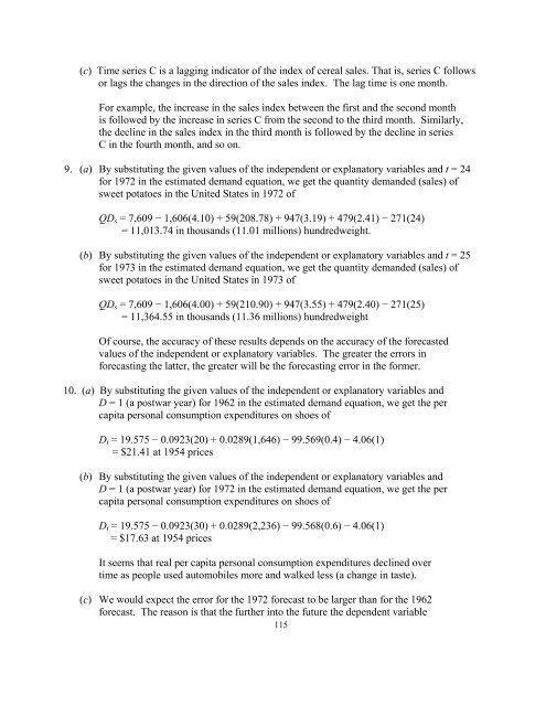
(c) Time series C is a lagging indicator of the index of cereal sales. That is, series C follows or lags the changes in the direction of the sales index. The lag time is one month. For example, the increase in the sales index between the first and the second month is followed by the increase in series C from the second to the third month. Similarly, the decline in the sales index in the third month is followed by the decline in series C in the fourth month, and so on. 9. (a) By substituting the given values of the independent or explanatory variables and t = 24 for 1972 in the estimated demand equation, we get the quantity demanded (sales) of sweet potatoes in the United States in 1972 of QD s = 7,609 − 1,606(4.10) + 59(208.78) + 947(3.19) + 479(2.41) − 271(24) = 11,013.74 in thousands (11.01 millions) hundredweight. (b) By substituting the given values of the independent or explanatory variables and t = 25 for 1973 in the estimated demand equation, we get the quantity demanded (sales) of sweet potatoes in the United States in 1973 of QD s = 7,609 − 1,606(4.00) + 59(210.90) + 947(3.55) + 479(2.40) − 271(25) = 11,364.55 in thousands (11.36 millions) hundredweight Of course, the accuracy of these results depends on the accuracy of the forecasted values of the independent or explanatory variables. The greater the errors in forecasting the latter, the greater will be the forecasting error in the former. 10. (a) By substituting the given values of the independent or explanatory variables and D = 1 (a postwar year) for 1962 in the estimated demand equation, we get the per capita personal consumption expenditures on shoes of D t = 19.575 − 0.0923(20) + 0.0289(1,646) − 99.569(0.4) − 4.06(1) = $21.41 at 1954 prices (b) By substituting the given values of the independent or explanatory variables and D = 1 (a postwar year) for 1972 in the estimated demand equation, we get the per capita personal consumption expenditures on shoes of D t = 19.575 − 0.0923(30) + 0.0289(2,236) − 99.568(0.6) − 4.06(1) = $17.63 at 1954 prices It seems that real per capita personal consumption expenditures declined over time as people used automobiles more and walked less (a change in taste). (c) We would expect the error for the 1972 forecast to be larger than for the 1962 forecast. The reason is that the further into the future the dependent variable 115
Page 1 and 2: ECON 3400H Managerial Economics Ins
Page 3: 6. (a) The exponential forecasts (F
Page 7 and 8: 14. (a) Wait for June 2012 when the
Page 9: ln Q 61 = 1.2789 − 0.1647(0.47) +

Suggested Solutions to Assignment 4 (Optional) - Trent University

You also want an ePaper? Increase the reach of your titles

Delete template?

Save as template?