Adaptivity with moving grids

Adaptivity with moving grids 87
We now consider two examples taken from Cao et al. (2002) of the application
of the GCL method, which allow direct comparison with the optimaltransport-based
methods described in Section 3.
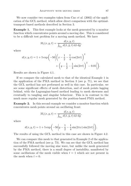
Example 1. This first example looks at the mesh generated by a monitor
function which concentrates points around a moving disc. This is considered
to be a difficult test problem for a moving mesh method. We have
M 1 (x, y, t) =
d(x, y, t)
∫Ω P
d(˜x, ỹ, t)d˜x dỹ ,
where
(
d(x, y, t) = 1 + 5 exp −50
∣
(x − 1 2 − 1 ) 2
4 cos(2πt)
(
+ y − 1 2 − 1 ) 2 )
4 sin(2πt) − 0.01
∣ .
Results are shown in Figure 4.1.
If we compare the calculated mesh to that of the identical Example 1 in
the application of the PMA method in Section 3 (see p. 71), we see that
the GCL method has not performed as well in this case. In particular, we
see some significant effects of mesh distortion, and of mesh points lagging
behind, with the Lagrangian-based method leading to mesh skewness and
eventually to tangling and singular behaviour. This is in contrast to the
much more regular mesh generated by the position-based PMA method.
Example 2. In this second example we consider a monitor function which
concentrates mesh points around an oscillating front:
M 1 (x, y, t) =
d(x, y, t)
∫Ω P
d(˜x, ỹ, t)d˜x dỹ ,
where
(
d(x, y, t) = 1 + 5 exp −50
∣ y − 1 2 − 1 ∣ ∣∣∣
).
4 sin(2πx)sin(2πt)
The results of using the GCL method in this case are shown in Figure 4.2.
We can compare this mesh to that generated in Example 2 of the application
of the PMA method (see p. 73). We can see that the GCL method has
successfully followed the moving sine wave, but unlike the mesh generated
by the PMA method, there is a small degree of instability, manifested by
some oscillations of the mesh visible when t = 1 which are not present in
the mesh when t =0.