Adaptivity with moving grids

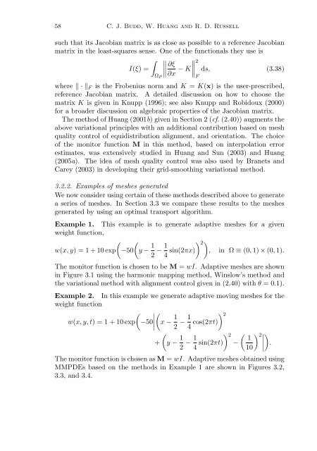
58 C. J. Budd, W. Huang and R. D. Russell
such that its Jacobian matrix is as close as possible to a reference Jacobian
matrix in the least-squares sense. One of the functionals they use is
∫ ∥ ∥ ∥∥∥ ∂ξ ∥∥∥
2
I(ξ) =
Ω P
∂x − K ds, (3.38)
F
where ‖·‖ F is the Frobenius norm and K = K(x) is the user-prescribed,
reference Jacobian matrix. A detailed discussion on how to choose the
matrix K is given in Knupp (1996); see also Knupp and Robidoux (2000)
for a broader discussion on algebraic properties of the Jacobian matrix.
The method of Huang (2001b) given in Section 2 (cf. (2.40)) augments the
above variational principles with an additional contribution based on mesh
quality control of equidistribution alignment, and orientation. The choice
of the monitor function M in this method, based on interpolation error
estimates, was extensively studied in Huang and Sun (2003) and Huang
(2005a). The idea of mesh quality control was also used by Branets and
Carey (2003) in developing their grid-smoothing variational method.
3.2.2. Examples of meshes generated
We now consider using certain of these methods described above to generate
a series of meshes. In Section 3.3 we compare these results to the meshes
generated by using an optimal transport algorithm.
Example 1. This example is to generate adaptive meshes for a given
weight function,
(
w(x, y) = 1 + 10 exp −50
(y − 1 2 − 1 ) 2 )
4 sin(2πx) , in Ω ≡ (0, 1) × (0, 1).
The monitor function is chosen to be M = wI. Adaptive meshes are shown
in Figure 3.1 using the harmonic mapping method, Winslow’s method and
the variational method with alignment control given in (2.40) with θ =0.1).
Example 2. In this example we generate adaptive moving meshes for the
weight function
(
w(x, y, t) = 1 + 10 exp −50
∣
(x − 1 2 − 1 ) 2
4 cos(2πt)
(
+ y − 1 2 − 1 ) 2 ( 1 2 ∣)
∣∣∣
4 sin(2πt) − .
10)
The monitor function is chosen as M = wI. Adaptive meshes obtained using
MMPDEs based on the methods in Example 1 are shown in Figures 3.2,
3.3, and 3.4.